Experimental construction of a W-superposition state and its equivalence to the GHZ state under local filtration

Abstract

We experimentally construct a novel three-qubit entangled W-superposition ($\rm W\bar{\rm W}$) state on an NMR quantum information processor. We give a measurement-based filtration protocol for the invertible local operation (ILO) that converts the $\rm W\bar{\rm W}$ state to the GHZ state, using a register of three ancilla qubits. Further we implement an experimental protocol to reconstruct full information about the three-party $\rm W\bar{\rm W}$ state using only two-party reduced density matrices. An intriguing fact unearthed recently is that the $\rm W\bar{\rm W}$ state which is equivalent to the GHZ state under ILO, is in fact reconstructible from its two-party reduced density matrices, unlike the GHZ state. We hence demonstrate that although the $\rm W\bar{\rm W}$ state is interconvertible with the GHZ state, it stores entanglement very differently.

I Introduction

Explorations of multiqubit entanglement have unearthed several families of states with curious quantum properties and there have been many attempts in recent years to characterize all the denizens of this quantum zoo Horodecki et al. (2009); Gühne and Töth (2009); Eltschka and Siewert (2014). The situation becomes complicated for systems of more than two qubits and correspondingly the classification of their entanglement turns out to be more involved de Vicente et al. (2012); Zhao et al. (2013).

Pure entangled states of three qubits fall into two categories, namely the GHZ- or the W-class, under stochastic local operations and classical communication (SLOCC) Acin et al. (2000); Kampermann et al. (2012) with the maximally entangled GHZ and W states being given by:

$$\left|{\rm GHZ}\right\rangle = \frac{1}{\sqrt{2}}\left(\left|{000}\right\rangle+\left|{111}\right\rangle\right)$$

$$|{\rm W}\rangle = \frac{1}{\sqrt{3}}\left(|001\rangle+|010\rangle+|100\rangle\right)$$ (1)

The entanglement of the GHZ state is fragile under qubit loss, i.e when any one of the qubits is traced out, the other two qubits become completely disentangled Chen and Chen (2006); Gühne and Töth (2009). Hence if one of the parties decides not to cooperate, the entanglement resources of the GHZ state cannot be used. In contradistinction to the GHZ state, the W-state residual bipartite entanglement is robust against qubit loss Gühne and Töth (2009).

It has been shown by Linden et. al., that almost every pure state of three qubits can be completely determined by its two-party reduced density matrices Linden et al. (2002). The two inequivalent entangled states, namely the W and GHZ states, have contrasting irreducibility features: while GHZ states have irreducible correlations and cannot be determined from their two-party marginals Walck and Lyons (2008, 2009), W-states are completely determined by their two-party marginals Diosi (2004); Cavalcanti et al. (2005); Parashar and Rana (2009). Tripartite entanglement has been studied experimentally using optics Roos et al. (2004); Mikami et al. (2005); Resch et al. (2005) and NMR Laflamme et al. (1998); Nelson et al. (2000); Teklemariam et al. (2002); Kawamura et al. (2006); Peng et al. (2010); Gao et al. (2013); Dogra et al. (2015).

Recently, the entanglement properties of a permutation symmetric superposition of the $\rm W$ state and its obverse $\bar{\rm W}=1/\sqrt{3}\left(|100\rangle+|101\rangle+|110\rangle\right)$ have been characterized Devi et al. (2012); Sudha et al. (2012):

$$|\rm W\bar{\rm W}\rangle=\frac{1}{\sqrt{2}}\left(\left|{\rm W}\right\rangle+\left|{\bar{\rm W}}\right\rangle\right)$$

$$=\frac{1}{\sqrt{6}}\left(|001\rangle+|010\rangle+|011\rangle+|100\rangle+|101\rangle+|110\rangle\right)$$

While this state (referred to henceforth as the $\rm W\bar{\rm W}$ state) belongs to the GHZ entanglement class, its correlation information (in contrast to the GHZ state) is uniquely contained in its two-party reduced states. The argument for reconstructing the three-qubit $\rm W\bar{\rm W}$ state from its two-party reduced states runs along similar lines to the original argument of Linden et. al. Linden et al. (2002). If we assume another state to have the same two-party reduced density matrices as the $\rm W\bar{\rm W}$ state, this constraint can be used to prove that the new state is no different from the original $\rm W\bar{\rm W}$ state Devi et al. (2012); Sudha et al. (2012).

In this work we focus on the $\rm W\bar{\rm W}$ state. We provide an explicit measurement-based filtration scheme to filter out the $\left|{\rm GHZ}\right\rangle$ state from the $\rm W\bar{\rm W}$ state. Further, we experimentally construct and tomograph the $\rm W\bar{\rm W}$ state on an NMR quantum information processor of three coupled qubits. We experimentally demonstrate that the information about tripartite correlations present in this state can indeed be completely captured by its two-party reduced density matrices. We reconstruct the experimental density matrices using complete state tomography and compare them with the theoretically expected states and also compute state fidelities. The GHZ class of states are an important computational resource Horodecki et al. (2009) and it has been shown that states that are SLOCC equivalent to these can be used for the same kind of quantum information processing tasks Gühne and Töth (2009). Therefore, it is expected that the $\rm W\bar{\rm W}$ state will also prove useful for quantum computation. Furthermore, the quantification of the tripartite correlation information present in this state is easier as compared to the GHZ state, as entanglement measurement requires only two-qubit detectors.

The paper is organized as follows: Section II describes how we obtain the ${\rm GHZ}$ state from the $\rm W\bar{\rm W}$ state by local filtration based on projective measurements using a register of three ancilla qubits. Section III describes the experimental creation of the $\rm W\bar{\rm W}$ superposition state on a three-qubit NMR quantum information processor. Section III.1 contains the details of the molecule used, the NMR pulse sequence for $\rm W\bar{\rm W}$ state construction and the results of state tomography. The information content of the $\rm W\bar{\rm W}$ as captured from its two-party marginals is described in Section III.2. We conclude in Section IV with some remarks about GHZ and W$\bar{\rm W}$ types of three-qubit entanglement and the relationship between entanglement class and how information about entanglement is stored in a quantum state.

II Filtration Protocol to show SLOCC equivalence of $\rm W\bar{\rm W}$ and GHZ

Measurement-based local filters have been used for entanglement manipulation in the context of violation of Bell inequalities as well as for the detection of bound entangled states Gisin (1996); Verstraete and Wolf (2002); Das et al. (2015). No local operations can convert a state from the GHZ class to the W class. However, surprisingly, it has been shown that the $\rm{W}\bar{\rm W}$ is in the GHZ class, deriving from the fact that it is related to the GHZ state via the SLOCC class of operations given by Devi et al. (2012); Sudha et al. (2012):

$$\left|{GHZ}\right\rangle\equiv A\otimes A\otimes A\left|{W\bar{W}}\right\rangle$$ (3)

with

$$A=\frac{1}{\sqrt{3}}\begin{pmatrix}1&\omega\\ 1&\omega^{2}\end{pmatrix}$$ (4)

being an ILO, where $\omega=e^{\iota\frac{2\pi}{3}}$ denotes the cube root of unity. We have used ‘$\equiv$’ instead of an equality sign in Eqn. (3) because $A$ is a non-unitary operator that does not preserve the norm and the two sides in Eqn. (3) do not have the same norm.

We now proceed to reinterpret $A$ as an action on an ensemble of identically prepared states $\rm W\bar{\rm W}$ and implement the operation described in Eqn. (3). In this process, we will have to discard some copies and the new ensemble that we construct with each member in the filtered GHZ state will have fewer copies as compared to the original ensemble of $\rm W\bar{\rm W}$ states. These aspects will be brought out more clearly when we describe the measurement-based filtration protocol to realize the ILO.

Since $A$ acts on each of the qubits locally, we first want to realize the operation $A$ on a single qubit. The non-unitary operator $A$ has a singular valued decomposition

$$A=UDV$$ (5)

where the unitary operators $U$ and $V$ are given by

$$U=\frac{e^{\iota\frac{\pi}{2}}}{\sqrt{2}}\begin{pmatrix}e^{-\iota\frac{\pi}{6}}&-e^{\iota\frac{\pi}{3}}\\ e^{\iota\frac{\pi}{6}}&-e^{-\iota\frac{\pi}{3}}\end{pmatrix},\quad V=\frac{1}{\sqrt{2}}\begin{pmatrix}-\iota&\iota\\ \iota&\iota\end{pmatrix}$$ (6)

and the non-unitary diagonal operator $D$ is given by

$$D=\begin{pmatrix}1&0\\ 0&\frac{1}{\sqrt{3}}\end{pmatrix}$$ (7)

The operators $U$ and $V$ are unitary and can be implemented via a local Hamiltonian evolution. Therefore, we now turn to the implementation of $D$ on a one-qubit state.

From the two columns of the operator $D$ we define two vectors

$$\left|{u_{1}}\right\rangle=\begin{pmatrix}1\\ 0\end{pmatrix}\quad{\rm and}\quad\left|{u_{2}}\right\rangle=\frac{1}{\sqrt{3}}\begin{pmatrix}0\\ 3^{\frac{1}{4}}\end{pmatrix}$$ (8)

These vectors are orthogonal to each other but are not normalized. We now extend the Hilbert space of the system by adding an ancilla qubit. We extend the vectors $u_{1}$ and $u_{2}$ to the composite Hilbert space formed by the ancilla and the system to obtain two four-dimensional vectors

$$\left|{\xi_{1}}\right\rangle=\begin{pmatrix}1\\ 0\\ 0\\ 0\end{pmatrix}\quad{\rm and}\quad\left|{\xi_{2}}\right\rangle=\frac{1}{\sqrt{3}}\begin{pmatrix}0\\ 3^{\frac{1}{4}}\\ 0\\ \sqrt{3-\sqrt{3}}\end{pmatrix}$$ (9)

The vectors $\left|{\xi_{1}}\right\rangle$ and $\left|{\xi_{2}}\right\rangle$ are not only mutually orthogonal but also normalized.

Using these orthonormal vectors $\left|{\xi_{1}}\right\rangle$ and $\left|{\xi_{2}}\right\rangle$, we construct orthogonal projectors $P_{1}$ and $P_{2}$

$$P_{1}=\left|{\xi_{1}}\right\rangle\left\langle{\xi_{1}}\right| = \begin{pmatrix}1&0&0&0\\ 0&0&0&0\\ 0&0&0&0\\ 0&0&0&0\end{pmatrix}$$

$$P_{2}=\left|{\xi_{2}}\right\rangle\left\langle{\xi_{2}}\right| = \frac{1}{\sqrt{3}}\begin{pmatrix}0&0&0&0\\ 0&1&0&\sqrt{\sqrt{3}-1}\\ 0&0&0&0\\ 0&\sqrt{\sqrt{3}-1}&0&\sqrt{3}-1\end{pmatrix}$$

We define the projection operator $P=P_{1}+P_{2}$. The effect of the projector $P$ on the composite system of the single qubit and a one-qubit ancilla turns out to be

$$P=\left(\begin{array}[]{c|c}D&\Delta\\ \hline\cr\Delta&D^{\prime}\end{array}\right)_{\displaystyle 4\times 4}$$ (11)

where $D$ is the diagonal part of the singular value decomposition of the operator $A$ given in Eqn. (7), the complementary matrix $D^{\prime}=I-D$ and the matrix $\Delta$ can be obtained readily from Eqn. (LABEL:projectors).

If we prepare the ancilla in a state $\left|{0}\right\rangle\left\langle{0}\right|$ with the system being in an arbitrary state $\rho$, the action of $P$ on the composite system is given by

$$P\left(\left|{0}\right\rangle\left\langle{0}\right|\otimes\rho\right)P=\left(\begin{array}[]{c|c}D\rho D&D\rho\Delta\\ \hline\cr\Delta\rho D&\Delta\rho\Delta\end{array}\right)$$ (14)

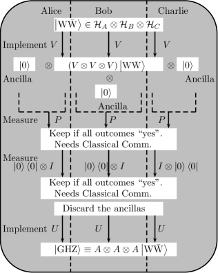
Figure 1: Schematic diagram of the filtration scheme to implement the non-unitary ILO transformation that converts a $\rm W\bar{\rm W}$ state to a GHZ state.

If we measure the projector $P$ on the composite system (system and ancilla), whenever the measurement gives a positive answer, the state after measurement is given by the right hand side of Eqn. (14). We retain only these cases and discard the state whenever the outcome of the measurement is negative. Further, on the final state given in Eqn. (14), we measure the projector $\left|{0}\right\rangle\left\langle{0}\right|$ on the ancilla alone. As before, if the outcome is positive we retain the state, and if the outcome is negative we discard the state. In case the outcome is positive, the resultant state is $\left|{0}\right\rangle\left\langle{0}\right|\otimes D\rho D$ and upon discarding the ancilla we get the state of the system to be $D\rho D$. This completes the application of the non-unitary invertible operator $D$ on $\rho$. Sandwiching this operation between the unitary transformations $U$ and $V$ as given in Eqn. (5), we achieve the application of the ILO operator $A$ on $\rho$.

The scheme is easily extendable to $2\otimes 2\otimes 2$ systems, where we locally implement $A$ on each of the three qubits. We imagine that the tripartite system is divided between Alice, Bob and Charlie and each of them can perform local operations at their location. We begin with the state $\left|{\rm W\bar{\rm W}}\right\rangle$ for the three qubits, attach a one-qubit ancilla to each qubit, and measure the local projector $P$ for each qubit. If the outcome of these measurements (that amount to a measurement of $P\otimes P\otimes P$) is positive we retain the state, otherwise we discard the state. Then on each ancilla, we measure the projector $\left|{0}\right\rangle\left\langle{0}\right|$ and retain the cases when all the outcomes are positive. Upon discarding the ancillas, the resultant state is the application of $D$ on each qubit. When we sandwich this process between the unitaries $U$ and $V$ on each qubit, we get the final state as $\left|{\rm GHZ}\right\rangle$. This process of measurement-based filtration is schematically explained in Fig. 1. To decide when to discard and when to retain the outcome, we require classical communication between Alice, Bob and Charlie. Since we discard the output state in a number of cases, the size of the ensemble obtained in the end is smaller than the original ensemble.

III NMR implementation

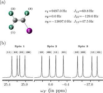
Figure 2: (a) Molecular structure and NMR parameters (chemical shifts and J-coupling in Hz) and ¹⁹F NMR spectrum of trifluoroiodoethylene. The three fluorine spins correspond to the three-qubit system. (b) The 1D ¹⁹F NMR thermal equilibrium spectrum obtained after a $\frac{\pi}{2}$ readout pulse. The NMR transitions of each qubit are labeled by the corresponding logical states of the other two qubits.

To prepare the $\rm W\bar{\rm W}$ state on a three-qubit NMR quantum information processor, we employ the three fluorine (spin-1/2) qubits of trifluoroiodoethylene. The molecular structure and NMR parameters of this three-qubit system are adequate for the kind of manipulations involved in quantum state preparation and are given in Fig. 2(a). Average fluorine longitudinal T₁ relaxation times of 5.0 s and T₂ relaxation times of 1.0 s were experimentally determined. The equilibrium fluorine NMR spectrum obtained after a $\frac{\pi}{2}$ readout pulse is shown in Fig. 2(b).

The system was first initialized into the $|000\rangle$ pseudopure state using the standard spatial averaging technique Cory et al. (1998). The experimental density matrices were tomographed by standard state tomography procedures Chuang et al. (1998); Long et al. (2001); Leskowitz and Mueller (2004). The three-qubit experimental density matrix was tomographed using a set of eleven detection operators defined by {III, IIX, IXI, XII, IIY, IYI, YII, YYI, IXX, XXX, YYY}, and the two, two-qubit reduced density matrices were determined using a set of four detection operators defined by {III, IXI, IYI, XXI} and {III, IIX, IIY, IXX} respectively, with I denoting the identity (or no-operation) operator and X(Y) denoting a spin-selective $\frac{\pi}{2}$ pulse of X(Y) phase on a specified qubit. The fidelity of the reconstructed state was computed using the Uhlmann-Jozsa fidelity measure Uhlmann (1976); Jozsa (1994):

$$F=\left(Tr\left(\sqrt{\sqrt{\rho_{\rm theory}}\rho_{\rm expt}\sqrt{\rho_{\rm theory}}}\right)\right)^{2}$$ (15)

where $\rho_{\rm theory}$ and $\rho_{\rm expt}$ denote the theoretical and experimental density matrices respectively.

III.1 $\rm W\bar{\rm W}$ construction scheme

The circuit to construct a $\rm W\bar{\rm W}$ state consists of several single-qubit and two-qubit gates. A single-qubit gate $\rm U_{i}[\alpha]_{y}$ acting on the $i$th qubit, achieves a rotation by the angle $\alpha$ around the $y$ axis with a corresponding unitary matrix given by:

$$U_{i}[\alpha]_{y}=\left(\begin{array}[]{cc}\cos{\frac{\alpha}{2}}&-\sin{\frac{\alpha}{2}}\\ \sin{\frac{\alpha}{2}}&\cos{\frac{\alpha}{2}}\end{array}\right)$$ (16)

A two-qubit controlled-rotation gate CR${}_{ij}[\phi]_{y}$, implements the single-qubit rotation $U_{j}[\phi]_{y}$ on the target qubit $j$ about the $y$ axis, if the control qubit $i$ is in the state $|1\rangle$. The $\rm CNOT_{ij}$ gate implements a controlled-NOT operation with the $i$th qubit as control and the $j$th qubit as target.

The sequence of gates to construct a $\rm W\bar{\rm W}$ state, starting from the initial pseudopure state $|000\rangle$ is given as:

$$|000\rangle$$

$$\downarrow\framebox[35.56593pt]{ $\scriptstyle U_{1}\left[-\frac{\pi}{3}\right]_{y}$ }\downarrow$$

$$\frac{1}{2}\left(\sqrt{3}|000\rangle-|100\rangle\right)$$

$$\downarrow\framebox[85.35826pt]{ $\scriptstyle{\rm CR}_{12}\left[2\cos^{-1}{(1/\sqrt{3})}\right]_{y}$}\downarrow$$

$$\frac{1}{2}\left(\sqrt{3}|000\rangle-\frac{1}{\sqrt{3}}|100\rangle-\sqrt{\frac{2}{3}}|110\rangle\right)$$

$$\downarrow{\framebox[42.67912pt]{$\scriptstyle{\rm CR}_{21}\left[-\frac{\pi}{2}\right]_{y}$}}\downarrow$$

$$\frac{1}{2}\left(\sqrt{3}|000\rangle-\frac{1}{\sqrt{3}}\left(|100\rangle+|110\rangle+|010\rangle\right)\right)$$

$$\downarrow{\framebox[42.67912pt]{$\scriptstyle{\rm CNOT}_{13}$}}\downarrow$$

$$\frac{1}{2}\left(\sqrt{3}|000\rangle-\frac{1}{\sqrt{3}}\left(|101\rangle+|111\rangle+|010\rangle\right)\right)$$

$$\downarrow{\framebox[42.67912pt]{$\scriptstyle{\rm CNOT}_{23}$}}\downarrow$$

$$\frac{1}{2}\left(\sqrt{3}|000\rangle-\frac{1}{\sqrt{3}}\left(|101\rangle+|110\rangle+|011\rangle\right)\right)$$

$$\downarrow{\framebox[85.35826pt]{$\scriptstyle\rm U_{1}\left[\frac{\pi}{2}\right]_{y}\rm U_{2}\left[\frac{\pi}{2}\right]_{y}\rm U_{3}\left[\frac{\pi}{2}\right]_{y}$}}\downarrow$$

$$\frac{1}{\sqrt{6}}\left(|001\rangle+|010\rangle+|011\rangle+|100\rangle+|101\rangle+|110\rangle\right)$$

The quantum circuit to construct the $\rm W\bar{\rm W}$ state on a three-qubit system is given in Fig. 3(a).

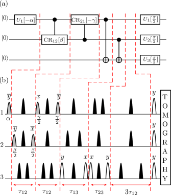
Figure 3: (a) Quantum circuit showing sequence of gates required to construct the $\rm W\bar{\rm W}$ state, starting from the pseudopure state $|000\rangle$. The gate operations are described in the main text and all the rotations take place about the $y$-axis. (b) NMR pulse sequence to create a $\rm W\bar{\rm W}$ state. All the pulses are low-power selective pulses represented by shaped blocks. Filled black shapes are $\pi$ refocusing pulses, unfilled shapes correspond to pulses of $\frac{\pi}{2}$ flip angle and the gray shaded shapes are labeled with their specific flip angles and phases. The axes of rotation are specified at the top of each pulse. Vertical dotted red lines show the correspondence between the quantum circuit and the experimental pulse sequence. All pulses are of phase $x$ unless otherwise labeled. The values of the rf pulse flip angles used are $\alpha=\frac{\pi}{3},\beta=2\cos^{-1}{(\frac{1}{\sqrt{3}})},\gamma=\frac{\pi}{2}$ and $\tau_{ij}$ represents an evolution under the $J_{ij}$ coupling. The last $3\tau_{12}$ period is used to compensate the extra phase acquired (as described in the text).

The NMR pulse sequence to create the $\rm W\bar{\rm W}$ state, starting from the pseudopure state $|000\rangle$ is given in Fig. 3(b). All the pulses are shaped pulses, labeled by the corresponding axes of rotation and the flip angles; $\tau_{ij}$ denotes an evolution period under the $J_{ij}$ coupling. Refocusing ($\pi$) pulses are applied in the middle of the evolution periods to compensate for chemical shift evolution and pairs of $\pi$ pulses are introduced at $1/4$ and $3/4$ of the evolution periods to eliminate undesired J-evolutions. After the evolution interval $\tau_{23}$ and the $[\frac{\pi}{2}]_{y}$ on the third qubit (corresponding to a $\rm CNOT_{23}$ gate), the state obtained is $\frac{\sqrt{3}}{2}|000\rangle-\frac{1}{2\sqrt{3}}(\iota|101\rangle+|110\rangle+\iota|011\rangle)$. There is an undesirable extra relative phase of ‘$\iota$’ that has accumulated between two of the basis vectors. This undesired extra phase factor is compensated for during the evolution interval $3\tau_{12}$. The implementation of the last module (simultaneous $[\frac{\pi}{2}]_{y}$ pulses on all the three qubits) results in the desired $\rm W\bar{\rm W}$ state with no extra relative phase. All the selective pulses are $265~{}\mu$s “Gauss” shaped pulses and the non-selective excitation pulse is a frequency-modulated $400~{}\mu$s “Gauss” shaped pulse.

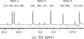
Figure 4: The 1D ¹⁹F NMR spectrum corresponding to the creation of the $\rm W\bar{\rm W}$ state. The NMR transitions of each qubit are labeled by the corresponding logical states of the other two qubits.

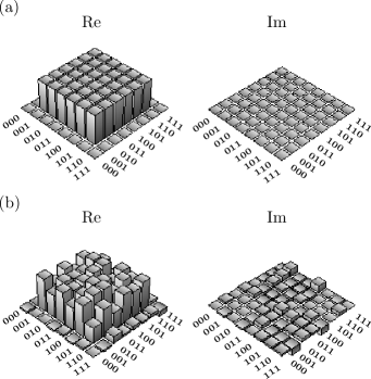
Figure 5: The real (Re) and imaginary (Im) parts of the (a) theoretically expected and (b) experimentally density matrices for the $\rm W\bar{\rm W}$ state reconstructed using full state tomography. The rows and columns of the bar graphs depict the computational basis of the three qubits in binary order from $|000\rangle$ to $|111\rangle$. The experimentally tomographed state has a fidelity of 0.94.

The NMR spectrum of the $\rm W\bar{\rm W}$ state obtained by a sequence of selective rotations on the initial pseudopure state is shown in Fig. 4. Each spin multiplet has two resonance peaks (as compared to four resonance peaks for the thermal equilibrium state). The expected NMR spectral pattern of an ideal $\rm W\bar{\rm W}$ state should contain resonance peaks of equal magnitude and phase, and deviations from ideal spectral peak intensities and phases in the experimentally obtained spectrum, can be attributed to imperfections in the rf pulse calibrations and to relaxation during the selective pulse durations.

The tomograph of the experimentally constructed $\rm W\bar{\rm W}$ state is shown in Fig. 5. The experimentally tomographed state was compared with the theoretically expected state and the density matrices match well, within experimental error, with a computed state fidelity of 0.94 (the fidelity was computed from Eqn. 15).

III.2 Reconstruction of $\rm W\bar{\rm W}$ from two-party reduced density matrices

A protocol was developed Diosi (2004) to validate the surprising aspect of multi-party correlations asserted by Linden et. al. Linden et al. (2002); Linden and Wootters (2002), that the information about three-party correlations of almost all pure three-qubit states (except for GHZ-type states) are already contained in their corresponding two-party reduced states. We delineate below the argument for how a general three-qubit pure state $\rho_{ABC}$ can be completely determined by using any of the equivalent sets $(\rho_{AB},\rho_{AC})$, $(\rho_{AB},\rho_{BC})$, or $(\rho_{AC},\rho_{BC})$ of reduced two-party states. The reduced single-qubit reduced state $\rho_{A}$ and the two-qubit reduced state $\rho_{BC}$ share the same set of eigen values, and can hence be written as Diosi (2004):

$$\rho_{A} = \sum_{i}p_{A}^{i}\left|{i}\right\rangle\left\langle{i}\right|$$

$$\rho_{BC} = \sum_{i}p_{A}^{i}\left|{i;BC}\right\rangle\left\langle{i;BC}\right|$$ (17)

where $\{\left|{i}\right\rangle\}$ are the eigenvectors of $\rho_{A}$ with eigenvalues $\{p_{A}^{i}\}$, and $\{\left|{i;BC}\right\rangle\}$ are the eigenvectors of $\rho_{BC}$ with eigenvalues $\{p_{A}^{i}\}$. Furthermore, the three-qubit pure states that are compatible with $\rho_{A}$ and $\rho_{BC}$ are given by:

$$\left|{\psi_{ABC};\alpha}\right\rangle=\sum_{i}e^{\iota\alpha_{i}}\sqrt{p_{A}^{i}}\left|{i}\right\rangle\otimes\left|{i;BC}\right\rangle$$ (18)

Similarly, the three-qubit pure states that are compatible with $\rho_{C}$ and $\rho_{AB}$ are given by

$$\left|{\psi_{ABC};\gamma}\right\rangle=\sum_{k}e^{\iota\gamma_{k}}\sqrt{p_{c}^{k}}\left|{k;AB}\right\rangle\otimes\left|{k}\right\rangle$$ (19)

where $\{\left|{k}\right\rangle\}$ are the eigenvectors of $\rho_{C}$ with eigenvalues $\{p_{c}^{k}\}$ and $\{\left|{k;AB}\right\rangle\}$ are the corresponding eigenvectors of $\rho_{AB}$. Since the pure state $\left|{\psi_{ABC}}\right\rangle$ is compatible with both $\rho_{AB}$ and $\rho_{BC}$, we can now consistently find the values of $\alpha_{i}$ and $\gamma_{k}$ while ensuring that $\left|{\psi_{ABC};\alpha}\right\rangle=\left|{\psi_{ABC};\gamma}\right\rangle$.

We used the set of two, two-party reduced states $(\rho_{AB},\rho_{BC})$, to reconstruct the full three-qubit $\rm W\bar{\rm W}$ state. The reconstructed density matrix for the $\rm W\bar{\rm W}$ state, using two sets of the corresponding two-qubit reduced density matrices ($\rho_{AB},\rho_{BC}$) is given in Fig. 6. The two-party reduced states were able to reconstruct the three-party $\rm W\bar{\rm W}$ state with a fidelity of 0.92, which matches well with the full reconstruction of the entire three-qubit state given in Fig. 5(b).

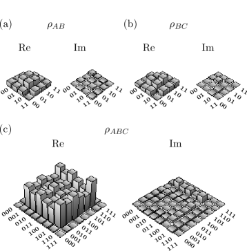
Figure 6: The real (Re) and imaginary (Im) parts of the tomographed density matrix for the state $\rm W\bar{\rm W}$ state. (a) The two-qubit reduced density matrix $\rho_{AB}$. (b) The two-qubit reduced density matrix $\rho_{BC}$. (c) The entire three-qubit density matrix $\rho_{ABC}$, reconstructed from the corresponding two-qubit reduced density matrices. The rows and columns in the bar graphs encode the computational basis of the qubits, from $|00\rangle$ to $|11\rangle$ for two qubits and from $|000\rangle$ to $|111\rangle$ for three qubits. The fidelity between the three-qubit state ($\rho_{ABC}$) reconstructed from the two-qubit density matrices and the three-qubit state obtained by complete three-qubit state tomography is found to be 0.92.

IV Conclusions

We described a measurement-based filtration scheme to demonstrate the ILO equivalence of the $\rm W\bar{\rm W}$ state with the $\rm GHZ$ state. We experimentally implemented an NMR-based scheme to construct a $\rm W\bar{\rm W}$ state. We were able to show that the three-qubit density operator $\rho_{ABC}$ obtained by full state tomography matches well with the same three-qubit state reconstructed using a set of two-party reduced density operators $(\rho_{AB},\rho_{BC})$. Thus, although the $\rm W\bar{\rm W}$ state belongs to the same entanglement class as the GHZ state, the two states store information about multi-party correlations in completely different ways. We thus experimentally demonstrated an interesting feature of multi-qubit entanglement namely, that two different entangled states belonging to the same SLOCC class can yet have their correlations exhibiting contrasting irreducible properties.

Since distinguishing entangled states is still a hard task, our work can be used as a benchmark to further classify how different entangled states store information about their correlations. Our work also has important implications for comparing the utility of different kinds of entangled states to perform the same computational task. We were unable to find a suitable molecular architecture to experimentally implement the ILO, since this requires each of the three qubits to be coupled to a separate one-qubit ancilla. However, it is a worthwhile exercise to look for an experimental implementation of the filtering protocol to perform the ILO. A further issue with such an implementation is the involvement of projective measurements, which are not straightforward to achieve using NMR.