Distinguishing Cause from Effect Based on Exogeneity

Abstract

Recent developments in structural equation modeling have produced several methods that can usually distinguish cause from effect in the two-variable case. For that purpose, however, one has to impose substantial structural constraints or smoothness assumptions on the functional causal models. In this paper, we consider the problem of determining the causal direction from a related but different point of view, and propose a new framework for causal direction determination. We show that it is possible to perform causal inference based on the condition that the cause is “exogenous" for the parameters involved in the generating process from the cause to the effect. In this way, we avoid the structural constraints required by the SEM-based approaches. In particular, we exploit nonparametric methods to estimate marginal and conditional distributions, and propose a bootstrap-based approach to test for the exogeneity condition; the testing results indicate the causal direction between two variables. The proposed method is validated on both synthetic and real data.

1 Introduction

Understanding causal relations allows us to predict the effect of changes in a system and control the behavior of the system. Since randomized experiments are usually expensive and often impracticable, causal discovery from non-experimental data has attracted much interest [18, 23]. To do this, it is crucial to find (statistical) properties in the non-experimental data that give clues about causal relations. For instance, under the causal Markov condition and faithfulness assumption, the causal structure can be partially estimated by constraint-based methods, which make use of conditional independence relationships.

Here we are concerned with the two-variable case, in which constraint-based methods, such as the PC algorithm [23], do not apply. We assume that the given observations are i.i.d., i.e., there is no temporal information. Recently, causal discovery based on structural equation models (SEMs) has proved useful in distinguishing cause from effect [21, 8, 27, 26, 15, 29]; however, the performance of such approaches depends on assumptions on the functional model class and/or on the data-generating functions. On the other hand, there have been attempts in different fields to characterize properties related to causal systems. One such concept (or family of concepts) is known as exogeneity, which is salient in econometrics [3, 4]. Roughly speaking, the notion expresses the property that the process that determines one variable $X$ is in some sense separate from or independent of the process that determines another variable, say $Y$, given the value of $X$.

The sense of “separateness" or “independence" in the rough idea has been specified in several ways for different purposes, which result in different concepts of exogeneity. The concept that is most relevant in this paper is the one in the context of model reduction, which was originally proposed as a condition that justifies inferences about the parameters of interest based on the conditional likelihood function rather than the joint likelihood function [7]. Here is the basic idea. Suppose the joint distribution of $(X,Y)$ can be factorized as

$$p(X,Y|\theta,\psi)=p(Y|X,\psi)p(X|\theta).$$ (1)

where the conditional distribution $p(Y|X)$ is parameterized by $\psi$ alone, and the marginal distribution $p(X)$ by $\theta$ alone. According to [3, 19], $X$ is said to be exogenous for $\psi$ (or any parameter of interest that is a function of $\psi$), if $\psi$ and $\theta$ are variation free, or in other words, are not subject to ‘cross-restrictions". From the frequentist point of view, this implies that $\psi$ and $\theta$ are independently estimable: the MLE of $\psi$ and that of $\theta$ are statistically independent according to the sampling distribution. From the Bayesian point of view [4], this implies that $\psi$ and $\theta$ are a posteriori independent given independent priors on them.

In this paper we will exploit the above idea to develop a test of whether there exists a parameterization $(\theta,\psi)$ for $p(X,Y)$ such that $X$ is exogenous for $\psi$, the parameters for $p(Y|X)$. The test is based on bootstrap and is applicable in nonparametric settings. We will also argue that if $X$ is a cause of $Y$ and there is no confounding, then there should exist a parameterization such that $X$ is exogenous for the parameters for $p(Y|X)$. Thus the nonparametric test can be used to indicate the causal direction between two variables, when the test passes for one direction but fails for the other. Compared to the SEM-based approach, an important novelty of this work is to use exogeneity as a new criterion for causal discovery in general settings, which allows distinguishing cause from effect and detecting confounders without structural constraints on the causal mechanism.

2 Exogeneity and causality

In this section we define what “exogeneity" means in this paper, and explain its link to causal asymmetry. The concept of exogeneity we will use is adapted from the concept known in econometrics as weak exogeneity, which is in itself a statistical rather than a causal concept. We will show that this statistical notion can nonetheless be exploited to formulate a method that can often determine the causal direction between two variables.

2.1 Exogeneity

The concept of weak exogeneity, as formulated by Engle, Hendry, and Richard (EHR) [3], is concerned with when efficient estimation of a set of parameters of interest can be made in a conditional submodel. For the purpose of this paper, suppose we are given two continuous random variables $X$ and $Y$, on which we have i.i.d. observations that are drawn according to a joint density $p(X,Y|\phi)$. By a reparameterization we mean a one-to-one transformation of the parameter set $\phi$. Our definition below is adapted from the EHR definition, adjusted for our present purpose and setup:

Definition 1 (Exogeneity of $X$ for $p(Y|X)$)

Suppose $p(X,Y)$ is parameterized by $\phi$. $X$ is said to be exogenous for the conditional $P(Y|X)$ (or simply, exogenous relative to $Y$) if and only if there exists a reparameterization $\phi\rightarrow(\theta,\psi)$, such that
(i.) $p(X,Y|\theta,\psi)=p(Y|X,\psi)p(X|\theta)$, and
(ii.) $\theta$ and $\psi$ are variation free, i.e., $(\theta,\psi)\in\Theta\times\Psi$, where $\Theta$ and $\Psi$ denote the set of admissible values of $\theta$ and $\psi$, respectively.

Here “variation free" means that the possible values that one parameter set can take do not depend on the values of the other set. Clauses (i.) and (ii.) in Definition 1 are the defining conditions for the concept of a (classical) cut: $[(Y|X;\psi),(X;\theta)]$ is said to operate a (classical) cut on $p(X,Y|\theta,\psi)$ if (i.) and (ii.) are satisfied. The cut implies that the maximum likelihood estimates of $\theta$ and $\psi$ can be computed from $p(X|\theta)$ and $p(Y|X,\psi)$, respectively, and so the MLEs $\hat{\theta}$ and $\hat{\psi}$ are independent according to the sampling distribution. The concept of exogeneity formalizes the idea that the mechanism generating the exogenous variable $X$ does not contain any relevant information about the parameter set $\psi$ for the conditional model $p(Y|X)$.

The concept of cut also has a Bayesian version: [4, 16].

Definition 2 (Bayesian cut)

$[(Y|X;\psi),(X;\theta)]$ operates a Bayesian cut on $p(X,Y|\theta,\psi)$ if
(i.) $\psi$ and $\theta$ are independent a priori, i.e., $\psi\mathchoice{\mathrel{\hbox to0.0pt{$\displaystyle\perp$\hss}\mkern 2.0mu{\displaystyle\perp}}}{\mathrel{\hbox to0.0pt{$\textstyle\perp$\hss}\mkern 2.0mu{\textstyle\perp}}}{\mathrel{\hbox to0.0pt{$\scriptstyle\perp$\hss}\mkern 2.0mu{\scriptstyle\perp}}}{\mathrel{\hbox to0.0pt{$\scriptscriptstyle\perp$\hss}\mkern 2.0mu{\scriptscriptstyle\perp}}}\theta$,
(ii.) $\theta$ is sufficient for the marginal process of generating $X$, i.e., $\psi\mathchoice{\mathrel{\hbox to0.0pt{$\displaystyle\perp$\hss}\mkern 2.0mu{\displaystyle\perp}}}{\mathrel{\hbox to0.0pt{$\textstyle\perp$\hss}\mkern 2.0mu{\textstyle\perp}}}{\mathrel{\hbox to0.0pt{$\scriptstyle\perp$\hss}\mkern 2.0mu{\scriptstyle\perp}}}{\mathrel{\hbox to0.0pt{$\scriptscriptstyle\perp$\hss}\mkern 2.0mu{\scriptscriptstyle\perp}}}X|\theta$, and
(iii.) $\psi$ is sufficient for the conditional process of generating $Y$ given $X$, i.e., $\theta\mathchoice{\mathrel{\hbox to0.0pt{$\displaystyle\perp$\hss}\mkern 2.0mu{\displaystyle\perp}}}{\mathrel{\hbox to0.0pt{$\textstyle\perp$\hss}\mkern 2.0mu{\textstyle\perp}}}{\mathrel{\hbox to0.0pt{$\scriptstyle\perp$\hss}\mkern 2.0mu{\scriptstyle\perp}}}{\mathrel{\hbox to0.0pt{$\scriptscriptstyle\perp$\hss}\mkern 2.0mu{\scriptscriptstyle\perp}}}Y|(\psi,X)$.

A Bayesian cut allows a complete separation of inference (on $\theta$) in the marginal model and of inference (on $\psi$) in the conditional model. The prior independence between $\theta$ and $\psi$ in the Bayesian cut is a counterpart to the variation-free condition in the classical cut, and the last two conditions in Definition 2 implies condition (i.) in Definition 1. Thus, the Bayesian cut is equivalent to the classical cut in sampling theory, and for the purpose of this paper can be regarded as interchangeable. Therefore, the exogeneity of $X$ relative to $Y$ can also be defined as that there exists a reparameterization $(\theta,\psi)$ of $p(X,Y)$ such that $[(Y|X;\psi),(X;\theta)]$ operates a Bayesian cut on $p(X,Y|\theta,\psi)$.

2.2 Possible Situations Where the Parameterization Fails to Operate a Bayesian Cut

Fig. 1(a) shows a data-generating process of $X$ and $Y$ from where $[(Y|X;\psi),(X;\theta)]$ operates a Bayesian cut. Note that in Definition 2, the two requirements of sufficiency of $\psi$ and $\theta$ for the marginal and the conditional (conditions (ii.) and (iii.)), respectively, are only restrictive under the assumption of prior independence of $\theta$ and $\psi$ (condition (i.)); otherwise, conditions (ii.) and (iii.) can be trivially met by, for example, taking $\theta$ and $\psi$ to be the same. In fact, any two conditions in Definition 2 could be trivial, given that the other does not hold. Fig. 1(b–d) shows the situations where conditions (i.), (ii.), and (iii.) are violated, respectively. In all those situations, $\theta$ and $\psi$ are not independent a posteriori.

(a)                           (b)

(c)                           (d)

Figure 1: Graphical representation of the data-generating process. (a) $[(Y|X;\psi),(X;\theta)]$ operates a Bayesian cut (implying that $X$ and $\psi$ are mutually exogenous). (b), (c), and (d) correspond to three situations where $[(Y|X;\psi),(X;\theta)]$ does not operate a Bayesian cut: (b) $\psi$ and $\theta$ are dependent a priori, as both of them depend on $\gamma$, which is a function of $\theta$ or $\psi$; (c) $\theta$ is not sufficient in modeling the marginal distribution of $X$, where $\gamma$ is a function of $\psi$; (d) $\psi$ is not sufficient in modeling the conditional distribution of $Y$ given $X$, where $\gamma$ is a function of $\theta$.

2.3 Relation to Causality

As Pearl [18] rightly stressed, the EHR concept of weak exogeneity is a statistical rather than a causal notion. Unlike the concept of super exogeneity, it is not defined in terms of interventions or multiple regimes. That is why, as we will show, the hypothesis that $X$ is exogenous relative to $Y$ in the sense we defined is generally testable by observational data. However, it is also linked to causality in that it is arguably a necessary condition for an unconfounded causal relation: if $X$ is a cause of $Y$ and there is no common cause of $X$ and $Y$, then $X$ is exogenous relative to $Y$ in the sense we defined. This follows from the principle we indicated at the beginning: if $X$ is an unconfounded cause of $Y$, then the process or mechanism that determines $X$ is separate or independent from the process or mechanism that determines $Y$ given $X$. The separation of processes ensures the existence of separate parameterizations of the processes, which will then satisfy our definition of exogeneity.

We have argued that if $X$ and $Y$ are causally related and unconfounded, the exogeneity property holds for the correct causal direction. Furthermore, if it turns out that there is one and only one direction that admits exogeneity, then the direction for which the exogeneity property holds must be the correct causal direction. This suggests the following approach to inferring the causal direction between $X$ and $Y$ based on some tests of exogeneity, assuming that $X$ and $Y$ are causally related and that there is no common cause of $X$ and $Y$ (or in other words, $X$ and $Y$ form a causally sufficient system): test whether (1) $X$ is exogenous for $p(Y|X)$ and whether (2) $Y$ is exogenous for $p(X|Y)$, and if one of them holds and the other does not, we can infer the causal direction accordingly. Of course it may also turn out that neither (1) nor (2) holds, which will indicate that the assumption of causal sufficiency is not appropriate, or that both (1) and (2) hold, which will indicate that the causal direction in question is not identifiable by our criterion.

A familiar example of a non-identifiable situation is when $X$ and $Y$ follow a bivariate normal distribution. In that case, as shown by EHR [3], there is a cut $[(Y|X;\psi),(X;\theta)]$ in one direction, as well as a cut $[(X|Y;\tilde{\psi}),(Y;\tilde{\theta})]$ in the other. Below we give an example where the causal direction is identifiable based on exogeneity.

An example of identifiable situation: Linear non-Gaussian case.

Let $X$ follow a Gaussian mixture model with two Gaussians, $X\sim\sum_{i=1}^{2}\pi_{i}\mathcal{N}(u_{i},\sigma_{i}^{2})$, where $\pi_{i}>0$ and $\pi_{1}+\pi_{2}=1$, and let $Y=c+\beta X+E$ where $E\sim\mathcal{N}(0,\sigma^{2})$. Therefore $\theta=\{\pi_{i},\mu_{i},\sigma_{i}\}_{i=1}^{2}$ and $\psi=\{c,\beta,\sigma^{2}\}$. We then have

$$p(X,Y|\theta,\beta) =\sum_{i}\pi_{i}\mathcal{N}(x;\mu_{i},\sigma_{i}^{2})\mathcal{N}(y;c+\beta x,\sigma^{2})$$

$$=\sum_{i}\pi_{i}\mathcal{N}(y;\tilde{\mu}_{i},\tilde{\sigma}_{i}^{2})\mathcal{N}(x;\tilde{c}_{i}+\tilde{\beta}_{i}y,\gamma_{i}^{2}),$$

where $\tilde{\mu}_{i}=c+\beta\mu_{i}$, $\tilde{\sigma}_{i}^{2}=\beta^{2}\sigma_{i}^{2}+\sigma^{2}$, $\tilde{c}_{i}=\frac{\mu_{i}\sigma^{2}-c\beta\sigma_{i}^{2}}{\beta\sigma_{i}^{2}+\sigma^{2}}$, $\tilde{\beta}_{i}=\frac{\beta\sigma_{i}^{2}}{\beta\sigma_{i}^{2}+\sigma^{2}}$, and $\gamma_{i}^{2}=\frac{\sigma^{2}\sigma_{i}^{2}}{\beta\sigma_{i}^{2}+\sigma^{2}}$. That is,

$$Y \sim\sum_{i=1}^{2}\pi_{i}\mathcal{N}(y;\tilde{u}_{i},\tilde{\sigma}_{i}^{2}),\textrm{~{}~{}and~{}~{}}$$

$$p(X|Y,\theta,\psi) =\sum_{i}\frac{\pi_{i}\mathcal{N}(y;\tilde{\mu}_{i},\tilde{\sigma}_{i}^{2})}{p(Y|\theta,\psi)}\cdot\mathcal{N}(x;\tilde{c}_{i}+\tilde{\beta}_{i}y,\gamma_{i}^{2}).$$

Clearly, if $\pi_{1}\pi_{2}\neq 0$, no matter how one parametrizes the density of $Y$, the conditional distribution of $X$ given $Y$ would involves those parameters that model the marginal density of $Y$. The sufficient parameter set of the distribution of $Y$, $\tilde{\theta}$, and that of the conditional distribution of $X$ given $Y$, $\tilde{\psi}$, cannot be variation-free or independent a priori; see Fig. 1(b). Alternatively, one can keep those parameters that are independent a priori from $\tilde{\theta}$ in $\tilde{\psi}$, i.e., $\tilde{\psi}$ and $\tilde{\theta}$ become independent a priori, but $\tilde{\psi}$ is then not sufficient in modeling $p(X|Y)$; see Fig. 1(d). In both situations $Y$ is not exogenous for $\tilde{\psi}$. Hence in this linear non-Gaussian case the exogeneity condition only holds for the direction $X\rightarrow Y$, and the causal direction is identifiable. Fig. 2 gives an intuitive illustration on how the shape of $P(Y)$ and that of $E(X|Y)$, which is determined by $P(X|Y)$, are related.

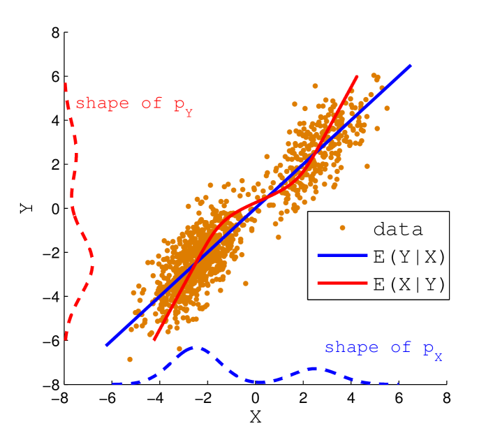
Figure 2: An illutration on the identifiability of a linear non-Gaussian model based on “exogeneity". $X$ is generated by a mixture of two Gaussians, and $Y$ is generated by $Y=X+E$, where $E\sim\mathcal{N}(0,1)$. Here $X$ is exogenous for parameters in $p_{Y|X}$, while $Y$ is not exogenous for parameters in $p_{X|Y}$.

3 Causal direction determination by testing for exogeneity with bootstrap

We now describe our approach to testing exogeneity. We will first illustrate how bootstrap can be used to test whether a given parametric model constitutes a (Bayesian) cut, and then develop a nonparametric test for exogeneity based on bootstrap.

3.1 Bootstrap-Based Test for Bayesian Cut in the Parametric Case

In this section, we assume that a parametric form $p(X,Y|\theta,\psi)=p(X|\theta)p(Y|X,\psi)$ is given. We would like to see whether the estimates of $\theta$ and of $\psi$ in (1) are independent, according to the sampling distribution; in other words, with a noninformative prior, we want to test if the posterior distribution $p(\theta,\psi|\mathcal{D})$ has no coupling between $\theta$ and $\psi$. In this case we are examining if $[(Y|X;\psi),(X;\theta)]$ operates a Bayesian cut.

Table 1: Notation involved in the proposed method based on exogeneity and bootstrap

$(\mathbf{x},\mathbf{y})$	given sample of $(X,Y)$
$(\mathbf{x}^{*(b)},\mathbf{y}^{*(b)})$	$b$th bootstrap resample
$\hat{\theta}^{*(b)},\hat{\psi}^{*(b)}$	estimate of parameters $\theta$ and $\psi$ on $(\mathbf{x}^{*(b)},\mathbf{y}^{*(b)})$
$\hat{p}^{*(b)}(X=\tilde{\mathbf{x}})$	marginal densities estimated on $(\mathbf{x}^{*(b)},\mathbf{y}^{*(b)})$ evaluated at $X=\tilde{\mathbf{x}}$
$\hat{p}^{*(b)}(Y|X=\tilde{\mathbf{x}})$	conditional densities estimated on $(\mathbf{x}^{*(b)},\mathbf{y}^{*(b)})$ evaluated at $X=\tilde{\mathbf{x}}$
$H_{Y|X}^{*(b)}(\tilde{\mathbf{x}})$	quantity associated with $\hat{p}^{*(b)}(Y|X=\tilde{\mathbf{x}})$, defined as $\mathbb{E}_{Y|X}\log\hat{p}^{*(b)}(Y|X=\tilde{\mathbf{x}})$ on $(\mathbf{x}^{*(b)},\mathbf{y}^{*(b)})$

Bootstrap has been used in the literature to assess the dependence, as well as uncertainty, in the parameter estimates according to the sampling distribution; see e.g. [2, Sec. 5.7]. For clarity, Table 1 gives the notation used in the proposed bootstrap-based method. Suppose we draw bootstrap resamples $(\mathbf{x}^{*(b)},\mathbf{y}^{*(b)})$, $b=1,...,B$, from the original sample $(\mathbf{x},\mathbf{y})=(x_{i},y_{i})_{i=1}^{N}$ with paired bootstrap, i.e., each resample $(\mathbf{x}^{*(b)},\mathbf{y}^{*(b)})$ is obtained by independently drawing $N$ pairs from the original sample with replacement. On each of them, we can calculate the parameter estimates $\hat{\theta}^{*(b)}$ and $\hat{\psi}^{*(b)}$. The independence between $\theta$ and $\psi$ according to the sampling distribution is then transformed to statistical independence between the bootstrap estimates $\hat{\theta}^{*(b)}$ and $\hat{\psi}^{*(b)}$, $b=1,...,B$. To assess the latter, any independence test method, such as the correlation test, would apply.

3.2 Bootstrap-Based Test for Exogeneity in the Nonparametric Case

Let $\tilde{\mathbf{x}}$ be a fixed set of values of $X$, and $\tilde{x}_{i}$ be a point in $\tilde{\mathbf{x}}$. $\tilde{\mathbf{x}}$ can be drawn from the given data set, or randomly sampled on the support of $X$, given that it contains enough points such that the values of $P(X)$ and $p(Y|X)$ evaluated at $\tilde{\mathbf{x}}$ well approximate the continuous densities. In our experiments we used 80 evenly-spaced sample points between the minimum and maximum values of $X$ as $\tilde{\mathbf{x}}$ (so its length is $N=80$).

On the bootstrap resamples, $\log\hat{p}^{*(b)}({X}=\tilde{\mathbf{x}})$ is fully determined by $\hat{\theta}^{*(b)}$; similarly, $\log\hat{p}^{*(b)}(Y|X=\tilde{\mathbf{x}})$ is a function of $\hat{\psi}^{*(b)}$, and so is the quantity $H_{Y|X}^{*(b)}(\tilde{\mathbf{x}})\triangleq\mathbb{E}_{Y|X}\log\hat{p}^{*(b)}(Y|X=\tilde{\mathbf{x}})$. Note that $\hat{p}^{*(b)}(Y|X=\tilde{x}_{i})$ is the estimated distribution of $Y$ at $X=\tilde{x}_{i}$, and hence $H_{Y|X}^{*(b)}(\tilde{\mathbf{x}})$ can be considered as negative entropies of $Y$ on the $b$th bootstrap resample evaluated at $X=\tilde{\mathbf{x}}$.

Suppose all involved parameters are identifiable, i.e., the mappings $\theta\mapsto p(X|\theta)$ and $\psi\mapsto p(Y|X,\psi)$ are both one-to-one [14]. Then the mapping between $\hat{\theta}^{*(b)}$ and $\log\hat{p}^{*(b)}({X}=\tilde{\mathbf{x}})$ and that between $\hat{\psi}^{*(b)}$ and $\log\hat{p}^{*(b)}(Y|X=\tilde{\mathbf{x}})$ are both one-to-one. Hence, the independence between $\hat{\theta}^{*(b)}$ and $\hat{\psi}^{*(b)}$, $b=1,...,B,$ implies that between $\log\hat{p}^{*(b)}({X}=\tilde{\mathbf{x}})$ and $H_{Y|X}^{*(b)}(\tilde{\mathbf{x}})$.

As a consequence, in nonparametric settings, we can imagine that there exist effective parameters $\theta$ and $\psi$, and can still assess where they follow a Bayesian cut by testing for independence between the bootstrapped estimates $\log\hat{p}^{*(b)}({X}=\tilde{\mathbf{x}})$ and $H_{Y|X}^{*(b)}(\tilde{\mathbf{x}})$. Note that in the nonparametric case, the “parameters" $\theta$ and $\psi$ are not observable. The previous argument shows that if there exists $(\theta,\psi)$ admitting a Bayesian cut, $\log\hat{p}^{*(b)}({X}=\tilde{\mathbf{x}})$ and $H_{Y|X}^{*(b)}(\tilde{\mathbf{x}})$ are independent; otherwise they are always dependent. In words, testing for independence between the bootstrapped estimates $\log\hat{p}^{*(b)}({X}=\tilde{\mathbf{x}})$ and $H_{Y|X}^{*(b)}(\tilde{\mathbf{x}})$ is actually a ways to assess the exogeneity condition. Algorithm 1 sunmmarizes the proposed procedure to determine the causal direction between $X$ and $Y$, given the sample $(\mathbf{x},\mathbf{y})$ as input. In particular, it involves the following two modules.

Algorithm 1 Finding causal direction between $X$ and $Y$ based on exogeneity

Input: data $(\mathbf{x},\mathbf{y})$

Output: three possibilities: causal direction between $X$ and $Y$, or non-identifiable causal direction by exogeneity, or existence of hidden confunders

If$\_$Exogeneity($X\rightarrow Y$)

If$\_$Exogeneity($Y\rightarrow X$)

if exogeneity holds for only one direction then

    return the direction in which exogeneity holds

else if exogeneity holds for both directions then

    print non-identifiable causal direction by exogeneity

else$\triangleright$ exogeneity does not hold in either direction

    print confounder case

end if

procedure If$\_$Exogeneity($X\rightarrow Y$)

    for $b=1$ to $B$ do

         draw bootstrap resample $(\mathbf{x}^{*(b)},\mathbf{y}^{*(b)})$ by random sampling with replacement from $(x_{i},y_{i})$;

         estimate $\hat{p}^{*(b)}_{X}(X=\tilde{\mathbf{x}})$ and $H^{*(b)}_{Y|X}(\tilde{\mathbf{x}})$ with methods given in Sec. 3.2.1

    end for

    test for independence between $\hat{p}^{*(b)}_{X}(X=\tilde{\mathbf{x}})$ and $H^{*(b)}_{Y|X}(\tilde{\mathbf{x}})$, $b=1,...,B$, with the method given in Sec. 3.2.2

    return independence test result

end procedure

3.2.1 Module 1: Nonparametric Estimators of $p(X)$ and $p(Y|X)$

When testing for exogeneity, one assumes the (parametric) model is correctly specified. Otherwise, if the model is over-simplified, the estimated conditional distribution will depend on the marginal, which inspires the importance-reweighting scheme to handle learning problems under covariate shift (see e.g., Footnote 1 in [24]). For example, let us consider the situation where $Y$ depends on $X$ in a nonlinear manner while a linear model is exploited to estimate $p_{Y|X}$; clearly the estimate of the parameters in the conditional model would depend on that in $p_{X}$. To avoid this, we use flexible nonparametric models to estimate the conditional.

Suppose we aim to verify if $X$ exogenous for effective “parameters" in $P(Y|X)$. We need to estimate the marginal distribution $p(X)$ and the conditional distribution $p({Y|X})$ on the original sample as well as each bootstrap resample. We estimate $p(X)$ with Gaussian kernel density estimation, and the kernel width was selected by Silverman’s rule of thumb [22, page 48].

To estimate the conditional density $p(Y|X)$, we adapted the method orignally proposed for causal inference based on the structural equation $Y=f(X,E)$ [15]. This method aims to find the functional causal model $Y=f(X,E)$, where $E\mathchoice{\mathrel{\hbox to0.0pt{$\displaystyle\perp$\hss}\mkern 2.0mu{\displaystyle\perp}}}{\mathrel{\hbox to0.0pt{$\textstyle\perp$\hss}\mkern 2.0mu{\textstyle\perp}}}{\mathrel{\hbox to0.0pt{$\scriptstyle\perp$\hss}\mkern 2.0mu{\scriptstyle\perp}}}{\mathrel{\hbox to0.0pt{$\scriptscriptstyle\perp$\hss}\mkern 2.0mu{\scriptscriptstyle\perp}}}X$, given $(\mathbf{x},\mathbf{y})$. Without loss of generality, one can assume that $E\sim\mathcal{N}(0,1)$. (Otherwise, one can always write $E=g(\tilde{E})$ where $g$ is some appropriate function and $\tilde{E}\sim\mathcal{N}(0,1)$, and use the functional causal model $Y=f\big{(}X,g(\tilde{E})\big{)}$ instead.) Here $f$ is completely nonparametric: it takes a Gaussian process prior with zero mean function and covariance function $k\big{(}(x,e),(x^{\prime},e^{\prime})\big{)}$, where $k$ is a Gaussian kernel, and $(x,e)$ and $(x^{\prime},e^{\prime})$ are two points of $(X,E)$. Like in [13], this method optimizes the values of $E$, denoted by $\hat{e}_{i}$, as well as involved hyperparameters, and produces the maximum a posterior (MAP) solution of $f$, by maximizing the approximate marginal likelihood. The functional causal model implies the conditional density:

$$P(Y|X)=\frac{p(X,Y)}{p(X)}=\frac{p(X,E)\big{/}|\frac{\partial f}{\partial E}|}{p(X)}=p(E)\Big{/}|\frac{\partial f}{\partial E}|.$$

Finally, once we have the $\hat{e}_{i}$ and the estimate of $f$, the conditional density at each point can be estimated as $p(Y=y_{i}|X=x_{i})=p(E=\hat{e}_{i})/\Big{|}\frac{\partial f}{\partial E}(x_{i},\hat{e}_{i})\Big{|}$.

3.2.2 Module 2: Testing for Independence Between High-Dimensional Vectors

The task is then to test for independence between the estimated quantities on the bootstrap resamples, $\log\hat{p}^{*(b)}(X=\tilde{\mathbf{x}})$ and $H_{Y|X}^{*(b)}(\tilde{\mathbf{x}})$, $b=1,...,B$. Their dimentions are the number of data points in $\tilde{\mathbf{x}}$, which is 80 in our experiments.

Let $\mathbf{R}$ be the matrix consisting of the centered version of $\log\hat{p}^{*(b)}(X=\tilde{x}_{i})$, obtained on all bootstrap resamples, i.e., the $(i,b)$th entry of $\mathbf{R}$ is

$$R_{ib}\triangleq\log\hat{p}(X^{*(b)}(X=\tilde{x}_{i})-\frac{1}{B}\sum_{k=1}^{B}\log\hat{p}^{*(k)}(X=\tilde{x}_{i}).$$

Similarly, $\mathbf{S}$ contains the centered version of $H_{Y|X}^{*(b)}(\tilde{x}_{i})$, i.e.,

$$S_{ib}\triangleq H_{Y|X}^{*(b)}(\tilde{x}_{i})-\frac{1}{B}\sum_{k=1}^{B}H_{Y|X}^{*(k)}(\tilde{x}_{i}).$$

Both $\mathbf{R}$ and $\mathbf{S}$ are of the size $N\times B$. We define the statistic as $C_{X\rightarrow Y}\triangleq\textrm{Tr}\big{(}(\mathbf{RS}^{T})(\mathbf{RS}^{T})^{T}\big{)}=\textrm{Tr}(\mathbf{R}^{T}\mathbf{R}\cdot\mathbf{S}^{T}\mathbf{S})$, which is actually the sum of squares of the covariances between all rows of $\mathbf{R}$ and those of $\mathbf{S}$. The distribution of this statistic under the null hypothesis that $\log\hat{p}^{*(b)}(X=\tilde{\mathbf{x}})$ and $H_{Y|X}^{*(b)}(\tilde{\mathbf{x}})$ are independent can then be constructed by permutation test.

Note that this statistic is actually the Hilbert-Schmidt independence criterion (HSIC) [6] with a linear kernel. That is, we care about linear dependence between $\log\hat{p}^{*(b)}(X=\tilde{\mathbf{x}})$ and $H_{Y|X}^{*(b)}(\tilde{\mathbf{x}})$; this is reasonable because they are in the vicinity of the maximum likelihood estimates and their dependence can be captured by linear approximation. On the other hand, if we use HSIC with Gaussian kernels, the result will be sensitive to the kernel width because the data dimension (the number of rows of $\mathbf{R}$ and $\mathbf{S}$) is high.

4 Experiments

In this section we first evaluate the behavior of the proposed bootstrap-based method for causal inference with synthetic data, on which the ground-truth is known, and then apply it on real data. We use two variables, and with synthetic data, we examine both the case where the two variables have a direct causal relation and the confounder case (i.e., there are confounders influencing both of them). We compare the proposed bootstrap-based approach with the additive noise model (ANM) proposed in [8]), GPI [15], and information-geometric causal inference (IGCI) approach [10]: ANM assumes that the effect is a nonlinear function of the cause plus additive noise, GPI applies the Gausian Process prior on the generating function, and IGCI assumes the transformation from the cause to the effect is deterministic, nonlinear, and independent from the distribution of the cause in a certain way. For computational reasons, we used 1000 bootstrap replications.

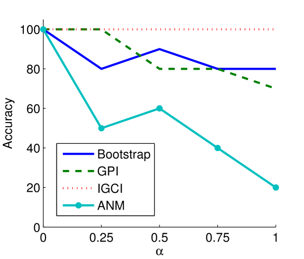
(a) Changing $\alpha$: From additive to multiplicative noise

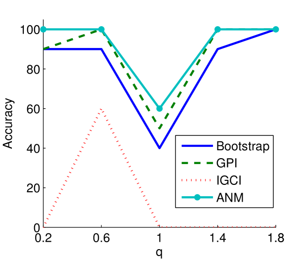
(b) Changing $q$: From sub-Gaussian to super-Gaussian additive noise

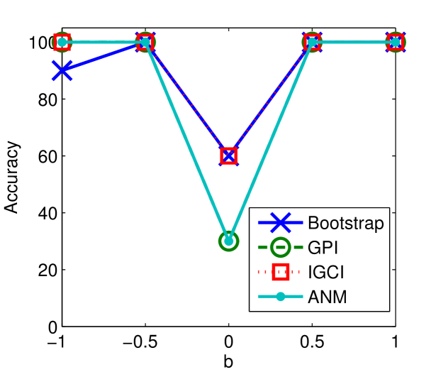
(c) Changing $b$: Various nonlinear functions with Gaussian additive noise

Figure 3: Accuracy of correctly estimating the causal direction for different generating models: (a) $q=1$, $b=1$, and $\alpha$ changed from 0 to 1, (b) for a linear function ($b=0$) with additive noise ($\alpha=0$) which changed from sub-Gaussian ($q<1$) to sub-Gaussian ($q>1$), and (c) various nonlinear functions ($b$ changed from -1 to 1) with additive Gaussian noise ($q=1$, $\alpha=0$).

Simulation: Without Confounders. Inspired by the settings in [8, 15], we generated the simulated data with the model $Y=(X+bX^{3})e^{\alpha E}+(1-\alpha)E$, where $X$ and $E$ were obtained by passing i.i.d. Gaussian samples through power nonlinearities with exponent $q$, while keeping the original signs. The parameter $\alpha$ controls the type of the observation noise, ranging from purely additive noise ($\alpha=0$) to purely multiplicative noise ($\alpha=1$). $b$ determines how nonlinear the effect of $X$ is, and when $b=0$ the model is linear. The parameter $q$ controls the non-Gaussninity of $X$ and $E$: $q=1$ corresponds to a Gaussian distribution, and $q>1$ and $q<1$ produce super-Gaussian and sub-Gaussian distributions, respectively.

We considered three situations, in each of which two of $q$, $b$, and $\alpha$ were fixed and we see how the other changes the performance of different methods. For each combination of $q$, $b$, and $\alpha$, we independently simulated 10 data sets with 500 data points. Fig. 3 shows the accuracy of the considered methods. One can see that the accuracy of the bootstrap-based approach is among or close to the best results, indicating that it is able to perform causal inference in various situations. We note that in practice, the performance of the bootstrap-based approach depends on the number of bootstrap replications and the method used for conditional distribution estimation. Although due to computatioanl reasons, we did not try a larger number of bootstrap replications, generally speaking, the accuracy of the bootstrap-based method improves as the number of replications increases.

Simulation: With Confounders. We then include the confounder variable $Z$ in the system, so that the causal structure is $Z\rightarrow X$ and $(Z,X)\rightarrow Y$. For simplicity, we assume that both $X$ and $Y$ are influenced by $Z$ in a linear form: $X=(2-\beta)E_{X}+\beta Z$, and $Y=0.3(2-\beta)\big{[}(X+bX^{3})e^{\alpha E}+(1-\alpha)E\big{]}+\beta Z$, where $E_{X}$, $Z$, and $E$ were obtained by passing i.i.d. Gaussian samples through power nonlinearities with exponent $q=1.5$, and $\beta$ controls how strong the effect of $Z$ is on both $X$ and $Y$. We considered two situations: in one of them, we set $\alpha=0$ and $b=0$, i.e., the whole model is linear; in the other situation, $\alpha=0.2$, and $b=0.3$, so the model contains both additive noise and multiplicative noise. We changed $\beta$ from 0 to 1, and Fig. 4 shows the performances of the four methods in the two situations; note that for each value of $\beta$, the four bars (from left to right) correspond to the bootstrap-based method, GPI, IGCI, and ANM. In particular, one can see that the bootstrap-based method tends to detect the presence of the confounder when its effect is significant.

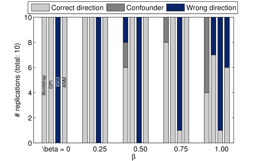
(a) Situation 1: Linear confounder case.

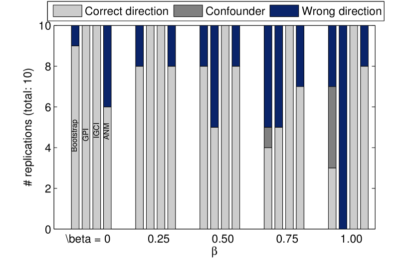
(b) Situation 2: Nonlinear confounder case.

Figure 4: Number of replications in which the methods find correct directions, report existence of confounders, and give wrong directions, respectively. For each value of $\beta$, the four bars correspond to bootstrap-based method, GPI, IGCI, and ANM (from left to right).

On Real Data. We applied the bootstrap-based method on the cause-effect pairs available at
http://webdav.tuebingen.mpg.de/cause-effect/.
To reduce computational load, we used at most 500 points for each cause-effect pair. On 20 pairs (pairs 21, 43, 45, 48-51, 56-58, 61-64, 72, 75, 77-79, and 81), the p-values of the independence test for both directions are smaller than 0.01, indicating that there might be significant confounders. This seems reasonable, as the data scatter plots for these pairs indicate that the two variables have complex dependence relationships. On the remaining 57 data sets, the bootstrap-based method output correct causal directions on 41 of them (with an accuracy 72%). We also applied the recently proposed causal inference approaches, including IGCI [10], the approach based on the Gaussian process prior [15], and that based on the post-nonlinear causal model [27] on those 57 data sets for comparison. Their performance was similar: the three approaches gave correct causal directions on 41, 40, and 43 pairs, respectively.

5 Conclusion and discussions

We proposed to do causal inference based on the criterion of exogeneity of the cause for the parameters in the conditional distribution of the effect given the cause. We discussed how to assess such exogeneity in nonparametric settings. To this end, one needs to draw a number of samples according to the unknown data-generating process. Fortunately, the bootstrap provides a way to mimic the data generating process from which we can draw a number of samples and analyze their statistical properties.

Our approach shows that it is possible to determine causal direction without structural constraints or a specific type of smoothness assumptions on the functional models. The proposed computational approach successfully demonstrated the validity of this idea, though it is computationally demanding because of the bootstrap procedure and its performance is not necessarily the best among existing methods. At the same time, it enjoys some advantages. First, it does not make a strong assumption on the data-generating process. Second, it could often tell us if significant confounders exist. The performance of the proposed bootstrap-based approach depends on the number of bootstrap replications and the method for conditional distribution estimation. In future work we aim to develop more reliable methods along this line, including methods that can handle more than two variables.

In this paper we made an attempt to discover causal information from observational data based on a condition of exogeneity, which provides another perspective to conceptualize the "independence" between the process generating the cause and that generating the effect from cause. On the other hand, it is worth mentioning that this type of independence is able to facilitate understanding and solving some machine learning or data analysis problems. For instance, it helps understand when unlabeled data points will help in the semi-supervised learning scenario [20], and inspired new settings and formulations for domain adaptation by characterizing what information to transfer and how to do so [28, 25].

Supplement to
“Distinguishing Cause from Effect Based on Exogeneity"

This supplementary material provides the proofs and discussions which are omitted in the submitted paper. The equation numbers in this material are consistent with those in the paper.
  

S1. Mutual Exogeneity and Its Relationship to Definition 1

There are two types of analysis of exogeneity [4]; one considers the inference based on the complete sample results, and the other considers dynamic models where the data were obtained by “sequential sampling". In this paper we focus on the former scenario.

From the Bayesian point of view, exogeneity of $X$ for $\psi$ allows an admissible reduction of the complete model $p(X,Y|\theta,\psi)$ to the conditional model $p(Y|X,\psi)$, in that both models lead to he same posterior distribution on the parameter set $\psi$ [4, 16]. Below we give the definition of mutual exogneneity according to [4].

Definition 3 (Mutual exogeneity)

$X$ and $\psi$ are mutually exogenous if and only if

1. $\psi$ and $X$ are independent, i.e., $\psi\mathchoice{\mathrel{\hbox to0.0pt{$\displaystyle\perp$\hss}\mkern 2.0mu{\displaystyle\perp}}}{\mathrel{\hbox to0.0pt{$\textstyle\perp$\hss}\mkern 2.0mu{\textstyle\perp}}}{\mathrel{\hbox to0.0pt{$\scriptstyle\perp$\hss}\mkern 2.0mu{\scriptstyle\perp}}}{\mathrel{\hbox to0.0pt{$\scriptscriptstyle\perp$\hss}\mkern 2.0mu{\scriptscriptstyle\perp}}}X$, and

2. $\psi$ is sufficient in the conditional distribution of $Y$ given $X$, i.e., $\theta\mathchoice{\mathrel{\hbox to0.0pt{$\displaystyle\perp$\hss}\mkern 2.0mu{\displaystyle\perp}}}{\mathrel{\hbox to0.0pt{$\textstyle\perp$\hss}\mkern 2.0mu{\textstyle\perp}}}{\mathrel{\hbox to0.0pt{$\scriptstyle\perp$\hss}\mkern 2.0mu{\scriptstyle\perp}}}{\mathrel{\hbox to0.0pt{$\scriptscriptstyle\perp$\hss}\mkern 2.0mu{\scriptscriptstyle\perp}}}Y|(\psi,X)$.

Here condition (i) is to do with the independence between $\psi$ and $X$; those two quantities play different roles in the model $p(X,Y,\psi,\theta)$, and consequently this independence condition is usually not convenient to verify. Moreover, for the same reason, there is no fully equivalent concept in sampling theory (it is weaker than exogeneity defined in Definition 1, because the property of $\theta$ is not specified). A natural way of obtaining the mutual exogeneity of $X$ and $\psi$ is to exploit a stronger but more operational condition, namely the condition of the Bayesian cut.

A Bayesian cut allows a complete separation of inference (on parameters $\theta$) in the marginal distribution and of inference (on $\psi$) in the conditional one. The prior independence between $\theta$ and $\psi$ in the Bayesian cut is a counterpart to the variation-free condition in the classical cut (condition (ii) in Definition 1), and the last two conditions in Definition 2 implies condition (i) in Definition 1. Thus, the Bayesian cut is equivalent to the classical cut in sampling theory, and consequently characterizes the exogeneity property defined in Definition 1. Therefore, hereafter the exogeneity of $X$ for $\psi$ is used interchangeably with the statement that $[\psi,(X,\theta)]$ operates a Bayesian cut in $p(X,Y,\theta,\psi)$.

The following theorem, extracted from [5], relates the Bayesian cut to the independence of the parameters according to the posterior distribution, as well as mutual exogeneity.

Theorem 4

Suppose $[\psi,(X,\theta)]$ operates a Bayesian cut in $p(X,Y,\{\psi,\theta\})$; then

• $X$ and $\psi$ are mutually exogenous, and

• $\psi$ and $\theta$ are independent a posteriori.

On the other hand, if $X$ and $\psi$ are mutually exogenous and if $\theta\mathchoice{\mathrel{\hbox to0.0pt{$\displaystyle\perp$\hss}\mkern 2.0mu{\displaystyle\perp}}}{\mathrel{\hbox to0.0pt{$\textstyle\perp$\hss}\mkern 2.0mu{\textstyle\perp}}}{\mathrel{\hbox to0.0pt{$\scriptstyle\perp$\hss}\mkern 2.0mu{\scriptstyle\perp}}}{\mathrel{\hbox to0.0pt{$\scriptscriptstyle\perp$\hss}\mkern 2.0mu{\scriptscriptstyle\perp}}}\psi|X$, $[\psi,(X,\theta)]$ operates a Bayesian cut.

When one (or more) condition in Definition 2 is violated, $[\psi,(X,\theta)]$ does not operate a Baysian cut, i.e., $X$ is not exogenous for $\psi$. Fig. 1(b–d) shows the situations where conditions (i), (ii), and (iii) are violated, respectively, so that $[\psi,(X,\theta)]$ does not operate a Baysian cut. Note that by reparameterization, the three situations can reduce to each other. Take situations (b) and (c) as an example. If we divide $\theta$ in (b) into $(\theta_{\gamma},\theta_{\mathchoice{\mathrel{\hbox to0.0pt{$\displaystyle\perp$\hss}\mkern 2.0mu{\displaystyle\perp}}}{\mathrel{\hbox to0.0pt{$\textstyle\perp$\hss}\mkern 2.0mu{\textstyle\perp}}}{\mathrel{\hbox to0.0pt{$\scriptstyle\perp$\hss}\mkern 2.0mu{\scriptstyle\perp}}}{\mathrel{\hbox to0.0pt{$\scriptscriptstyle\perp$\hss}\mkern 2.0mu{\scriptscriptstyle\perp}}}})$, where $\theta_{\gamma}$ depends on $\gamma$ while $\theta_{\mathchoice{\mathrel{\hbox to0.0pt{$\displaystyle\perp$\hss}\mkern 2.0mu{\displaystyle\perp}}}{\mathrel{\hbox to0.0pt{$\textstyle\perp$\hss}\mkern 2.0mu{\textstyle\perp}}}{\mathrel{\hbox to0.0pt{$\scriptstyle\perp$\hss}\mkern 2.0mu{\scriptstyle\perp}}}{\mathrel{\hbox to0.0pt{$\scriptscriptstyle\perp$\hss}\mkern 2.0mu{\scriptscriptstyle\perp}}}}$ does not, and consider $\theta_{\mathchoice{\mathrel{\hbox to0.0pt{$\displaystyle\perp$\hss}\mkern 2.0mu{\displaystyle\perp}}}{\mathrel{\hbox to0.0pt{$\textstyle\perp$\hss}\mkern 2.0mu{\textstyle\perp}}}{\mathrel{\hbox to0.0pt{$\scriptstyle\perp$\hss}\mkern 2.0mu{\scriptstyle\perp}}}{\mathrel{\hbox to0.0pt{$\scriptscriptstyle\perp$\hss}\mkern 2.0mu{\scriptscriptstyle\perp}}}}$ as the new $\theta$, (b) becomes (c). Similarly, if we merge $\gamma$ and $\theta$ in (c) as the new $\theta$, we then have (b). In all those situations, $\theta$ and $\psi$ are not independent a posterior, or the maximum likelihood estimates $\hat{\theta}$ and $\hat{\psi}$ are not independent according to the sampling distribution.

S2. Relation to SEM-Based Causal Inference

S2.1. Relation to Causal Inference Based on Marginal Likelihood

Recently, SEM-based approaches have demonstrated their power for causal inference of real-world problems. Structural equations represent the effect as a function of the causes and independent noise, which, from another point of view, provide a way to represent the conditional distribution $P(\texttt{effect}|\texttt{cause})$, or the causal mechanism. The generation of the cause-effect pair consists of two stages, one generating the cause according to $P(\texttt{cause})$ and the other further generating the effect from the value of the cause according to the structural equation. The “simplicity" constraints (e.g., linearity in [21], additive noise in [8], the post-nonlinear process in [27], and the smoothness assumption in [15]) on the functions are crucial. On the one hand, they make the models asymmetric in cause and effect; otherwise, for any two variables, we can always represent one of the variables as a function of the other and an independent noise term [9]. On the other hand, if the functions are constrained to be simple, the independence between the cause and the error terms would imply the exogeneity of the cause for the parameters in $P(\texttt{cause})$, as suggested by the error-based definition of exogeneity [17] (see also [18]).

The concept “exogeneity" provides theoretical support for the SEM-based causal inference methods that find the causal direction by comparing the marginal likelihood of the models in two directions; for an example of such methods, see [15]. One candidate model is given in Fig. 1(a), where $X$ is exogenous for $\psi$ (or $[\psi,(X,\psi)]$) operates a Bayesian cut in $p(X,Y,\theta,\psi)$, denoted by $\mathcal{M}_{1}$. The other corresponds to the factorization:

$$p(X,Y|\tilde{\theta},\tilde{\psi})=p(Y|\tilde{\theta})p(X|Y,\tilde{\psi}),$$ (2)

where $[\tilde{\psi},(Y,\tilde{\theta})]$ operates a Bayesian cut in $p(Y,X,\tilde{\theta},\tilde{\psi})$, denoted by $\mathcal{M}_{2}$. Note that under the above models, the marginal likelihood of $(X,Y)$ is the product of that of the conditioning variable and that of the conditional distribution. Ideally, if all the involved distributions are correctly specified, one would prefer the causal direction $X\rightarrow Y$ (resp. $Y\rightarrow X$) if $\mathcal{M}_{1}$ (resp. $\mathcal{M}_{2}$) gives a higher marginal likelihood.

Theorem 5

Suppose that the two random variables $X$ and $Y$ are generated according to $\mathcal{M}_{1}$, and that the exogeneity-based causal model is identifiable. Let the prior distributions of the parameters be $p^{*}(\psi|\mathcal{M}_{1})$ and $p^{*}(\theta|\mathcal{M}_{1})$. For the given sample $(\mathbf{X},\mathbf{Y})$, let $p(\mathbf{X},\mathbf{Y}|\mathcal{M}_{1})$ be the marginal likelihood, i.e.,

$$p(\mathbf{X},\mathbf{Y}|\mathcal{M}_{1})$$

$$= \prod_{i=1}^{N}\iint\!p({X_{i},Y_{i}}|\{\psi,\theta\})p^{*}(\theta|\mathcal{M}_{1})p^{*}(\psi|\mathcal{M}_{1})\mathrm{d}\theta\mathrm{d}\psi$$

$$= \prod_{i=1}^{N}\int\!p({X_{i}}|\theta)p^{*}(\theta|\mathcal{M}_{1})\mathrm{d}\theta\cdot\prod_{i=1}^{N}\int\!p({Y_{i}}|{X_{i}},\psi)p^{*}(\psi|\mathcal{M}_{1})\mathrm{d}\psi$$

$$= \prod_{i=1}^{N}p({X_{i}}|\mathcal{M}_{1})\cdot\prod_{i=1}^{N}p({Y_{i}}|{X_{i}},\mathcal{M}_{1}).$$

Assume that by a one-to-one reparametrization we can represent $p(X,Y|\{\psi,\theta\})$ as $p(Y|\tilde{\theta})p(X|Y,\tilde{\psi})$, where $Y$ is not exogenous for $\tilde{\psi}$. Let $p(\mathbf{X},\mathbf{Y}|\mathcal{M}_{2})$ be the marginal likelihood of $\mathcal{M}_{2}$, i.e.,

$$p(\mathbf{X},\mathbf{Y}|\mathcal{M}_{2})$$

$$= \prod_{i=1}^{N}\iint\!p({X_{i},Y_{i}}|\{\tilde{\psi},\tilde{\theta}\})p^{0}(\tilde{\theta}|\mathcal{M}_{2})p^{0}(\tilde{\psi}|\mathcal{M}_{2})\mathrm{d}\tilde{\theta}\mathrm{d}\tilde{\psi}$$

$$= \prod_{i=1}^{N}p({Y_{i}}|\mathcal{M}_{2})\cdot\prod_{i=1}^{N}p({X_{i}}|{Y_{i}},\mathcal{M}_{2}),$$

where $\tilde{\theta}$ and $\tilde{\psi}$ have independent priors. As the sample size $N$ goes to infinity, for any choice of $p^{0}(\tilde{\theta}|\mathcal{M}_{2})$ and $p^{0}(\tilde{\psi}|\mathcal{M}_{2})$, $p(\mathbf{X},\mathbf{Y}|\mathcal{M}_{1})$ is always greater than $p(\mathbf{X},\mathbf{Y}|\mathcal{M}_{2})$.

Proof 5.1.

As the data were generated according to model $\mathcal{M}_{1}$, we have

$$\mathbb{E}\log p(X,Y|\mathcal{M}_{1})=\int p(X,Y|\mathcal{M}_{1})\log p(X,Y|\mathcal{M}_{1})dxdy.$$

Furthermore,

$$\mathbb{E}\log p(X,Y|\mathcal{M}_{1})-\mathbb{E}\log p(X,Y|\mathcal{M}_{2})$$

$$= \int p(X,Y|\mathcal{M}_{1})\log\frac{p(X,Y|\mathcal{M}_{1})}{p(X,Y|\mathcal{M}_{2})}dxdy$$

$$= \mathcal{D}\big{(}p(X,Y|\mathcal{M}_{1})~{}||~{}p(X,Y|\mathcal{M}_{2})\big{)},$$

where $\mathcal{D}(\cdot||\cdot)$ denotes the Kullback-Leibler divergence. Clearly the above quantity is non-negative, and it is zero if and only if $p(X,Y|\mathcal{M}_{1})=p(X,Y|\mathcal{M}_{2})$ for all possible $x$ and $y$. However, this condition cannot hold, because the model $\mathcal{M}_{1}$ is assumed to be identifiable based on exogeneity.

Consequently, we have $\mathbb{E}\log p(X,Y|\mathcal{M}_{1})>\mathbb{E}\log p(X,Y|\mathcal{M}_{2})$. Moreover, according to the weak law of large numbers, as $N\rightarrow\infty$, $\frac{1}{N}\log p(\mathbf{X},\mathbf{Y}|\mathcal{M}_{1})$ and $\frac{1}{N}\log p(\mathbf{X},\mathbf{Y}|\mathcal{M}_{2})$ will convergence in probability to the quantities $\mathbb{E}\log p(X,Y|\mathcal{M}_{1})$ and $\mathbb{E}\log p(X,Y|\mathcal{M}_{2})$, respectively. That is, if $N$ is large enough, $p(\mathbf{X},\mathbf{Y}|\mathcal{M}_{1})>p(\mathbf{X},\mathbf{Y}|\mathcal{M}_{2})$.

However, the marginal likelihood depends heavily on the models or assumptions for the marginal and conditional distributions. Besides the exogeneity property, such approaches also make additional assumptions about the functions, such as structural constraints [21, 8, 27] and the smoothness assumption [15]. The proposed approach avoids such assumptions, by directly assessing the exogeneity property.

S2.1.1. A Simple Illustration on Parametric Models with Laplace Approximation

Here we use a somehow oversimplified parametric example to illustrate why the marginal likelihood implies the causal direction. Assume that $\mathcal{M}_{1}$ holds, that is, in factorization (1), $X$ is exogenous to $\psi$. We will demonstrate that the likelihood for model (2) would be asymptotically smaller if we wrongly assume that $Y$ is exogenous for $\tilde{\psi}$. We assume that there is a one-to-one correspondence between $(\theta,\psi)$ and $(\tilde{\theta},\tilde{\psi})$. As seen from the proof of Theorem 5, the marginal distribution of (1) under $\mathcal{M}_{1}$ would be the same as that of (2) with the dependence between $\tilde{\theta}$ and $\tilde{\psi}$ taken into account. Suppose that the corresponding log marginal likelihood $\log p(\mathbf{X},\mathbf{Y}|\mathcal{M}_{1})$, can be evaluated with the Laplace approximation in terms of $(\tilde{\theta},\tilde{\psi})$ [12]:

$$\log p(\mathbf{X},\mathbf{Y}|\mathcal{M}_{1}) \approx\log p(\mathbf{X},\mathbf{Y}|\hat{\tilde{\theta}},\hat{\tilde{\psi}})+\log p^{0}(\hat{\tilde{\theta}},\hat{\tilde{\psi}})$$

$$~{}~{}~{}~{}~{}~{}~{}~{}~{}~{}-\frac{1}{2}\log|\Sigma_{\tilde{\theta},\tilde{\psi}}|+\frac{d}{2}\log(2\pi),$$

where $\hat{\tilde{\theta}}$ and $\hat{\tilde{\psi}}$ are the maximum a posterior (MAP) estimate, $p^{0}(\hat{\tilde{\theta}},\hat{\tilde{\psi}})$ is the prior, $\Sigma_{\tilde{\theta},\tilde{\psi}}$ is the negative Hessian of $\log[p(\mathbf{X},\mathbf{Y}|\tilde{\theta},\tilde{\psi})p^{0}(\tilde{\theta})p^{0}(\tilde{\psi})]$ evaluated at $(\hat{\tilde{\theta}},\tilde{\hat{\psi}})$, and $d$ is the number of parameters.

On the other hand, under $\mathcal{M}_{2}$, the negative Hessian matrix becomes $\tilde{\Sigma}_{\tilde{\theta},\tilde{\psi}}$ which is block-diagonal and shares the same main diagonal block matrices $\Sigma_{\tilde{\theta}}$ and $\Sigma_{\tilde{\psi}}$ with $\Sigma_{\tilde{\theta},\tilde{\psi}}$. We then have $\log p(\mathbf{X},\mathbf{Y}|\mathcal{M}_{1})-\log p(\mathbf{X},\mathbf{Y}|\mathcal{M}_{2})\approx\frac{1}{2}\big{(}\log|\tilde{\Sigma}_{\tilde{\theta},\tilde{\psi}}|-\log|\Sigma_{\tilde{\theta},\tilde{\psi}}|\big{)}=\frac{1}{2}\big{(}\log|\Sigma_{\tilde{\theta}}|+\log|\Sigma_{\tilde{\psi}}|-\log|{\Sigma}_{\tilde{\theta},\tilde{\psi}}|\big{)}.$ One can show that $|{\Sigma}_{\tilde{\theta},\tilde{\psi}}|<|\Sigma_{\tilde{\theta}}|\cdot|\Sigma_{\tilde{\psi}}|$ if $\Sigma_{\tilde{\theta},\tilde{\psi}}$ is not block-diagonal; for a proof, see [1, page 239]. Hence, we have $\log p(\mathbf{X},\mathbf{Y}|\mathcal{M}_{1})>\log p(\mathbf{X},\mathbf{Y}|\mathcal{M}_{2})$ asymptotically.

S2.2. Relation to Invariance of SEMs

The proposed bootstrap-based method provides a way to examine if an equation is structural or not. Suppose $Y=f(X,E)$, where $E\mathchoice{\mathrel{\hbox to0.0pt{$\displaystyle\perp$\hss}\mkern 2.0mu{\displaystyle\perp}}}{\mathrel{\hbox to0.0pt{$\textstyle\perp$\hss}\mkern 2.0mu{\textstyle\perp}}}{\mathrel{\hbox to0.0pt{$\scriptstyle\perp$\hss}\mkern 2.0mu{\scriptstyle\perp}}}{\mathrel{\hbox to0.0pt{$\scriptscriptstyle\perp$\hss}\mkern 2.0mu{\scriptscriptstyle\perp}}}X$, is a structural causal model in that $f$ is invariant to changes in the distribution of $X$ [18]. One can then see that since $E$ and $X$ are independent processes, the bootstrapped $\hat{P}^{*(b)}(X)$ is independent from the underlying $\hat{p}^{*(b)}(E)$, and hence independent from $\hat{p}^{*(b)}(Y|X)=\hat{p}^{*(b)}(E)/\big{|}\frac{\partial f}{\partial E}\big{|}$.

Now consider the other direction. According to [9], we can always find an equation $X=\tilde{f}(Y;\tilde{E})$ such that $\tilde{E}\mathchoice{\mathrel{\hbox to0.0pt{$\displaystyle\perp$\hss}\mkern 2.0mu{\displaystyle\perp}}}{\mathrel{\hbox to0.0pt{$\textstyle\perp$\hss}\mkern 2.0mu{\textstyle\perp}}}{\mathrel{\hbox to0.0pt{$\scriptstyle\perp$\hss}\mkern 2.0mu{\scriptstyle\perp}}}{\mathrel{\hbox to0.0pt{$\scriptscriptstyle\perp$\hss}\mkern 2.0mu{\scriptscriptstyle\perp}}}Y$; suppose this equation is not structural, in that $\tilde{f}$, or in particular, $\big{|}\frac{\partial\tilde{f}}{\partial\tilde{E}}\big{|}$ is dependent on $p(Y)$. Again, we have $\hat{p}^{*(b)}(X|Y)=\hat{p}^{*(b)}(\tilde{E})/\big{|}\frac{\partial\tilde{f}}{\partial\tilde{E}}\big{|}$. The bootstrapped $\hat{p}^{*(b)}(Y)$ and $\hat{p}^{*(b)}(X|Y)$ are then dependent due to the dependence between $\big{|}\frac{\partial\tilde{f}}{\partial\tilde{E}}\big{|}$ and $\hat{p}^{*(b)}(Y)$.

In particular, the SEM-based causal inference approaches [21, 8, 27, 15] constrain the functions $f$ to be simple in respective senses; consequently they are not so flexible as to change with the input distribution $p(X)$, and then the independence between the input $X$ and the noise $E$ serves as a surrogate to achieve the exogeneity condition of $X$ for the parameters in $p(Y|X)$.

Compared to SEM-based approaches, the proposed exogeneity-based approach avoids the constraints on the functional causal model $f$. On the other hand, some SEM-based approaches have clear identifiability conditions under which the reverse direction $Y\rightarrow X$ that induces the same joint distribution on $(X,Y)$ does not exist in general, given the causal direction $X\rightarrow Y$; for instance, see [8, 27]. However, to find theoretical identifiability results for the proposed approach, one has to establish the identifiability conditions in terms of data distributions, which turns out to be extremely difficult.

References

- [1] W. A. Coppel. Number theory: An introduction to mathematics. Springer, second edition, 2009.
- [2] B. Efron. The Bootstrap, Jacknife and other Resampling Plans. SIAM, Philadelphia, 1982.
- [3] R. F. Engle, D. F. Hendry, and J. F. Richard. Exogeneity. Econometrica, 51:277–304, 1983.
- [4] J. P. Florens and M. Mouchart. Conditioning in dynamic models. Journal of Time Series Analysis, 6(1):15–34, 1985.
- [5] J. P. Florens, M. Mouchart, and J. M. Rolin. Elements of Bayesian Statistics. Marcel Dekker, New York, 1990.
- [6] A. Gretton, O. Bousquet, A. J. Smola, and B. Schölkopf. Measuring statistical dependence with Hilbert-Schmidt norms. In S. Jain, H.-U. Simon, and E. Tomita, editors, Algorithmic Learning Theory: 16th International Conference, pages 63–78, Berlin, Germany, 2005. Springer.
- [7] D. Henry. Econometrics: Alchemy or Science? Oxford University Press, Oxford, 2000.
- [8] P. Hoyer, D. Janzing, J. Mooji, J. Peters, and B. Schölkopf. Nonlinear causal discovery with additive noise models. In Advances in Neural Information Processing Systems 21, Vancouver, B.C., Canada, 2009.
- [9] A. Hyvärinen and P. Pajunen. Nonlinear independent component analysis: Existence and uniqueness results. Neural Networks, 12(3):429–439, 1999.
- [10] D. Janzing, J. Mooij, K. Zhang, J. Lemeire, J. Zscheischler, P. Daniuvsis, B. Steudel, and B. Schölkopf. Information-geometric approach to inferring causal directions. Artificial Intelligence, pages 1–31, 2012.
- [11] D. Janzing and B. Schölkopf. Causal inference using the algorithmic markov condition. IEEE Transactions on Information Theory, 56:5168–5194, 2010.
- [12] R. Kass, L. Tierney, and J. Kadane. Asymptotics in Bayesian computation. In J. Bernardo, M. DeGroot, D. Lindley, and A. Smith, editors, Bayesian statistics 3, pages 261–278. Oxford University Press, 1988.
- [13] N. Lawrence. Probabilistic non-linear principal component analysis with Gaussian process latent variable models. Journal of Machine Learning Research, 6:1783–1816, 2005.
- [14] E. L. Lehmann and G. Casella. Theory of point estimation. Springer, 2nd edition, 1998.
- [15] J. Mooij, O. Stegle, D. Janzing, K. Zhang, and B. Schölkopf. Probabilistic latent variable models for distinguishing between cause and effect. In Advances in Neural Information Processing Systems 23 (NIPS 2010), Curran, NY, USA, 2010.
- [16] M. Mouchart and E. Scheihing. Bayesian evaluation of non-admissible conditioning. Journal of Econometrics, 123(2):283–306, 2004.
- [17] G. H. Orcutt. Toward partial redirection of econometrics. The Review of Economics and Statistics, 34:195–200, 1952.
- [18] J. Pearl. Causality: Models, Reasoning, and Inference. Cambridge University Press, Cambridge, 2000.
- [19] J. F. Richard. Models with several regimes and changes in exogeneity. The Review of Economics Studies, 47:1–20, 1980.
- [20] B. Schölkopf, D. Janzing, J. Peters, E. Sgouritsa, K. Zhang, and J. Mooij. On causal and anticausal learning. In Proc. 29th International Conference on Machine Learning (ICML 2012), Edinburgh, Scotland, 2012.
- [21] S. Shimizu, P. Hoyer, A. Hyvärinen, and A. Kerminen. A linear non-Gaussian acyclic model for causal discovery. Journal of Machine Learning Research, 7:2003–2030, 2006.
- [22] B. W. Silverman. Density Estimation for Statistics and Data Analysis. Chapman & Hall/CRC, London, 1998.
- [23] P. Spirtes, C. Glymour, and R. Scheines. Causation, Prediction, and Search. MIT Press, Cambridge, MA, 2nd edition, 2001.
- [24] M. Sugiyama, T. Suzuki, S. Nakajima, H. Kashima, P. von Bünau, and M. Kawanabe. Direct importance estimation for covariate shift adaptation. Annals of the Institute of Statistical Mathematics, 60:699–746, 2008.
- [25] K. Zhang, , M. Gong, and B. Schölkopf. Multi-source domain adaptation: A causal view. In Proceedings of the 29th AAAI Conference on Artificial Intelligence, pages 3150–3157. AAAI Press, 2015.
- [26] K. Zhang and A. Hyvärinen. Acyclic causality discovery with additive noise: An information-theoretical perspective. In Proc. European Conference on Machine Learning and Principles and Practice of Knowledge Discovery in Databases (ECML PKDD) 2009, Bled, Slovenia, 2009.
- [27] K. Zhang and A. Hyvärinen. On the identifiability of the post-nonlinear causal model. In Proceedings of the 25th Conference on Uncertainty in Artificial Intelligence, Montreal, Canada, 2009.
- [28] K. Zhang, B. Schölkopf, K. Muandet, and Z. Wang. Domain adaptation under target and conditional shift. In Proceedings of the 30th International Conference on Machine Learning, JMLR: W&CP Vol. 28, 2013.
- [29] K. Zhang, Z. Wang, J. Zhang, and B. Schölkopf. On estimation of functional causal models: General results and application to post-nonlinear causal model. ACM Transactions on Intelligent Systems and Technologies, 2015. forthcoming.