Strong measurements give a better direct measurement of the quantum wave function

Abstract

Weak measurements have thus far been considered instrumental in the so-called direct measurement of the quantum wavefunction [Nature (London) 474, 188 (2011)]. Here we show that direct measurement of the wavefunction can be obtained by using measurements of arbitrary strength. In particular, in the case of strong measurements, i.e. those in which the coupling between the system and the measuring apparatus is maximum, we compared the precision and the accuracy of the two methods, by showing that strong measurements outperform weak measurements in both for arbitrary quantum states in most cases. We also give the exact expression of the difference between the reconstructed and original wavefunctions obtained by the weak measurement approach: this will allow to define the range of applicability of such method.

Introduction - In Quantum Mechanics the wavefunction is the fundamental representation of any quantum system, and it offers the key tool for predicting the measurement outcomes of a physical apparatus. Its determination is therefore of crucial importance in many applications. In order to reconstruct the complete quantum wavefunction of a system, an indirect method, know as quantum state tomography (QST), has been developed jame01pra . QST is based on the measurement of complementary variables of several copies of the same quantum system, followed on an estimation of the wavefunction that better reproduce the results obtained. This method, originally proposed for a two level system, has been extended to a generic number of discrete quantum states thew02pra as well as to continuous variable state lvov09rmp . Recently Lundeen et al. lund11nat proposed an alternative operational definition of the wavefunction based on the weak measurement ahar88prl ; ahar90pra ; dres14rmp . After the first demonstration, in which the transverse wavefunction of a photon has been measured, this method has been applied for the measurement of the photon polarization salv13nap , its angular momentum mali14nco and its trajectory kocs11sci . The method has been subsequently generalized to mixed states lund12prl to continuous variable systems fisc12pra and compared to standard quantum state tomography in macc14pra ; das14pra .

By such method, that we call Direct-Weak-Tomography (DWT), a “direct measurement” of the quantum wavefunction is obtained: the term “direct measurement” refers to the property that a value proportional to the wavefunction appears straight from the measured probabilities without further complicated calculations or fitting on the measurement outcomes foot1 . As originally proposed lund11nat , the method is based on the weak-measurement obtained by a “weak” interaction between the “pointer” (i.e. the measurement apparatus) and system. Weak measurements occur when the coupling between the pointer and the system is much less than the pointer width. As reported in the literature, “the crux of [the] method is that the first measurement is performed in a gentle way through weak measurement, so as not to invalidate the second”lund11nat or “Directly measuring […] relies on the technique of weak measurement: extracting so little information from a single measurement that the state does not collapse”salv13nap .

The interest about DWT is that the scheme in some cases may have experimental advantages over QST, in terms of simplicity, versatility, and directness lund12prl : it only requires a weak coupling of the system with an external pointer, a postselection of the final state of the system and a simple projective measurement of two complementary observables of the pointer, a two-level system. QST, in contrast, requires measuring a complete set of noncommuting observables of the system, which can be a very demanding requirement in systems with a large number of degrees of freedom. For instance the determination of the transverse spatial wavefunction of a single photon was first realized by DWT lund11nat , as well as the measurement of a one-million-dimensional photonic state shi15qph .

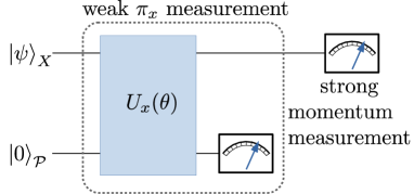
Figure 1: Scheme of the original DWT method used to measure the wavefunction.

Here we show that the quantum wavefunction can be obtained by the same scheme used in DWT, but using only strong measurements: with this terms we here refer to measurements characterized by a strong coupling between the system and the pointer. As explained below, a strong measurement does not always coincide with a projective measurement on the system.

We thus demonstrate that the weak measurement is not necessary for the direct measurement of the wavefunction. We then compare DWT with our method, showing that the use of strong measurements in most cases gives a better estimation of the quantum wavefunction, outperforming DWT when both accuracy and precision are considered. Our analysis also allows to evaluate how the wavefunction estimated by DWT is related to the correct wavefunction, see eq. (5). We also solved an unresolved question related to DWT: how “weak” the interaction should be such that DWT gives a correct estimation of the wavefunction. In particular, we will derive a sufficient criterium for the applicability of DWT based on the measured probabilities, see eq. (8).

Review of Direct-Weak-Tomography - Let’s consider a $d$ dimensional Hilbert space with basis $\{|x\rangle\}$ with $x=1,\dots,d$. The states $|x\rangle$ are equivalent to position eigenstates of a discretized segment. A generic pure state in this basis can be written as

$${|\psi\rangle}_{X}=\sum^{d}_{x=1}\psi_{x}|x\rangle\,.$$ (1)

The scheme used in DWT is shown in figure 1: first, the following initial state $|\Psi_{\rm in}\rangle={|\psi\rangle}_{X}\otimes{|0\rangle}_{\mathcal{P}}$ is prepared, with ${|0\rangle}_{\mathcal{P}}$ the pointer state. The pointer belongs to a bidimensional qubit space spanned by the states $\{{|0\rangle}_{\mathcal{P}},{|1\rangle}_{\mathcal{P}}\}$ foot2 . The system is then evolved according to the following unitary operator:

$$U_{x}(\theta) =e^{-i\theta\hat{\pi}_{x}\otimes\hat{\sigma}_{y}}\approx\openone-i\theta\,\hat{\pi}_{x}\otimes\hat{\sigma}_{y}\,,$$ (2)

where $\theta$ is an arbitrary angle and $\hat{\pi}_{x}=|x\rangle\langle x|$. The approximation of the r.h.s. of eq. (2) is obtained for small $\theta$. The previous evolution corresponds to a pointer rotation conditioned to $|\psi\rangle_{X}$ being in the state $|x\rangle$. A projective measurement on the pointer, weakly coupled to the photon position and followed by a projective measurement of the photon momentum allows to directly determine the wavefunction. Indeed, by post-selecting only the outcomes corresponding to the zero transverse momentum state $|p_{0}\rangle=\frac{1}{\sqrt{d}}\sum_{x}|x\rangle$, the (unnormalized) pointer state becomes ${|\varphi\rangle}_{\mathcal{P}}\approx\frac{1}{\sqrt{d}}[\widetilde{\psi}{|0\rangle}_{\mathcal{P}}+\theta\psi_{x}{|1\rangle}_{\mathcal{P}}]$ with $\widetilde{\psi}=\sum^{d}_{x=1}\psi_{x}$. The choice of $|p_{0}\rangle$ is arbitrary, and a different value of the transverse momentum might be needed for particular states, as explained below. Since a global phase is not observable, it is possible to arbitrarily choose the phase of $\widetilde{\psi}$: we set the latter phase such that $\widetilde{\psi}$ is real valued and positive. In the first order in $\theta$, the wavefunction can be derived directly as lund11nat :

$$\psi_{W,x}=\frac{d}{2\theta\,\widetilde{\psi}}\left[(P^{(x)}_{+}-P^{(x)}_{-})+i(P^{(x)}_{L}-P^{(x)}_{R})\right]\,,$$ (3)

where $P^{(x)}_{j}$ represent the probabilities of measuring the pointer state into the diagonal basis ${|\pm\rangle}_{\mathcal{P}}=\frac{1}{\sqrt{2}}(|0\rangle\pm|1\rangle)$, or the circular basis ${|L\rangle}_{\mathcal{P}}=\frac{1}{\sqrt{2}}(|0\rangle+i|1\rangle)$ and ${|R\rangle}_{\mathcal{P}}=\frac{1}{\sqrt{2}}(|0\rangle-i|1\rangle)$. We note that, since the (real positive) proportionality constant $\frac{d}{2\theta\widetilde{\psi}}$ is $x$ independent, it can be obtained at the end of the procedure by normalizing the wavefunction. The different probabilities can be also expressed in the framework of POVM, as detailed is SI. From now on, we indicate with $\psi_{W,x}$ the (approximate) wavefunction obtained with the DWT method. We also define $\widetilde{\psi}_{W}\equiv\sum_{x}\psi_{W,x}=\frac{d}{2\theta\,\widetilde{\psi}}\sum_{x}(P^{(x)}_{+}-P^{(x)}_{-})$ and we fix the global phase of $\psi_{W,x}$ by (3).

Relation (3) was generalized to mixed states in lund12prl . By repeating the measurements and changing the $x$ parameter in the evolution $U_{x}(\theta)$, the full wavefunction can be reconstructed. We now show that a relation similar to (3) can be obtained by strong or arbitrary strength measurements.

Arbitrary strength measurement - Measurement with arbitrary strength is obtained by choosing arbitrary value of $\theta$ within $0<\theta\leq\pi/2$. We start our analysis with strong measurements, corresponding to $\theta=\pi/2$. In this case the unitary operator (2) becomes $U_{x}(\pi/2)=\openone-|x\rangle\langle x|\otimes(\openone_{\pi}+i\sigma_{y})$. After the interaction, the initial state $|\Psi_{\rm in}\rangle$ is measured on the state $|p_{0}\rangle\otimes|\phi_{f}\rangle$, where $|\phi_{f}\rangle$ is the final polarization state. The amplitude for that transition is just $\mathcal{A}=\langle p_{0}|\psi\rangle_{X}\langle\phi_{f}|0\rangle_{\mathcal{P}}-\psi_{x}\sqrt{2/d}\langle\phi_{f}|-\rangle_{\mathcal{P}}$. This amplitude involves both the real and imaginary parts of $\psi_{x}$, so its magnitude squared does too: by choosing different values of $|\psi_{f}\rangle$, it is possible to determine the real and imaginary parts of $\psi_{x}$. In particular by choosing the final state $|\phi_{f}\rangle$ as ${|1\rangle}_{\mathcal{P}}$, ${|+\rangle}_{\mathcal{P}}$, ${|-\rangle}_{\mathcal{P}}$, ${|L\rangle}_{\mathcal{P}}$ and ${|R\rangle}_{\mathcal{P}}$ states, the wavefunction can be obtained as:

$$\psi_{x} =\frac{d}{2\widetilde{\psi}}\left[(P^{(x)}_{+}-P^{(x)}_{-}+2P^{(x)}_{1})+i(P^{(x)}_{L}-P^{(x)}_{R})\right].$$ (4)

To obtain the above relation we fixed again $\widetilde{\psi}=|\widetilde{\psi}|$. It is very important to stress that, differently from the DWT method, the above result is exact, without any approximation. We denote the previous relations as Direct-Strong-Tomography (DST) method. The difference with respect to the DWT is the need of measuring the pointer state also in the state $|1\rangle_{\mathcal{P}}$. This extra requirement is compensated by the fact that the result is not approximated and the accuracy and precision of the method overcomes the DWT, as we will show in the following. We underline that the measurement in the $|1\rangle_{\mathcal{P}}$ state, and only in this state, corresponds to a projective measurement of the photon position, as the outcome of the measurement is proportional to $|\psi_{x}|^{2}$ (see S.I.). On the contrary, a projection of the pointer in the $\{|+\rangle,|-\rangle\}$ or $\{|L\rangle,|R\rangle\}$ bases acts as a partial quantum erasure on the which-position information: therefore a subsequent momentum postselection allows to extract information about the real and imaginary part of $\psi_{x}$. As detailed in SI, for arbitrary $\theta$, the wavefunction can be obtained as $\Re e(\psi_{x})\propto P^{(x)}_{+}-P^{(x)}_{-}+2\tan(\frac{\theta}{2})P^{(x)}_{1}$ and $\Im{\rm m}(\psi_{x})\propto P^{(x)}_{L}-P^{(x)}_{R}$.

Accuracy of DWT - In the case of DWT, the obtained wavefuction $\psi_{W,x}$ is an approximation of the correct wavefunction $\psi_{x}$. We now evaluate the accuracy of the DWT, namely the errors arising by using eq. (3) in place of the exact values of (4). As done in macc14pra , we define the accuracy in terms of the trace distance $\mathcal{D}$ between the correct wavefunction $\psi_{x}$ and the weak value approximation $\psi_{W,x}$ foot3 , that for pure states reduces to $\mathcal{D}=\sqrt{1-|\langle\psi|\psi_{W}\rangle|^{2}}$. We first give the analytical expression of $\mathcal{D}$ in terms of the original wave function and then show how $\mathcal{D}$ can be upper bounded by using the measurement outcomes.

As shown in SI, the relation between the exact wavefunction $\psi_{x}$ and the weak-value estimate $\psi_{W,x}$ given in (3) can be expressed by the following relation:

$$\psi_{W,x}=\psi_{x}\frac{\widetilde{\psi}-\epsilon_{\theta}\psi^{*}_{x}}{\mathcal{N}}\,,$$ (5)

with $\epsilon_{\theta}\equiv 2\sin^{2}(\frac{\theta}{2})$, $\mathcal{N}\equiv{\sqrt{|\widetilde{\psi}-\epsilon_{\theta}\langle\psi_{x}\rangle|^{2}+\epsilon_{\theta}^{2}\sigma^{2}_{\psi}}}$, and $\sigma^{2}_{\psi}\equiv\langle|\psi_{x}|^{2}\rangle-|\langle\psi_{x}\rangle|^{2}$. In the previous equation $\sigma^{2}_{\psi}$ is the “variance” of the wavefunction where the average is defined with respect the probability density $p_{x}=|\psi_{x}|^{2}$, namely $\langle|\psi_{x}|^{2}\rangle=\sum_{x}|\psi_{x}|^{4}$ and $\langle\psi_{x}\rangle=\sum_{x}\psi_{x}|\psi_{x}|^{2}$. By inserting (5) into the trace distance $\mathcal{D}$ we obtain:

$$\mathcal{D}=\frac{\epsilon_{\theta}\sigma_{\psi}}{\mathcal{N}}\,,$$ (6)

expressing $\mathcal{D}$ in terms of the original wavefunction $\psi_{x}$ and the interaction parameter $\theta$. The previous expression indicates when the weak-measurement method can be efficiently used: indeed, when

$$\mathcal{D}\ll 1\,,$$ (7)

the approximate wavefunction $\psi_{W,x}$ correctly estimates the wavefunction $\psi_{x}$. Since eq. (6) can be inverted into $\epsilon_{\theta}\sigma_{\psi}=\frac{\mathcal{D}}{\sqrt{1-D^{2}}}|\widetilde{\psi}-\epsilon_{\theta}\langle\psi_{x}\rangle|$, for small $\mathcal{D}$ condition (7) is equivalent to $\frac{\epsilon_{\theta}\sigma_{\psi}}{|\widetilde{\psi}-\epsilon_{\theta}\langle\psi_{x}\rangle|}\ll 1$ (see SI for the detailed calculation).

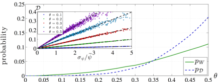
Figure 2: Accuracy of the DWT: we show the probability $p_{W}$ of having $\widetilde{\psi}_{W}<0$ and the probability $p_{\mathcal{D}}$ of having an error $\mathcal{D}$ larger that 0.1. The inset shows trace distance $\mathcal{D}$ in function of $\sigma_{\psi}/\widetilde{\psi}$ for different value of $\theta$. We randomly choose $10^{6}$ wavefunctions in a $d=10$ dimensional Hilbert space. Dashed lines in the inset represent the curves $\mathcal{D}=\epsilon_{\theta}\frac{\sigma_{\psi}}{\widetilde{\psi}}$.

Condition (7), however, cannot be used if the exact wavefunction $\psi_{x}$ is unknown. For this reason, we now present a sufficient condition for the application of DWT method that is expressed in term of the measured probabilities. As shown in SI, when the follow inequality is satisfied

$$\sum_{x}(P^{(x)}_{+}-P^{(x)}_{-})\geq 0\,,$$ (8)

the systematic error is bounded by $\mathcal{D}\leq\theta/2$ (for small $\theta$). We note that eq. (8) is equivalent to $\widetilde{\psi}_{W}\geq 0$ when the global phase of $\psi_{W,x}$ is fixed by eq. (3).

If condition (8) is not satisfied the DWT method is not guaranteed to work and a lower $\theta$ should be choosen to achieve condition (8). Since $\widetilde{\psi}_{W}$ can be expressed in term of the original wavefunction as $\widetilde{\psi}_{W}=\frac{\widetilde{\psi}^{2}-\epsilon_{\theta}}{\mathcal{N}}\,,$ for any wavefunction with $\widetilde{\psi}\neq 0$ it is possible to lower $\theta$ such that condition (8) is satisfied. The wavefunctions with $\widetilde{\psi}=0$ corresponds to the set of “pathological” wavefunctions for which the DWT and the DST methods can never be applied. Indeed, if $\widetilde{\psi}=0$ the systematic error (6) can be easily evaluated to be $\mathcal{D}=\sigma_{\psi}/\sqrt{\langle|\psi_{x}|^{2}\rangle}$ that is independent of $\theta$: by changing the interaction parameter the error cannot be lowered for such wavefunctions foot4 . Also for DST, the proportionality constant $\frac{d}{2\widetilde{\psi}\sin\theta}$ in (4) diverges if $\widetilde{\psi}=0$. In such case, a different momentum state for post-selection different from $|p_{0}\rangle$ must be used.

To better evaluate the accuracy of the DWT we have randomly chosen $10^{6}$ wavefunctions in a $d=10$ dimensional Hilbert space according to the Haar measure. We calculated for different values of $\theta$ the probability $p_{W}$ to violate the sufficient condition, namely $p_{W}={\rm Prob}(\widetilde{\psi}_{W}<0)$. We also calculated the probability $p_{\mathcal{D}}$ of having an error $\mathcal{D}$, evaluated by (6), larger that 0.1. In Figure 2 we show the probabilities $p_{W}$ and $p_{\mathcal{D}}$ in function of $\theta$. In the inset we also show the systematic error $\mathcal{D}$ in function of $\sigma_{\psi}/\widetilde{\psi}$ for different values of $\theta$. Since the distribution of $\mathcal{N}$ is peaked around $\widetilde{\psi}$ for $\theta\leq 0.5$, it is possible to approximate $\mathcal{D}\approx\epsilon_{\theta}\frac{\sigma_{\psi}}{\widetilde{\psi}}$: indeed, dashed lines in the inset of Fig. 2 represent the curves $\mathcal{D}=\epsilon_{\theta}\frac{\sigma_{\psi}}{\widetilde{\psi}}$. The figure shows that for low values of $\theta$, the DWT method fails with low probability and the systematic error is limited. Indeed, if we choose $\theta\leq 0.2$ for the $d=10$ case, we have $p_{W}\leq 1.75\%$ and $p_{\mathcal{D}}\leq 0.57\%$. Then, as expected, low values of the interaction parameter $\theta$ are suitable for the correct application of the DWT method. However, as we will show in the following, such low $\theta$ values lead to a larger statistical error (i.e. lower precision) compared to the strong measurement method.

Precision of the DWT -

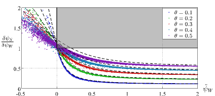
Figure 3: Ratio of statistical errors $\frac{\delta\psi_{S}}{\delta\psi_{W}}$ in function of $\widetilde{\psi}_{W}$. Shaded area represent the points in which the DWT is convenient with respect to the DST method, corresponding to $\widetilde{\psi}_{W}\geq 0$ and $\delta\psi_{W}\leq\delta\psi_{S}$.

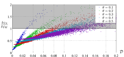
Figure 4: Ratio of statistical errors $\frac{\delta\psi_{S}}{\delta\psi_{W}}$ in function of $\mathcal{D}$. Shaded area represent the wavefuntions for which the statistical error of the DWT is lower than the DST method.

An important performance parameter is the precision of the method, namely the statistical errors on the estimated wavefunction. In particular, it is important to evaluate the scaling of such errors with the number of measurements. To this purpose, we evaluated the mean square statistical error $\delta\psi$ of the DWT and DST methods, obtained by summing the squares of the statistical error on the different $\psi_{x}$:

$$\delta\psi=\sqrt{\sum_{x}|\delta\psi_{x}|^{2}}\,.$$ (9)

As shown in SI, the ratio between the statistical errors $\delta\psi_{S}$ and $\delta\psi_{W}$, respectively corresponding to the strong and weak method, can be approximately bounded by:

$$\frac{\delta\psi_{S}}{\delta\psi_{W}}\lesssim\sin\theta_{0}\sqrt{\frac{3}{2}}\sqrt{\frac{(2d-5)\widetilde{\psi}^{2}+2\widetilde{\psi}+8-2/d}{(2d-1)\,\widetilde{\psi}^{2}+2\epsilon_{\theta}(1-\widetilde{\psi}-2\widetilde{\psi}^{2})}}$$ (10)

where $\theta_{0}$ is the interaction parameter used for the weak measurement. The terms $\sin\theta_{0}$ in eq. (10) shows that low values of $\theta_{0}$ correspond to a lower precision (i.e. larger statistical errors) of the DWT with respect to the DST method. In the statistical analysis, we compared the two method by fixing the number of repetition $N$ of the experiment: in the DWT or DST method, $N/2$ or $N/3$ repetitions are used for each basis respectively. This is the origin of the $\sqrt{3/2}$ factor in eq. (10).

For a complete demonstration of such feature we calculated the exact ratio $\frac{\delta\psi_{S}}{\delta\psi_{W}}$ for $10^{6}$ randomly chosen wavefunctions and compared it with the success parameter $\widetilde{\psi}_{W}$ and the systematic error $\mathcal{D}$. The results are shown in Fig. 3 and 4. Figure 3 show that, when the sufficiency condition for applying the DWT is satisfied, (i.e. $\widetilde{\psi}_{W}\geq 0$), the statistical errors of the DWT are typically greater then the errors of the DST. An approximate trent of the ratio ${\delta\psi_{S}}/{\delta\psi_{W}}$ can be obtained by noticing that, since $\mathcal{N}\approx\widetilde{\psi}$, we can approximate $\widetilde{\psi}_{W}\approx\widetilde{\psi}-\epsilon_{\theta}/\widetilde{\psi}$. Dashed curves in Fig. 3 represent the r.h.s. of eq. (10), with $\widetilde{\psi}$ replaced by $\frac{1}{2}(\widetilde{\psi}_{W}+\sqrt{\widetilde{\psi}^{2}_{W}+4\epsilon_{\theta}})$ and well reproduce the behavior of the ratio $\delta\psi_{S}/\delta\psi_{W}$.

To further prove that the DST precision is typically greater than the DWT one, we plot in Fig. 4 the same ratio $\delta\psi_{S}/\delta\psi_{W}$ in function of the exact trace distance $\mathcal{D}$: for low systematic error $\mathcal{D}$, the statistical errors of the DWT are typically greater then the errors of DST. Equivalently, statistical errors of the DWT are reduced only as the systematic errors increase. Fig. 4 shows that the DST precision overcomes the DWT one in most of the cases in which the DWT is accurate.

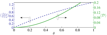
Figure 5: Mean values of $\frac{\delta\psi_{S}}{\delta\psi_{W}}$ and $\mathcal{D}$ averaged over $10^{6}$ random wavefunctions in function of $\theta$.

To better appreciate the above results, we plot in Fig. 5 the mean values of $\frac{\delta\psi_{S}}{\delta\psi_{W}}$ and $\mathcal{D}$ averaged over $10^{6}$ random wavefunctions in function of $\theta$. The plot in Fig. 5 shows again that in order to lower the trace distance $\mathcal{D}$ it is necessary to decrease $\theta$. However, decreasing $\theta$, the statistical error $\delta\psi_{W}$ becomes larger than $\delta\psi_{S}$.

Mixed states - The DWT can be generalized to determine the density matrix $\rho$ of mixed states, as shown in lund12prl . To directly measure $\rho$ the same method described for pure state can be used, with the extra requirement that the strong measurement on momentum should be performed in all the momentum states $|p\rangle=\frac{1}{\sqrt{d}}\sum_{x}e^{2\pi i\frac{px}{d}}|x\rangle$, while the pointer is measured is the $|\pm\rangle_{\mathcal{P}}$, $|R\rangle_{\mathcal{P}}$, $|L\rangle_{\mathcal{P}}$ states (as done for the pure state $|\psi\rangle_{X}$). We indicate by $\rho^{W}$ the density matrix that is reconstructed by the DWT and that approximates the correct matrix $\rho$. As shown in SI, it can be expressed as

$$\rho^{W}=\frac{1}{\cos\theta}\left[\rho+(\cos\theta-1)D\right]\,,$$ (11)

with $D$ a diagonal matrix whose element are equal to the diagonal of $\rho$, namely $D_{x,y}=\delta_{x,y}\rho_{x,x}$. By evaluating the accuracy of the DWT in terms of the trace distance $\mathcal{D}$ between $\rho$ and $\rho^{W}$ we obtained

$$\mathcal{D}=\frac{1-\cos\theta}{2\cos\theta}{\rm Tr}\left[\sqrt{(\rho-D)^{2}}\right]\,.$$ (12)

Also in this case, the larger is $\theta$, the larger is $\mathcal{D}$ and the lower is the accuracy in the estimation of $\rho$ by the DWT. Similarly to what we have shown for pure states, by performing an extra measurement of the pointer in the $|1\rangle_{\mathcal{P}}$ state, the exact expression of the density matrix can be obtained for any value of $\theta$ also in the case of mixed states (see SI).

Conclusions - We have demonstrated that, in order to achieve a direct measurement of the wavefunction, weak measurements are not necessary. Indeed, we have shown that by using strong measurements, in which a large entanglement is achieved between the system and the pointer, a better estimation of the wavefunction, in terms of precision and accuracy, can be obtained for random matrices in most cases. Our method allowed us to derive a sufficient condition for the applicability of the Direct-Weak-Tomography. We believe that our results give a deeper understanding of the meaning of the weak-value for the estimation of the wavefunction.

Appendix A Derivation of the wavefunction by generic strength measurement

We here demonstrate the relation given in eq. (4) of the main text. Let’s consider a generic interaction parameter $\theta$ and the input state $|\Psi_{\rm in}\rangle={|\psi\rangle}_{X}\otimes{|0\rangle}_{\mathcal{P}}$. In this case the unitary operators $U_{x}(\theta)$ becomes

$$U_{x}(\theta) =\openone_{x}\otimes\openone_{\pi}-|x\rangle\langle x|\otimes[(1-\cos\theta)\openone_{\pi}+i\sin\theta\sigma_{y}]\,,$$ (S1)

and the (unnormalized) pointer state after the momentum post-selection is given by

$${|\varphi\rangle}_{\mathcal{P}}=\langle p_{0}|U_{x}(\theta)|\Psi_{\rm in}\rangle =\frac{1}{\sqrt{d}}[\widetilde{\psi}|H\rangle+\psi_{x}|\chi\rangle]\,,$$ (S2)

were we have defined the (unnormalized) state $|\chi\rangle=(\cos\theta-1)|H\rangle+\sin\theta|V\rangle$ and $\widetilde{\psi}=\sum_{x}\psi_{x}$. As indicated in the main text, it is possible to choose the phase of the wave function such that $\widetilde{\psi}=|\widetilde{\psi}|$. By defining $\epsilon_{\theta}=2\sin^{2}\frac{\theta}{2}$, the probabilities of measuring in the different pointer states are given by

$$P_{0}^{(x)}= \frac{1}{d}\left[\widetilde{\psi}^{2}-2\epsilon_{\theta}\widetilde{\psi}\Re{\rm e}(\psi_{x})+\epsilon^{2}_{\theta}|\psi_{x}|^{2}\right]\approx\frac{\widetilde{\psi}^{2}}{d}$$ (S3)

$$P_{1}^{(x)}= \frac{1}{d}\sin^{2}\theta|\psi_{x}|^{2}\approx 0$$

$$P_{+}^{(x)}= \frac{1}{d}\left[\frac{\widetilde{\psi}^{2}}{2}-(\epsilon_{\theta}-\sin\theta)\widetilde{\psi}\,\Re{\rm e}(\psi_{x})+(1-\sin\theta)\epsilon_{\theta}|\psi_{x}|^{2}\right]\approx\frac{\widetilde{\psi}}{d}\left[\frac{\widetilde{\psi}}{2}+\theta\,\Re{\rm e}(\psi_{x})\right]$$

$$P_{-}^{(x)}= \frac{1}{d}\left[\frac{\widetilde{\psi}^{2}}{2}-(\epsilon_{\theta}+\sin\theta)\widetilde{\psi}\,\Re{\rm e}(\psi_{x})+(1+\sin\theta)\epsilon_{\theta}|\psi_{x}|^{2}\right]\approx\frac{\widetilde{\psi}}{d}\left[\frac{\widetilde{\psi}}{2}-\theta\,\Re{\rm e}(\psi_{x})\right]$$

$$P_{L}^{(x)}= \frac{1}{d}\left[\frac{\widetilde{\psi}^{2}}{2}+\theta\widetilde{\psi}\,\Im{\rm m}(\psi_{x})+\epsilon_{\theta}\left(|\psi_{x}|^{2}-\widetilde{\psi}\,\Re{\rm e}(\psi_{x})\right)\right]\approx\frac{\widetilde{\psi}}{d}\left[\frac{\widetilde{\psi}}{2}+\theta\Im{\rm m}(\psi_{x})\right]$$

$$P_{R}^{(x)}= \frac{1}{d}\left[\frac{\widetilde{\psi}^{2}}{2}-\sin\theta\widetilde{\psi}\,\Im{\rm m}(\psi_{x})+\epsilon_{\theta}\left(|\psi_{x}|^{2}-\widetilde{\psi}\,\Re{\rm e}(\psi_{x})\right)\right]\approx\frac{\widetilde{\psi}}{d}\left[\frac{\widetilde{\psi}}{2}-\theta\Im{\rm m}(\psi_{x})\right]$$

For low $\theta$, the approximate results of the r.h.s. holds (at the first order in $\theta$).

We note that, by defining $\alpha_{j}=\langle e_{j}|0\rangle$ and $\beta_{j}=\langle e_{j}|1\rangle$, the above probabilities can be obtained by the following POVM:

$$P_{j} ={\rm Tr}\left[E^{\dagger}_{j}E_{j}{|\psi\rangle}_{X}\langle\psi|\right]$$ (S4)

with

$$E_{j}=\alpha_{j}|p_{0}\rangle\langle p_{0}|-\gamma_{j}|p_{0}\rangle\langle x|$$ (S5)

and $\gamma_{j}=\frac{1}{\sqrt{d}}\left[(1-\cos\theta)\alpha_{j}-\sin\theta\beta_{j}\right]$.

From the previous equations (S3), using the exact results, it is possible to prove that:

$$\Re e(\psi_{x}) =\frac{d}{2\widetilde{\psi}\sin\theta}[P_{+}^{(x)}-P_{-}^{(x)}+2\tan(\frac{\theta}{2})P_{1}^{(x)}]\,,$$ (S6)

$$\Im{\rm m}(\psi_{x}) =\frac{d}{2\widetilde{\psi}\sin\theta}[P_{L}^{(x)}-P_{R}^{(x)}]\,.$$

Strong measurements correspond to $\theta=\pi/2$. By measuring the pointer in the $|e_{1}\rangle\equiv|1\rangle$, $|e_{+}\rangle\equiv|+\rangle$, $|e_{-}\rangle\equiv|-\rangle$, $|e_{L}\rangle\equiv|L\rangle$ and $|e_{R}\rangle\equiv|R\rangle$ basis, the wave function can be thus derived. It is very important to stress that the result is exact, without any approximation.

If we consider the weak-value approximation, then the approximate values of $P_{j}^{(x)}$ can be used. In this case

$$\Re{\rm e}(\psi_{W,x}) =\frac{d}{2\theta\widetilde{\psi}}(P^{(x)}_{+}-P^{(x)}_{-})$$ (S7)

$$\Im{\rm m}(\psi_{W,x}) =\frac{d}{2\theta\widetilde{\psi}}(P^{(x)}_{L}-P^{(x)}_{R})$$

Appendix B Relation between weak and strong value

Let’s now derive the the relation between the correct wave function $\psi_{x}$ and the weak-value estimate $\psi_{W,x}$. To evaluate the wave function it is necessary to estimate the parameters $A_{x}=P_{+}^{(x)}-P_{-}^{(x)}+2\tan(\frac{\theta}{2})P_{V}^{(x)}$ and $B_{x}=P_{L}^{(x)}-P_{R}^{(x)}$ such that the wavefunction is obtained by normalization:

$$\psi_{x}=\frac{A_{x}+iB_{x}}{\mathcal{M}}$$ (S8)

with $\mathcal{M}=\sqrt{\sum_{x}(A^{2}_{x}+B^{2}_{x})}=\frac{2\widetilde{\psi}\sin\theta}{d}$. On the other hand, the weak value wave function $\psi_{W,x}$ is given by

$$\psi_{W,x}=\frac{A_{W,x}+iB_{W,x}}{\mathcal{M}_{W}}$$ (S9)

with the parameters given by $A_{W,x}=P_{+}^{(x)}-P_{-}^{(x)}=\mathcal{M}[\Re{\rm e}(\psi_{x})-\frac{\epsilon_{\theta}}{\widetilde{\psi}}|\psi_{x}|^{2}]$, $B_{W,x}=P_{L}^{(x)}-P_{R}^{(x)}=\mathcal{M}\Im{\rm m}(\psi_{x})$ and $\mathcal{M}_{W}=\sqrt{\sum_{x}(A_{W,x}^{2}+B_{W,x}^{2})}$. By comparing the two results we can write

$$\psi_{W,x}=\frac{1}{\mathcal{N}}\psi_{x}(\widetilde{\psi}-\epsilon_{\theta}\psi^{*}_{x})$$ (S10)

with $\mathcal{N}$ determined by the normalization of $\psi_{W,x}$:

$$\mathcal{N} =\sqrt{\sum_{x}|\psi_{x}|^{2}|\widetilde{\psi}-\epsilon_{\theta}\psi_{x}|^{2}}=\sqrt{\widetilde{\psi}^{2}-2\epsilon_{\theta}\widetilde{\psi}\Re{\rm e}\langle\psi_{x}\rangle+\epsilon^{2}_{\theta}\langle|\psi_{x}|^{2}\rangle}$$ (S11)

$$=\sqrt{|\widetilde{\psi}-\epsilon_{\theta}\langle\psi_{x}\rangle|^{2}+\epsilon_{\theta}^{2}\sigma^{2}_{\psi}}\,.$$

The average is defined with respect the probability density defined by the wave function, $p_{x}=|\psi_{x}|^{2}$, namely $\langle|\psi_{x}|^{2}\rangle=\sum_{x}|\psi_{x}|^{4}$ and $\langle\Re{\rm e}(\psi_{x})\rangle=\sum_{x}\Re{\rm e}(\psi_{x})|\psi_{x}|^{2}$. We have thus demonstrated eq. (5) of the main text.

We now show that the trace distance between $\psi_{W,x}$ and $\psi_{x}$ can be bounded by knowing $\psi_{W,x}$. The trace distance can be exactly evaluated if we know the correct wave function $\psi_{x}$, by

$$\mathcal{D}=\frac{\epsilon_{\theta}\sigma_{\psi}}{\mathcal{N}}\,.$$ (S12)

The relation between $\mathcal{D}$ and $\epsilon_{\theta}\sigma_{\psi}$ can be inverted by squaring the previous equation, namely $\mathcal{D}^{2}=\frac{(\epsilon_{\theta}\sigma_{\psi})^{2}}{|\widetilde{\psi}-\epsilon_{\theta}\langle\psi_{x}\rangle|^{2}+(\epsilon_{\theta}\sigma_{\psi})^{2}}$. By resolving for $\epsilon_{\theta}\sigma_{\psi}$ we obtain $\epsilon_{\theta}\sigma_{\psi}=\frac{\mathcal{D}}{\sqrt{1-D^{2}}}|\widetilde{\psi}-\epsilon_{\theta}\langle\psi_{x}\rangle|$ that for low $\mathcal{D}$ can be approximated by $\epsilon_{\theta}\sigma_{\psi}\approx{\mathcal{D}}|\widetilde{\psi}-\epsilon_{\theta}\langle\psi_{x}\rangle|$, such that ${\mathcal{D}}\approx\frac{\epsilon_{\theta}\sigma_{\psi}}{|\widetilde{\psi}-\epsilon_{\theta}\langle\psi_{x}\rangle|}$. Then, for small $\mathcal{D}$, condition $\mathcal{D}\ll 1$ is equivalent to $\frac{\epsilon_{\theta}\sigma_{\psi}}{|\widetilde{\psi}-\epsilon_{\theta}\langle\psi_{x}\rangle|}\ll 1$.

The parameter $\mathcal{D}$ can be bounded by knowing $\widetilde{\psi}_{W}\equiv\sum_{x}\psi_{W,x}$. We note that the global phase of $\psi_{W,x}$ is fixed by (S10). By using (S10), we have $\widetilde{\psi}_{W}=(\widetilde{\psi}^{2}-\epsilon_{\theta})/\mathcal{N}$. When $\widetilde{\psi}_{W}\geq 0$ we can conclude that $\widetilde{\psi}\geq\sqrt{\epsilon_{\theta}}$ allowing to bound the parameter $\mathcal{D}$. Indeed, since $|\langle\psi_{x}\rangle|\leq 1$ and $\epsilon_{\theta}\leq 1$, the condition $\widetilde{\psi}\geq\sqrt{\epsilon_{\theta}}$ implies $|\widetilde{\psi}|\geq\epsilon_{\theta}|\langle\psi_{x}\rangle|$ and

$$|\widetilde{\psi}-\epsilon_{\theta}\langle\psi_{x}\rangle|^{2}\geq(\widetilde{\psi}-\epsilon_{\theta}|\langle\psi_{x}\rangle|)^{2}\geq(\widetilde{\psi}-\epsilon_{\theta})^{2}\geq\epsilon_{\theta}(1-\sqrt{\epsilon_{\theta}})^{2}\,.$$ (S13)

Finally, since $\sigma_{\psi}\leq 1/\sqrt{2}$ we can conclude that

$$\widetilde{\psi}_{W}\geq 0\qquad\Rightarrow\qquad\mathcal{D}=\frac{1}{\sqrt{\frac{|\widetilde{\psi}-\epsilon_{\theta}\langle\psi_{x}\rangle|^{2}}{\epsilon^{2}_{\theta}\sigma^{2}_{\psi}}+1}}\leq\frac{1}{\sqrt{2\frac{(1-\sqrt{\epsilon_{\theta}})^{2}}{\epsilon_{\theta}}+1}}\leq\frac{\sqrt{\epsilon_{\theta}}}{\sqrt{2-4\sqrt{\epsilon_{\theta}}+3\epsilon_{\theta}}}\approx\theta/2$$ (S14)

where the last approximate result holds for low $\theta$. The previous relation proves that the condition $\widetilde{\psi}_{W}\geq 0$ gives an upper bound on the systematic error $\mathcal{D}$. By eq. (S10) the sign of $\widetilde{\psi}_{W}$ is equal to the sign of $\sum_{x}(P^{(x)}_{+}-P^{(x)}_{-})$: then equation (S14) proves eq. (8) of the main text.

Appendix C Analysis of the precision of the DWT and DST methods

It is useful to introduce the following average error $\delta\psi$, obtained by summing the squares of the statistical error on the different $\psi_{x}$:

$$\delta\psi=\sqrt{\sum_{x}|\delta\psi_{x}|^{2}}$$ (S15)

with $|\delta\psi_{x}|^{2}=\delta\Re{\rm e}(\psi_{x})^{2}+\delta\Im{\rm m}(\psi_{x})^{2}$.

In general, for a wavefunction written as $\psi_{x}=\frac{A_{x}+iB_{x}}{\mathcal{M}}$ with $\mathcal{M}=\sqrt{\sum_{x}(A^{2}_{x}+B^{2}_{x})}$ we have

$$\delta\psi=\sqrt{\sum_{x}[(1-\frac{A_{x}^{2}}{\mathcal{M}^{2}})\delta A^{2}_{x}+(1-\frac{B_{x}^{2}}{\mathcal{M}^{2}})\delta B^{2}_{x}]}$$ (S16)

Let’s now evaluate the above expression for the two methods, the DWT and the DST.

C.1 DWT

Let’s now evaluate such average error $\delta\psi$ in the weak measurement case. Let’s consider to repeat the experiment $N$ times. For the weak value we need to measure in the $\{|L\rangle,|R\rangle\}$ and the $\{|+\rangle,|-\rangle\}$ basis. Let’s suppose that $N/2$ measurements are used for the first basis and $N/2$ per the remaining basis. We indicate with tilde the estimated parameters obtained ofter $N$ measurements. The estimate for the polarization probabilities $P_{j}$ are

$$\widetilde{P}_{j}=\frac{n_{j}}{N/2}\xrightarrow{\quad N\rightarrow\infty\quad}P_{j}$$ (S17)

since $n_{j}\rightarrow P_{j}N/2$ in the large $N$ limit. From now on we indicate with a right arrow the asymptotic behavior in the large $N$ limit. The variance of $n_{j}$ is equal to $n_{j}$ due to Poissonian statistic. Then

$$\delta\widetilde{P}_{j}=\frac{2\delta n_{j}}{N}=\frac{2\sqrt{n_{j}}}{N}\xrightarrow{\quad}\sqrt{\frac{2P_{j}}{N}}$$ (S18)

The probabilities are used to estimate the terms

$$\widetilde{A}_{W,x}=\widetilde{P}_{+}-\widetilde{P}_{-}\,,\quad\widetilde{B}_{W,x}=\widetilde{P}_{L}-\widetilde{P}_{R}\,,\quad$$ (S19)

from which the wave function is obtained in the large $N$ limit as $\Re{\rm e}(\psi_{x})=\frac{\widetilde{A}_{W,x}}{\widetilde{\mathcal{M}}_{W}}$ and $\Im{\rm m}(\psi_{x})=\frac{\widetilde{B}_{W,x}}{\widetilde{\mathcal{M}}_{W}}$ with the factor $\widetilde{\mathcal{M}}_{W}$ determined by normalization $\widetilde{\mathcal{M}}_{W}=\sqrt{\sum_{x}(\widetilde{A}^{2}_{W,x}+\widetilde{B}^{2}_{W,x})}$. In the large $N$ limit, the estimated $\widetilde{\mathcal{M}}_{W}$ approaches to $\widetilde{\mathcal{M}}_{W}\rightarrow\frac{2\sin\theta}{d}\mathcal{N}$. The statistical error on the estimated $\widetilde{A}_{x}$ and $\widetilde{B}_{x}$ are given by

$$\delta A_{W,x} =\sqrt{\delta^{2}\widetilde{P}_{+}+\delta^{2}\widetilde{P}_{-}}\xrightarrow{\quad}\sqrt{\frac{2}{dN}}\sqrt{\widetilde{\psi}^{2}-2\epsilon_{\theta}\widetilde{\psi}\Re{\rm e}(\psi_{x})+2\epsilon_{\theta}|\psi_{x}|^{2}}$$ (S20)

$$\delta B_{W,x} =\sqrt{\delta^{2}\widetilde{P}_{L}+\delta^{2}\widetilde{P}_{R}}\xrightarrow{\quad}\delta A_{W,x}$$

Since in the large $N$ limit we have $\frac{\widetilde{A}_{W,x}}{\widetilde{\mathcal{M}}_{W}}\rightarrow\Re{\rm e}(\psi_{W,x})$, $\frac{\widetilde{B}_{W,x}}{\widetilde{\mathcal{M}}_{W}}\rightarrow\Im{\rm m}(\psi_{W,x})$, the mean square statistical error $\delta\psi_{W}$ is given by

$$\delta\psi_{W}=\frac{1}{\mathcal{M}_{W}}\sqrt{\sum_{x}[(1-\Re{\rm e}(\psi_{W,x})^{2})\delta A^{2}_{W,x}+(1-\Im{\rm m}(\psi_{W,x})^{2})\delta B^{2}_{W,x}]}$$ (S21)

From (S20) we have

$$\sum_{x}(\delta A^{2}_{W,x}+\delta B^{2}_{W,x}) =\frac{2}{dN}\left[2d\,\widetilde{\psi}^{2}+4\epsilon_{\theta}(1-\widetilde{\psi}^{2})\right]$$ (S22)

$$\sum_{x}[\Re{\rm e}(\psi_{W,x})^{2}\delta A^{2}_{W,x}+\Im{\rm m}(\psi_{W,x})^{2}\delta B^{2}_{W,x}] =\frac{2}{dN}\left\{\sum_{x}|\psi_{W,x}|^{2}(\widetilde{\psi}^{2}-2\epsilon_{\theta}\widetilde{\psi}\Re{\rm e}(\psi_{x})+2\epsilon_{\theta}|\psi_{x}|^{2})\right\}$$

By using the previous equation in (S21) we obtain, for the weak value case,

$$\delta\psi_{W}\rightarrow \frac{1}{\sin\theta}\frac{1}{\mathcal{N}}\sqrt{\frac{d}{2N}}\sqrt{(2d-1)\,\widetilde{\psi}^{2}+4\epsilon_{\theta}(1-\widetilde{\psi}^{2})+2\epsilon_{\theta}\sum_{x}|\psi_{W,x}|^{2}(\widetilde{\psi}\Re{\rm e}(\psi_{x})-|\psi_{x}|^{2})}$$ (S23)

$$\geq\frac{1}{\sin\theta}\frac{1}{\mathcal{N}}\sqrt{\frac{d}{2N}}\sqrt{(2d-1)\,\widetilde{\psi}^{2}+2\epsilon_{\theta}(1-\widetilde{\psi}-2\widetilde{\psi}^{2})}$$

where we used $-\sum_{x}|\psi_{W,x}|^{2}|\psi_{x}|^{2}\geq-1$ and $\widetilde{\psi}\sum_{x}|\psi_{W,x}|^{2}\Re{\rm e}(\psi_{x})\geq-\widetilde{\psi}$.

C.2 DST

Let’s now evaluate the average error $\delta\psi$ in the strong measurement case. Again we consider to repeat the experiment $N$ times. We note that in this case we need to measure the ancillary qubit in three bases, namely $\{|L\rangle,|R\rangle\}$, $\{|+\rangle,|-\rangle\}$ and $\{|0\rangle,|1\rangle\}$ basis. Then, $N/3$ measurements are used for each basis, such that

$$\delta\widetilde{P}_{j}\xrightarrow{\quad}\sqrt{\frac{3P_{j}}{N}}\,.$$ (S24)

The $A_{x}$ and $B_{x}$ factor in eq. (S27) are given by:

$$A_{x}=\widetilde{P}_{+}-\widetilde{P}_{-}+2\tan(\frac{\theta}{2})\widetilde{P}_{V}\,,\quad B_{x}=\widetilde{P}_{L}-\widetilde{P}_{R}\,,$$ (S25)

with errors

$$\delta A_{x} =\sqrt{\delta^{2}\widetilde{P}_{+}+\delta^{2}\widetilde{P}_{-}+4\tan^{2}(\frac{\theta}{2})\delta^{2}\widetilde{P}_{V}}\xrightarrow{\quad}\sqrt{\frac{3}{Nd}}\sqrt{\widetilde{\psi}^{2}-2\epsilon_{\theta}\widetilde{\psi}\Re e(\psi_{x})+2|\psi_{x}|^{2}\epsilon_{\theta}(1+2\epsilon_{\theta})}$$ (S26)

$$\delta B_{x} =\sqrt{\delta^{2}\widetilde{P}_{L}+\delta^{2}\widetilde{P}_{R}}\xrightarrow{\quad}\sqrt{\frac{3}{dN}}\sqrt{\widetilde{\psi}^{2}-2\epsilon_{\theta}\widetilde{\psi}\Re{\rm e}(\psi_{x})+2\epsilon_{\theta}|\psi_{x}|^{2}}\,.$$

In the large $N$ limit we have $\frac{\widetilde{A}_{x}}{\widetilde{\mathcal{M}}}\rightarrow\Re{\rm e}(\psi_{x})$, $\frac{\widetilde{B}_{x}}{\widetilde{\mathcal{M}}}\rightarrow\Im{\rm m}(\psi_{x})$, and the mean square statistical error $\delta\psi$ become

$$\delta\psi=\frac{1}{\mathcal{M}}\sqrt{\sum_{x}[(1-\Re{\rm e}(\psi_{x})^{2})\delta A^{2}_{x}+(1-\Im{\rm m}(\psi_{x})^{2})\delta B^{2}_{x}]}$$ (S27)

By using (S26) we have

$$\sum_{x}(\delta A^{2}_{x}+\delta B^{2}_{x}) =\frac{3}{Nd}\left[2d\widetilde{\psi}^{2}+4\epsilon_{\theta}(1+\epsilon_{\theta}-\widetilde{\psi}^{2})\right]$$ (S28)

$$\sum_{x}[\Re{\rm e}(\psi_{x})^{2}\delta A^{2}_{x}+\Im{\rm m}(\psi_{x})^{2}\delta B^{2}_{x}] =\frac{3}{Nd}\left[\widetilde{\psi}^{2}-2\epsilon_{\theta}\widetilde{\psi}\Re e\langle\psi_{x}\rangle+2\epsilon_{\theta}\langle|\psi_{x}|^{2}\rangle+4\epsilon^{2}_{\theta}\langle\Re e(\psi_{x})^{2}\rangle\right]$$

In the large $N$ limit we have $\mathcal{M}\rightarrow\frac{2\widetilde{\psi}\sin\theta}{d}$ such that

$$\delta\psi =\frac{1}{\widetilde{\psi}\sin\theta}\sqrt{\frac{3d}{4N}}\sqrt{(2d-1)\widetilde{\psi}^{2}+4\epsilon_{\theta}(1+\epsilon_{\theta}-\widetilde{\psi}^{2})+2\epsilon_{\theta}\widetilde{\psi}\Re e\langle\psi_{x}\rangle-2\epsilon_{\theta}\langle|\psi_{x}|^{2}\rangle-4\epsilon^{2}_{\theta}\langle\Re e(\psi_{x})^{2}\rangle}$$ (S29)

For the strong measurement we have $\theta=\pi/2$ and $\epsilon_{\theta}=1$ such that

$$\delta\psi_{S} =\frac{1}{\widetilde{\psi}}\sqrt{\frac{3d}{4N}}\sqrt{(2d-5)\widetilde{\psi}^{2}+8-2\langle|\psi_{x}|^{2}\rangle-4\langle\Re e(\psi_{x})^{2}\rangle+2\widetilde{\psi}\,\langle\Re e(\psi_{x})\rangle}$$ (S30)

$$\leq\frac{1}{\widetilde{\psi}}\sqrt{\frac{3d}{4N}}\sqrt{(2d-5)\widetilde{\psi}^{2}+2\widetilde{\psi}+8-2/d}$$

since $\langle\Re e(\psi_{x})\rangle\leq 1$, $\langle|\psi_{x}|^{2}\rangle\geq\frac{1}{d}$ and $\widetilde{\psi}\leq\sqrt{d}$.

The ratio between the statistical errors can be bounded by

$$\frac{\delta\psi_{S}}{\delta\psi_{W}} \leq\sin\theta\sqrt{\frac{3}{2}}\frac{\mathcal{N}}{\widetilde{\psi}}\sqrt{\frac{(2d-5)\widetilde{\psi}^{2}+2\widetilde{\psi}+8-2/d}{(2d-1)\,\widetilde{\psi}^{2}+2\epsilon_{\theta}(1-\widetilde{\psi}-2\widetilde{\psi}^{2})}}$$ (S31)

that is the main result (eq. (9) of the main text) due to the fact that $\frac{\mathcal{N}}{\widetilde{\psi}}$ is well peaked around 1. For large $\widetilde{\psi}$ we have $\mathcal{N}\sim\widetilde{\psi}\sim\widetilde{\psi}_{W}$ and the bound is simplified to $\frac{\delta\psi_{S}}{\delta\psi_{W}}\sim\sin\theta\sqrt{\frac{3}{2}}\sqrt{\frac{2d-5}{2d-1}}$

Appendix D Mixed states with intermediate measure

Let’s consider the system initially prepared in the state

$$\rho=\rho_{X}\otimes|0\rangle_{\mathcal{P}}\langle 0|\,,\qquad{\rm with}\quad\rho_{X}=\sum\limits_{x,y=1}^{n}\hat{\rho}_{x,y}|x\rangle\langle y|$$ (S32)

and $|0\rangle_{\mathcal{P}}$ the initial “pointer” state. We would like to estimate the density matrix $\rho_{X}$. After the interaction with $U_{x}(\theta)=e^{-i\theta|x\rangle\langle x|\otimes\sigma_{y}}$, the state becomes

$$\begin{split}\rho^{\prime}_{x}\equiv U_{x}(\theta)\rho\,U^{\dagger}_{x}(\theta)\end{split}$$ (S33)

The system is then measured into the momentum state $|p\rangle=\frac{1}{\sqrt{d}}\sum\limits_{y=1}^{d}e^{\frac{2\pi iyp}{d}}|y\rangle$ such that the remaining “pointer” becomes:

$$\begin{split}\rho^{\mathcal{P}}_{x,p}\equiv\langle p|\rho^{\prime}_{x}|p\rangle=\left(\begin{matrix}\rho_{00}(x,p)&\rho_{01}(x,p)\\ \rho_{10}(x,p)&\rho_{11}(x,p)\end{matrix}\right)\end{split}$$ (S34)

with elements $\rho_{00}(x,p)=\frac{1}{d}\left[\sum_{x,y}\hat{\rho}_{x,y}e^{\frac{2\pi i(y-x)p}{d}}-2\sin^{2}\frac{\theta}{2}\sum_{y}\left(\hat{\rho}_{x,y}e^{\frac{2\pi i(y-x)p}{d}}+c.c.\right)+4\sin^{4}\frac{\theta}{2}\hat{\rho}_{x,x}\right]$, $\rho_{10}(x,p)=\frac{1}{d}\sin\theta\left[\sum_{y}\hat{\rho}_{x,y}e^{\frac{2\pi i(y-x)p}{d}}-2\sin^{2}\frac{\theta}{2}\hat{\rho}_{x,x}\right]$, $\rho_{01}(x,p)=\rho_{10}(x,p)^{*}$ and $\rho_{11}(x,p)\frac{1}{d}\sin^{2}\theta\hat{\rho}_{x,x}$.

Now it possible to determine $\hat{\rho}_{x,y}$ in function of the “pointer” density matrix as follows:

$$\hat{\rho}_{x,y}\propto d\tan\frac{\theta}{2}\delta_{x,y}\rho_{11}(x,p)+\sum_{p}e^{\frac{2\pi i(x-y)p}{d}}\rho_{10}(x,p)$$ (S35)

$$\downarrow{\rm\ strong\ measure\ }(\theta=\pi/2)$$

$$\hat{\rho}_{x,y}\propto d\delta_{x,y}\rho_{11}(x,p)+\sum_{p}e^{\frac{2\pi i(x-y)p}{d}}\rho_{10}(x,p)\,.$$ (S36)

The weak value estimate is obtained at the lowest order in $\theta$:

$$\hat{\rho}^{W}_{x,y} \propto\left[\sum_{p}e^{\frac{2\pi i(x-y)p}{d}}\rho_{10}(x,p)\right]$$ (S37)

By the above equation it is possible to express the estimated density matrix $\rho^{W}$ in terms of the correct density $\rho$ as

$$\rho^{W}=\frac{1}{\cos\theta}\left[\rho+(\cos\theta-1)D\right]$$ (S38)

with $D$ a diagonal matrix whose element are equal to the diagonal of $\rho$, namely $D_{x,y}=\delta_{x,y}\rho_{x,x}$.

To determine the terms $\rho_{10}$ in (S37) it is necessary to measure the pointer into four states $|+\rangle_{\mathcal{P}}$, $|-\rangle_{\mathcal{P}}$, $|L\rangle_{\mathcal{P}}$ and $|R\rangle_{\mathcal{P}}$. Indeed, by defining $P_{i}^{(x,p)}\equiv\langle i|\rho^{\prime\prime}_{x,p}|i\rangle$, we have the DWT relations:

$$\rho_{10}(x,p) =\frac{1}{2}\left[(P^{(x,p)}_{+}-P^{(x,p)}_{-})-i(P^{(x,p)}_{L}-P^{(x,p)}_{R})\right]$$ (S39)

The DST allows to determine the exact density matrix $\rho$ by also measuring the pointer into the state $|1\rangle_{\mathcal{P}}$. Indeed, to determine $\rho$ by eq. (S36) it is necessary to evaluate also the the terms $\rho_{11}$. It is easy to show that such terms can be evaluated by measuring the pointer into the states $|1\rangle_{\mathcal{P}}$:

$$\rho_{11}(x,p)=P^{(x,p)}_{1}\equiv P^{(x)}_{1}$$ (S40)

To summarize, for mixed states the procedure is similar to the one performed with pure state. The initial state (S32) is evolved according to the interaction $U_{x}(\theta)$ between the system and the pointer state. The system state is strongly measured in a given momentum state $|p\rangle$ such that the pointer is left into a mixed two-level system $\rho^{\mathcal{P}}_{x,p}$ given by eq. (S35). By performing a standard tomography on the pointer, namely by projecting it into $|+\rangle_{\mathcal{P}}$, $|-\rangle_{\mathcal{P}}$, $|L\rangle_{\mathcal{P}}$ and $|R\rangle_{\mathcal{P}}$ the pointer state $\rho^{\mathcal{P}}_{x,p}$ can be obtained. Then, the exact initial density matrix can be derived by eq. (S35).

References

(1)
D. F. V. James, P. G. Kwiat, W. J. Munro, and A. G. White, Phys. Rev. A
64, 052312 (2001).
(2)
R. T. Thew, K. Nemoto, A. G. White, and W. J. Munro, Phys. Rev. A 66,
012303 (2002).
(3)
A. I. Lvovsky and M. G. Raymer, Rev. Mod. Phys. 81, 299 (2009).
(4)
J. S. Lundeen, B. Sutherland, A. Patel, C. Stewart, and C. Bamber, Nature
474, 188 (2011).
(5)
Z. Shi, M. Mirhosseini, J. Margiewicz, M. Malik, F. Rivera,
R.W. Boyd, Direct measurement of a one-million-dimensional photonic state, [arXiv:1503.04713].
(6)
Y. Aharonov, D. Z. Albert, and L. Vaidman, Phys. Rev. Lett. 60, 1351
(1988).
(7)
Y. Aharonov and L. Vaidman, Phys. Rev. A 41, 11 (1990).
(8)
J. Dressel, M. Malik, F. M. Miatto, A. N. Jordan, and R. W. Boyd, Rev. Mod.
Phys. 86, 307 (2014).
(9)
J. Z. Salvail, M. Agnew, A. S. Johnson, E. Bolduc, J. Leach, and R. W. Boyd,
Nat. Photonics 7, 316 (2013).
(10)
M. Malik, M. Mirhosseini, M. P. J. Lavery, J. Leach, M. J. Padgett, and R. W.
Boyd, Nat. Comm. 5, 3115 (2014).
(11)
S. Kocsis, B. Braverman, S. Ravets, M. J. Stevens, R. P. Mirin, L. K. Shalm,
and A. M. Steinberg, Science 332, 1170 (2011).
(12)
J. S. Lundeen and C. Bamber, Phys. Rev. Lett. 108, 070402 (2012).
(13)
J. Fischbach and M. Freyberger, Phys. Rev. A 86, 052110 (2012).
(14)
L. Maccone and C. C. Rusconi, Phys. Rev. A 89, 022122 (2014).
(15)
D. Das and Arvind, Phys. Rev. A 89, 062121 (2014).
(16)
We used the
term “direct measurement” to identify the
method proposed lund11nat . As illustrated in the SI, the method can be described in the more general framework of POVMs.
(17)
In the case of photon spatial wavefunction, the pointer can be represented by
a different degrees of freedom of the photon, such as the polarization.
(18)
We here recall that
the trace distance between two quantum states and is defined as .
(19)
For example by using the DWT method on
the following wavefunction , and for the
statistical error is maximal, , for any value of .
Supplementary information: