A Bayesian approach for structure learning in oscillating regulatory networks

Abstract.

Oscillations lie at the core of many biological processes, from the cell cycle, to circadian oscillations and developmental processes. Time-keeping mechanisms are essential to enable organisms to adapt to varying conditions in environmental cycles, from day/night to seasonal. Transcriptional regulatory networks are one of the mechanisms behind these biological oscillations. However, while identifying cyclically expressed genes from time series measurements is relatively easy, determining the structure of the interaction network underpinning the oscillation is a far more challenging problem. Here, we explicitly leverage the oscillatory nature of the transcriptional signals and present a method for reconstructing network interactions tailored to this special but important class of genetic circuits. Our method is based on projecting the signal onto a set of oscillatory basis functions using a Discrete Fourier Transform. We build a Bayesian Hierarchical model within a frequency domain linear model in order to enforce sparsity and incorporate prior knowledge about the network structure. Experiments on real and simulated data show that the method can lead to substantial improvements over competing approaches if the oscillatory assumption is met, and remains competitive also in cases it is not.

1. Availability:

DSS, experiment scripts and data are available at http://homepages.inf.ed.ac.uk/gsanguin/DSS.zip

2. Contact:

D.Trejo-Banos@sms.ed.ac.uk

3. Introduction

Cyclic behaviour is ubiquitous in biology. The importance of oscillatory systems stems both from the necessity to adapt to the many environmental cycles (circadian, annual, etc.), as well as to maintain intrinsically periodic processes such as the cell cycle. Both of these type of oscillations are essential to many physiological processes, and malfunctions in the cellular time keeping mechanisms are frequently associated with disease, further motivating the study of these systems [Bell et al., 2005].

Genetic regulatory networks are at the core of many of these biological oscillators. These networks can sustain oscillatory behaviour in protein levels through specific architectures involving multiple feedback loops of transcriptional regulation. For example, a transcriptional oscillator is thought to drive the Arabidopsis thaliana circadian clock through mutual repression of three transcriptional regulators [Pokhilko et al., 2012, McClung, 2011]. The cell cycle is another oscillatory process, which controls cell division and duplication. In the case of Saccharomyces cerevisiae, experiments and dynamical models suggest that the cell cycle is the result of a transition between two self maintaining steady states, driven by two antagonistic classes of proteins [Chen et al., 2004]. Evidence suggests that a transcriptional network is an important part of this mechanism [Spellman, 1998, Li et al., 2004, Orlando et al., 2008].

These oscillators have been the subject of study for many years, but uncovering the exact mechanism is a challenge that involve many complex chemical, genetic and physiological components. It is therefore important to devise computational statistical methods which may guide experimental analyses by inferring potential regulatory interactions directly from time series gene expression data, which is usually easier to obtain.

Network inference is a well established and rich domain of research in systems biology. State of the art methods for regulatory network inference include a wide variety of techniques from statistics and machine learning. For example, mutual information between gene expression levels under different experimental conditions is used by ARACNE [Margolin et al., 2006] and CLR [Faith et al., 2007], two of the most widely used methods for network reconstruction. GENIE3 [Huynh-Thu et al., 2010], another method which was a top performer at the DREAM network inference challenges, uses random forests to produce a weighted ranking over the network edges. Other methods recently used include regularized regression [Haury et al., 2012], ANOVA [Kuffner et al., 2012] and Hierarchical Gaussian models [Li et al., 2006] Most of these methods focus on steady state data, which is by definition not available for oscillatory networks.

Regularisation-based and Bayesian methods can also be adapted to time series data. Dynamic Bayesian Networks have long been a popular choice in network inference (e.g. [Oates et al., 2012]). Such methods present considerable advantages in being able to quantify uncertainty and to incorporate prior knowledge, but are often severely limited by computational constraints. Optimisation-based methods based on regularised regression [Bonneau et al., 2006] present often a scalable alternative at the cost however of some modelling flexibility.

Here, we use a first order model of the system dynamics to constrain the network inference, but we explicitly take advantage of the oscillatory behaviour of the system by pursuing frequency-based estimation. We build a hierarchical Bayesian model over the network dynamics which can set and infer structural constraints and account for the inevitable uncertainty that experimental settings convey. Furthermore, our method can easily integrate non-trivial side information, for example in the form of sequence similarity between promoter sequence of genes. Experimental results on real and simulated data highlight that the method offers an effective and flexible platform for statistical inference in oscillatory systems, and can uncover non-trivial biological information.

The rest of the paper is organised as follows: the next section describes the methodology we use, reviewing the linear time-invariant approximation we use as well as introducing the Bayesian hierarchical framework for network inference. We then present an experimental evaluation on three data sets: a synthetic data set from the DREAM network inference challenge, a simulated data set obtained from a state of the art model of the A. thaliana circadian clock [Pokhilko et al., 2010], and a real data set from the yeast S. cerevisiae cell cycle [Orlando et al., 2008]. We then conclude the paper by discussing our method in the light of these experimental results and the existing literature on network inference.

4. Methods

Our approach is centred on the assumption that the oscillatory dynamics of the regulatory network can be reasonably approximated, in Fourier space, by a linear time invariant system. This is of course a simplification, but it is not an unreasonable one, and has been previously proposed as a formalism to model oscillatory genetic circuits with considerable success, see [Dalchau, 2011] for a recent review. From the inferential point of view, adopting a frequency domain perspective is convenient, as it enables us to transform the network reconstruction problem in a regression problem, for which many advanced estimation tools exist. We choose a Bayesian regression approach, as it provides an effective methodology to integrate diverse information in the inferential machine. As a proof of principle of how non-trivial information can be incorporated, we discuss how sequence similarity between promoter regions could be used within a hierarchical model framework.

4.1. Linear time invariant model

The starting point for our modelling is the approximation of the system’s dynamics as a Linear Time Invariant (LTI) model:

(1) $${\frac{dx_{i}\left(t\right)}{dt}=\sum_{j\neq i}^{N}\alpha_{ij}x_{j}\left(t\right)}+{{b}_{i}}-\lambda_{i}{x_{i}\left(t\right)}+\sum_{k}{c_{ik}}{{u}_{k}}.$$

Here the expression level of gene ${i}$, denoted as ${x_{i}\left(t\right)}$, depends on the expression levels of the other ${N-1}$ genes (potential regulators) through activating or repressing intensity $\alpha_{ij}\in\mathbb{R}$. Gene expression levels decay linearly with rates $\lambda_{i}$. Additionally, gene expression depends on a set of $K$ inputs ${u}_{k}$ which can be either external signals (light for example) or any other gene signal that is not modelled explicitly in the network. Finally, each gene has a basal transcription rate ${b}_{i}$.

Having a set of ${M}$ samples from an experiment (e.g. mRNA levels from a microarray experiment), let the vector $\mathbf{x}_{i}\in\mathbb{R^{M}}$ denote the set of ${M}$ expression level measurements for gene ${i}$. We can further construct the matrix $X\in\mathbb{R}^{{M}\times{N}}$, which contains the sample points for the set of ${N}$ genes. Let $\dot{X}$ be the derivative of $X$, so equation (1) in matrix form for this set of gene expression levels is given by:

(2) $$\mathrm{\dot{X}=}X{A^{T}}+\mathbf{b\mathbf{1}}+U{C^{T}}$$

where ${A}\in\mathbb{R}^{{N}\times{N}}$ is the matrix with diagonal elements $\lambda_{i}$ and off-diagonal elements $\alpha_{ij}$, the input signals are contained in matrix $U\in\mathbb{R}^{M\times K}$. To complete the notation, we denote with $\mathbf{b}$ vector of basal expression levels, which multiplies the ${M}\times{N}$ matrix of ones $\mathbf{1}$ to add a constant term to the equation.

We proceed to compute the derivative $\dot{\mathbf{x}}$ by first projecting the gene expression levels into a set of orthogonal basis functions. The chosen set of basis functions is the one given by the Discrete Fourier Transform of the gene expression levels. We emphasize that the choice of basis function is dictated by the nature of the problem: while in the limit of a continuously sampled signal this choice would be irrelevant (any complete basis would yield perfect reconstruction), for discretely sampled signals the quality of the approximation to the signal (and its derivative) will depend on the expressiveness of the chosen finite set of basis functions. Our choice of basis functions is motivated by the prior knowledge that the signals of interest should be oscillatory, making the choice to work in the frequency domain particularly appealing. We denote $\mathbf{X\left(\boldsymbol{\omega}\right)}$, $\mathbf{X}$ for brevity, as the frequency representation of $\mathbf{x}$, with each column containing the frequency spectrum of the expression of a gene over the time points. The frequency domain derivative can be computed analytically by $\mathbf{\dot{X}}=2\pi\boldsymbol{\omega}i\mathbf{X}$, so the frequency domain representation of the system is given by:

(3) $$\mathrm{\dot{\mathbf{X}}=}\mathbf{X}\mathbf{A^{T}}+\mathbf{U}\mathbf{C^{T}}.$$

Basal rates $\mathbf{b}$ are included in the zero frequency component of $\mathbf{X}$. The frequency representation of the inputs is given by $\mathbf{U}$.

To account for any discrepancies between the linearised model and the true system dynamics, we assume normally distributed error with variance $\sigma_{D}^{2}$. The likelihood function for equation (3) is:

(4) $$\begin{gathered}\mathrm{p}\left(\mathbf{\dot{X}|}\mathbf{X},\mathbf{A},\mathbf{U},\mathbf{C},\sigma_{D}\right)\propto\ \prod_{i=1}^{\mathrm{N}}\sigma_{D}^{\mathrm{-M}}\exp\left(-\frac{1}{2\sigma_{D}^{2}}\mathbf{Q_{i}}\right)\\ \mathbf{Q_{i}}=\left(\mathrm{\dot{\mathbf{X_{i}}}-}[\begin{array}[]{cc}\mathbf{X}&\mathbf{U}\end{array}]\left[\mathbf{\begin{array}[]{c}\mathbf{A_{i}^{T}}\\ \mathbf{C}_{i}^{T}\end{array}}\right]\right)^{\mathbf{T}}\mathbf{\left(\mathrm{\dot{\mathbf{X_{i}}}-}[\begin{array}[]{cc}\mathbf{X}&\mathbf{U}\end{array}]\left[\mathbf{\begin{array}[]{c}\mathbf{A_{i}^{T}}\\ \mathbf{C}_{i}^{T}\end{array}}\right]\right)}\end{gathered}.$$

In general, multiple replicate time series may be available. Denoting with ${K}$ the number of replicate time series, the overall likelihood, under an assumption of normal i.i.d error between series, can be generalized as:

(5) $$\mathrm{P}\left(\left\{\dot{\mathbf{X}}_{k}\right\}|\left\{\mathbf{X}_{k}\right\}\mathbf{A,U,C},\sigma_{D}\right)=\prod_{k=1}^{\mathrm{K}}\mathrm{P}\left(\dot{\mathbf{X}}_{k}|\mathbf{X}_{k},\mathbf{A,U,C},\sigma_{D}\right)$$

which is a product of Gaussian densities.

Notice that the form of equation (5) is identical to a regression problem where the output variables (Fourier coefficients of the derivatives of the signals) are regressed onto the Fourier coefficients of the signals. The inference problem of estimating the interaction and input response matrices $\left[\begin{array}[]{cc}\mathbf{A}^{\mathbf{T}}&\mathbf{C^{T}}\end{array}\right]^{\mathrm{T}}$ in equation (4) can therefore be attacked using the vast repertoire of regression methods. Regularized regression methods have been tested in a network inference context, see [Charbonnier et al., 2010, Bergersen et al., 2011, Bonneau et al., 2006, Haury et al., 2012]. Here, we opt for a hierarchical Bayesian approach, that will allow us to leverage prior knowledge and integrate other sources of information.

4.2. Hierarchical Bayesian modelling

To interpret dynamical systems in a network perspective, we assume that the interaction matrix in our LTI representation (1) has a sparse structure representing discrete interactions between regulators and target genes. We introduce the structural adjacency matrix $\mathbf{H}\in\mathbb{R}^{\mathrm{N}\times\mathrm{N}}$, which sits at the top of the hierarchy. This matrix contains elements $h_{ij}=1$ if gene $j$ regulates gene $i$ for $i\neq j$. In this Bayesian approach, a sparsity inducing prior over elements of $\mathbf{H}$ is necessary to aid identifiability and interpret-ability. The prior form chosen for elements $h_{ij}$ is a Bernoulli distribution, with parameter $w$ which has a Beta distribution prior due to conjugacy.

We chose a spike and slab prior to relate the connection matrix $\mathbf{H}$ and interaction matrix $\mathbf{A}$. This distribution consists of a mixture of a degenerate distribution and a long tailed distribution. The form chosen is derived from the one presented in [Ishwaran et al., 2005], where the $a_{ij}$ elements are drawn from a scale-mixture model where a zero-mean normal distribution has variance governed by hyper-parameter $\tau_{ij}$. In this form, the hyper-variance $\mathrm{h}_{ij}\tau_{ij}^{2}$ has a continuous bi-modal distribution. With this prior, the posterior distribution of the less relevant parameters is shrunk towards zero and the non-zero elements are selected by the distributions tail. The advantage of the continuous distribution implied by the scale-mixture model of [Ishwaran et al., 2005] lies primarily in the fact that we avoid the need to parametrize these bimodal distributions manually.

Thus, the hierarchical model is defined by equations:

(6) $$\begin{array}[]{ccc}{\mathrm{P}\left(\left\{\dot{\mathbf{X}}_{k}\right\}|\left\{\mathbf{X}_{k}\right\}\mathbf{A,C},\mathbf{U},\sigma_{D}\right)}&=&{\prod_{k=1}^{\mathrm{K}}\mathrm{P}\left(\dot{\mathbf{X}}_{k}|\mathbf{A,C},\mathbf{U},\mathbf{X}_{k},\sigma_{D}\right)}\\ {\mathrm{P}\left(a_{ij}|h_{ij},\tau_{ij}\right)}&\sim&\mathcal{N}\left(0,h_{ij}\tau_{ij}^{2}\right)\\ {\mathrm{P}\left(h_{ij}|w\right)}&\sim&{\left(1-w\right)\delta_{v0}+w\delta_{1}}\\ {\pi\left(w\right)}&\sim&{\mathrm{Beta}\left(\mathrm{a}_{1},\mathrm{a}_{2}\right)}\\ {\pi\left(\tau^{-2}\right)}&\sim&{\mathrm{Gamma\left(b_{1},\mathrm{b}_{2}\right)}}\\ {\pi\left(\sigma_{D}^{-2}\right)}&\sim&{\mathrm{Gamma}\left(\mathrm{c_{1},\mathrm{c}_{2}}\right)}.\end{array}$$

The parameter $\sigma_{D}$ accounts for uncertainty related to noise and model mismatch, for example arising from the linear approximation to the system dynamics. The parameter $v0$ is introduced for numerical stability and is fixed to the value of 0.005. The hyperparameters $a_{1,2}$, $b_{1,2}$ and $c_{1,2}$ can be fixed to reflect prior beliefs, or set to vague values to reflect prior ignorance; in the rest of the paper they are set to the default values of (1, 1), (5 , 50) and (0.001,0.001) respectively.

4.3. Sequence information integration

A major advantage of hierarchical modelling is the possibility of integrating different data sources. By branching from the top of the hierarchy, we can define models for different network related characteristics and keep all the information coupled by the top of the hierarchy. For example, protein interaction and binding data from ChIP-chip or ChIP-seq experiments can be used in a straightforward manner to modulate the prior probabilities over matrix $\mathbf{H}$, for example by adjusting the parameter $w$ for individual edges.

Hierarchical models also allow us to exploit more subtle sources of structural information derived from an analysis of sequence information. Transcription factors bind to the promoter region of their targets by recognizing specific motifs, short DNA words; thus co-regulated genes (genes that are regulated by a common transcription factor) should share common motifs in their promoted regions. We use this information to draw the basic model for our sequence integration approach. As the transcription binding sites share a common motif, we assume that the similarity between two promoter regions varies proportionally to the number of shared regulators. In this way, an observed pairwise similarity matrix $\mathbf{S}=[s_{ij}]$ between gene promoters, derived from a multiple alignment method like [Sievers et al., 2011] or an alignment-free method [Bonham et al., 2013], can be related to the structural adjacency matrix at the top of the hierarchical model. Assuming for simplicity a Gaussian observation model, we can then incorporate sequence similarity by positing the following relationship between promoter similarity scores and the structural adjacency matrix

(7) $$\mathrm{p}\left(s_{ij}|\mathbf{H},\boldsymbol{\beta},\sigma_{seq}\right)\propto\sigma_{seq}^{-1/2}\exp\left(-\frac{1}{2\sigma_{seq}^{2}}\left(s_{ij}-\sum_{l=1}^{\mathrm{N}}h_{il}h_{jl}\beta_{l}\right)^{2}\right)$$

Here the parameter $\left\{\beta_{l}\right\}\;1\leq l\leq N$ is the similarity “induced” by the $l-th$ transcription factor (a proportionality constant), and the product $h_{il}h_{jl}$ equals 1 if and only if genes $i$ and $j$ are both regulated by $l$. This model is a form of additive clustering [Mirkin, 1987]. By conditioning on $\mathbf{H}$, we can derive the distribution $p(\beta_{l}|...)$, which is a Gaussian with non-negative constraints, (see appendix eq. 4). This distribution can be used for sampling posterior values of $\beta$; in our applications, however, we preferred to fix the value of $\beta$ to its non-negative maximum likelihood solution, effectively approximating this conditional posterior with a $\delta$ function. The similarity score variance $\sigma_{seq}$ is given a weakly informative inverse Gamma prior. By completing the square we can derive a Gaussian distribution for the $beta_{l}$ parameters, for its derivation and estimation see appendix section 1. The overall structure of the model is depicted graphically in Fig. 1.

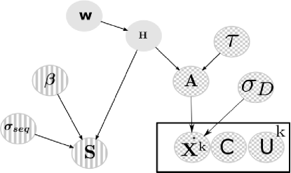
Figure 1. Hierarchical Bayesian model, on top of the hierarchy (green) lies the adjacency matrix $\mathbf{H}$ and sparsity parameter $w$. In chequered circles the frequency-domain gene expression model and its parameters. In yellow the stripes sequence similarity and its parameters.

4.4. Inference

Inference of parameters $\left\{\mathbf{A,C},\mathbf{H},\sigma_{D},w,\boldsymbol{\tau}\right\}$ is done through a simple Gibbs sampling scheme. Given conjugacy among distributions, sampling of these parameters is straightforward for all distributions except $\mathrm{p}\left(\beta_{l}\right)$. This distribution is not conjugate, so a Metropolis within Gibbs would be necessary for exact inference. In order to improve performance and given the fact that retrieving the distribution over $\beta_{l}$ is not an objective; we use the non-negative least square estimate for the vector $\boldsymbol{\beta}$. Convergence was tested by applying Geweke diagnostic over the last 1000 samples of matrix $\mathbf{H}$. Mathematical derivations of the required conditional posteriors and the general sampling algorithm are described in the appendix.

5. Results

In this section we assess the performance of our method on two realistic simulated data sets and a real data set, comparing its performance to two other state of the art methods. We call our method DSS, for DFT-based Spike and Slab model. The first simulated data set was generated from a well known model for the A. thaliana circadian clock network [Pokhilko et al., 2010]. This model is a non-linear ODE-based model which exhibits regular oscillations (for suitable parametrisations), thus matching one of our main modelling assumptions. However, it is a non-linear model, hence introducing an element of model mismatch. As a second synthetic benchmark data set we used one of the data sets provided by the DREAM 4 challenge [Marbach et al, 2010]. This is again a non-linear model, which exhibits damped oscillatory dynamics in some of the nodes; thus, this data set presents considerably more elements of model mismatch. The last experiment tested the method on a real data set of gene expression levels obtained in a micro-array experiment for the S. cerevisae cell cycle transcriptional network [Orlando et al., 2008].

Results were assessed in terms of area under the Precision-Recall (AUPR) curve; PR curves plot the fraction of correctly called instances versus the ratio of true positives over true positives plus false negatives. An ideal classifier would give a AUPR of 1, while a random baseline would return the ratio of positives negatives. Inference of the models parameters was conducted by Gibbs Sampling from the model presented in (Fig. 1) . In total, 5000 samples were obtained. The last 1000 samples were selected and averaged to compute the conditional probability of a link $\mathrm{p}\left(h_{ij}=1|\cdot\right)$ given the model and the expression data, see appendix sections 1.1.1 and 1.1.2 for details into the inputs and outputs of the program.

5.1. Competing methods

As a first comparison, in order to establish the validity of our claim that frequency domain analysis is beneficial for oscillatory networks, we sought to compare our results with a complete analogue in time domain. To do this, we implemented a spline-based alternative to the DFT, using cubic splines interpolation as means of computing the time domain derivative, while the rest of the hierarchical model was left unchanged. As competing methods to assess the performance of DSS we selected GENIE3 [Huynh-Thu et al., 2010], which is based on random forests, and the ODE-regression based Inferelator [Bonneau et al., 2006, Greenfield et al., 2013].

In a network of N genes, GENIE3 solves N regression problems by predicting, using random forests, the expression level of each gene as a function of the other N-1 genes (putative regulators). Then the relative importance of each gene expression is evaluated and the putative gene interactions are ranked. GENIE3 was designed for steady state data, but time-series adaptation can be readily derived and was provided to us by one of the authors.

The Inferelator estimates the parameters of an ODE system using regression with L1-regularization over a finite element approximation of the derivative. The method has been extended [Greenfield et al., 2013], with new functionalities to incorporate prior information over the network links, and to use alternative optimisation methods for model selection, including the elastic-net (regularization over L1 and L2 norms) and Bayesian regression with best subset selection.

Finally, as a simple baselines, we implemented a L1 regularised version of the regression problem in equation (5), using the LASSO implementation [Tibshirani, 1994].

5.2. A. thaliana circadian clock

As a first example we used data generated from a well known oscillatory network model, the A. thaliana circadian clock. The data consists of simulated mRNA measurements from the model found in [Pokhilko et al., 2010]. This non-linear model has 7 transcription factors and 2 post transcriptional elements ZTL and LHYmod. In order to replicate experimental conditions, we assume that only mRNA data is available, so protein concentrations for the transcriptional and post-transcriptional elements are assumed unobserved. The transcription factors used for network inference are ’LHY ’, ’TOC1 ’, ’PRR5 ’, hypothetical gene ’Y ’, ’GI ’, ’PRR9’ and ’PRR7’, the post-transcriptional elements are not considered. A graphical representation of the model can be observed in (appendix Fig. 1). This model was simulated for 3 cycles obtaining 28 samples. The procedure was performed with a light/dark photo period of 12/12, 6/18, 8/16, 18/6 and 20/4 hours which are represented in our model by binary input signals $\mathbf{U}$. This design of our study is created to mimic a realistic experimental setting as in [Edwards et al., 2010]; the biological rationale for such design is that stimulating the system with these different inputs may tease out the contribution of the main drivers of the clock at different times of day. We also simulated knock-out mutants $\Delta$TOC1, $\Delta$PRR7PRR9, $\Delta$LHY and $\Delta$GI by the same procedure as presented in [Pokhilko et al., 2010] with photo periods of 12/12 hours. These experiments amount to 14 time series; as these data are directly the outputs of an ODE model (without any additional noise) we define this idealised data set as the noiseless data set. An additional dataset of 14 time series was produced by adding Gaussian white noise with a Signal-to-noise (SNR) of 10. An example of the simulated expression levels is plotted in the upper left panel of Fig 2.

Using the model specification as ground truth, we proceeded to draw the PR-curves for the different methods and computed the area under the PR-curve for all the resulting networks. These areas are plotted for the noiseless (simulated data without added noise) and noisy data in the upper right panel of Fig. 2. For the case of noisy data, we generated 20 data sets by adding 10SNR-white-Gaussian noise to the noiseless data set. The simulated data has a very well defined oscillatory behaviour, as such the DSS method proved superior over the alternatives, as can be appreciated in the chart. The DSS method achieved an AUPR of 0.57 and mean 0.55 with std of 0.1 in the noisy case, being over the mean GENIE3 and Inferelator estimates with these later yielding less variance in their scores (0 variance in case of the Inferelator). The LASSO solution to the quadratic form also shows an improvement over both methods, even though DSS still has the best results. Interestingly, the spline solution achieves comparably good performance with DSS for the noiseless case, but under performs in the noisy case. We speculate that this may be due to the sensitivity of the spline estimate of the derivative to noise, confirming our intuition that adopting a set of basis functions well adapted to the problem may convey an advantage. It is intriguing that the method actually obtains a better performance on noisy data sets; we speculate that this may be due to the fact that adding noise alleviated the effects of model mismatch (resulting from the LTI approximation). Intuitively, in the absence of noise the attempts to fit non-linear data with a linear model could become more problematic.

To test the effect of including side information, we simulated a between-gene similarity matrix by drawing $\beta_{l}$ from a uniform distribution $\mathrm{U(0.1,0.6)}$ and using Equation 7. In this case we notice an important improvement by observing an increment in the AUPR to 0.68 in the noiseless case and a mean of 0.57 with std of 0.1 for the noisy data. The principal objective of using this simple simulated similarity matrix was to confirm that structural information can be retrieved and used as aid for inference. By clustering the co-regulated elements we added additional structural constraints into the inference scheme.

Finally we included a graphical representation of the true network (Fig. 2 bottom left) and a network resulting from setting a threshold of 0.5 over the inferred matrix $\mathbf{H}$ (DSS-with-similarity, noiseless data) (Fig. 2 bottom right). We notice that the 0.5 threshold, while reasonable, is still arbitrary and is used here only for the purposes of graphical visualisation. The full output from the method is a probability over the existence of edges, and can be better visualised as a heatmap, see appendix sections 1.2 and 2. Directed edges go from blue (regulators) to red (targets), black edges mean bidirectional regulation. As can be appreciated important features such as the bidirectional regulation between ’LHY’-’PRR7’ and ’LHY’-’PRR9’ are recovered. Errors are related to the roles of ’PRR7’ and ’PRR9’ regulating ’GI’ instead of ’TOC1’. This may be due to the method confounding the effects of ’TOC1’ over these former elements as being closer to the expression patterns of GI. This difficulty discriminating between the roles of the ’PRR’ genes is also expressed by inferring the spurious bidirectional edge between ’PRR7’-’PRR9’.

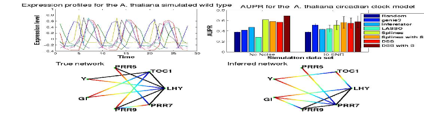
Figure 2. Top left are the simulated gene expression profiles for the wild type data set with SNR 100. Top right are the AUPR values for the 2 different noise levels. Bottom left is the true network topology, going from blue (regulators) to red (targets). Bottom right is the inferred network topology obtained by setting a threshold of 0.5 over the inferred matrix $\mathbf{H}$

5.3. DREAM Challenge

As a second example, we considered a data set from the fourth edition of the DREAM competition [Marbach et al, 2010].This data set is obtained from simulating a 10-node network, of which three nodes are input nodes; 15 regulatory links are present. Three simulations were present, one with an ODE-based system, another one with a Stochastic Differential Equation (SDE) system and a third one with SDE-based system and added experimental noise. Five time series are provided for each system, a time series contains 21 samples. The network is subjected to a single node perturbation, which mathematically corresponds to a change in the basal expression parameter, so the mean expression level of the node changes for half of the time points. The expression profiles for the set of ten genes in one time series is presented in (Fig. 3 top left). This data set does not comply with the main assumption of the model (it shows irregular damped oscillations); we therefore expect performance not to be optimal, but it is still useful to evaluate comparatively the model under such a model mismatch scenario.

Figure (Fig. 3) shows a comparison of the area under the P-curve for the three simulated systems. Of these, DSS achieves better performance in the ODE-based simulation, by having an AUPR of 0.31, higher than the nearest best method (GENIE3). Inferelator could not be executed on this data set due to numerical issues (some expression levels are exactly zero in this example). The performance improved for the SDE based simulation, by achieving an AUPR of 0.35, above inferelator’s 0.27. Slightly worse results were achieved for the SDE model with experimental noise, achieving an AUPR of 0.3. By simulating a sequence similarity matrix performance was improved for both ODE and SDE solutions. In the case of SDE the solution improved dramatically to 0.42.

As in the previous experiment, the network and its inferred counterpart are presented in Fig 3 bottom left and bottom right respectively. The inferred network is obtained by setting the threshold to 0.5 over the inferred adjacency matrix for the SDE data with added similarity matrix. As can be observed in the true network, nodes "G1" and "G10" are constant inputs. Node "G9" is subjected to perturbation for half the time points, thus its effect is propagated through the network by node "G5".

In the inferred network we can observe some interesting characteristics. First, nodes "G1" and "G9" are identified as input nodes, node "G10" is incorrectly identified as an output only node. Node "G2" maintains its out-degree of 4 even though it’s regulators are not correctly identified. Nodes "G9" and "G5" are shown with increased in and out-degree, this may also be due to the confounding effects of the their "parent-son" relationship, specially considering that the perturbed "G9" node has the biggest amplitude of the gene expression profiles, as appreciated by the red curve in the top left plot in Fig. 3.

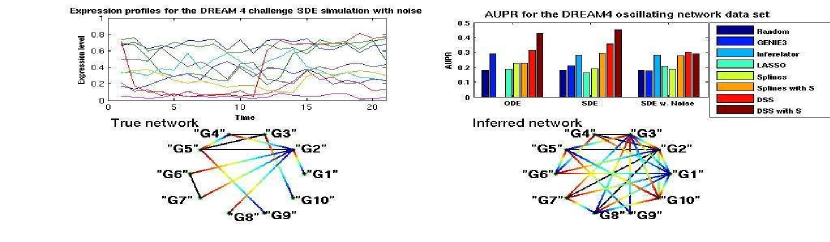
Figure 3. Top left is the expression profiles for the SDE model with experimental noise, node "G9" in red presents a perturbation over half the time points. Top right are the AUPR values for the three simulation models. Bottom left is the true network topology, from blue (regulators) to red (targets). Bottom right is the inferred network obtained by setting a threshold of 0.5 over the inferred matrix $\mathbf{H}$

5.4. S. cerevisae cell cycle

For the last experiment we used a real time series data set collected during the S. cerevisiae cell cycle. Our evaluation is based on the genes identified by [Haase et al., 2014, Orlando et al., 2008] and some of their interactions on the dynamical model found in [Chen et al., 2004]. The main transcriptional elements selected were ’SWI5’, ’YHP1’, ’SWI4’, ’FKH1’, ’SIC1’, ’ACE2’, ’YOX1’, ’STB1’, ’NRM1’, ’WHI5’, ’FKH2’, ’MCM1’, ’SWI6’, ’HCM1’, ’NDD1’ and ’MBP1’. Their putative regulations were extracted from literature {see appendix} for the putative network used as ground truth.

The source for the gene expression data is [Orlando et al., 2008], it contains 2 wild type replicates and two mutant replicates (${\Delta}clb1,2,3,4,5,6$) each one containing 14 samples for each gene during approximately 2 cell cycles. Additionally, we downloaded promoter sequence information from [Zhu et al., 1999] for all the network elements. We then proceeded to use the multiple alignment software Clustal Omega [Sievers et al., 2011] to obtain an alignment-based similarity matrix $\mathbf{S}$ between sequences. As an alternative way of encoding sequence information, an alignment-free similarity matrix $\mathbf{S2}$ was built using the method described in [Sims et al., 2009].

We tested three subsets of data, one containing only the wild type expression profiles, other containing only the mutants expression levels, the last data set was the normalized concatenation of both. As an example of the observed gene expression levels, Fig. 4 top panel shows the gene expression levels for the wild type conditions.

The AUPR from applying the various methods to this data are presented in Fig. 4 bottom left panel. In this case DSS identifies the putative network well above the random baseline of 2.1 and above the competing methods. In the case of wildtypes the AUPR of DSS was of 0.24. In the mutant data sets the performance of DSS improves by including sequence similarity achieving an AUPR of 0.2607 and 0.2608 for S and S2 respectively. The best overall performance was achieved by using the combined data set with sequence similarity matrix S2, resulting in an AUPR of 0.267.

The network in (Fig. 4) bottom right is obtained by setting the threshold of 0.9 to the inferred network from the combined wild type and mutant dataset with added similarity matrix. In this case FKH1 has a central role in the inferred network, being fully connected to the other elements. Even though this fully connected position is biologically implausible, it does reinforce the important role of FKH1 in the cell cycle, e.g. its role in regulating the M-phase response [Kumar et al., 2000]. Another noticeable inferred link concerns the post transcriptional regulation of SWI6 by WHI5p [Turner, 2012]; this regulation was also considered as part of the ground truth network, as in the case of the yeast cell cycle transcriptional and post transcriptional regulations are intertwined [Haase et al., 2014]. Also worth noticing the regulation of SWI6 by YOX1 (member of the SBF complex) even though evidence suggests causality may be in the opposite direction [Venters, 2011]. SWI4 and SWI6 form part of transcription factor complexes SBF and MBF, as such, their regulations may be confounded. This can be appreciated in the regulation of NRM1 by SWI4 in the inferred network, when in fact NRM1 appears to be regulated by SWI6 [DeJesus et al., 2013]. The transcriptional activator NDD1 is essential during the S-phase [Loy et al., 1999], NDD1p along MCM1p bind to FKH2p [Haase et al., 2014], this effect may be observable in the inferred network by directed edges from NDD1 to YOX1 and from YOX1 to FKH2.

By observing the AUPR plot we see that mutant data appears to be more informative in this case than wild type, being only marginally inferior to the combined data set with similarity matrix. Part of the experimental design in selecting mutations in [Orlando et al., 2008] was aiming at attenuating the effects of the post-transcriptional elements of the cell cycle; the stronger performance of our method on the mutant data sets may be explained by this experimental design.

Generally, the DSS solution will find the most relevant edges in the network to explain the observed dynamics, while the DSS with similarity method will find the most relevant solution that includes a grouping of the proposed edges according to the similarity matrix. So both results can be analysed separately and may offer additional insight over the whole network behaviour. With this purpose the six inferred networks and the putative ground truth are included in (appendix Fig. 3) for analysis.

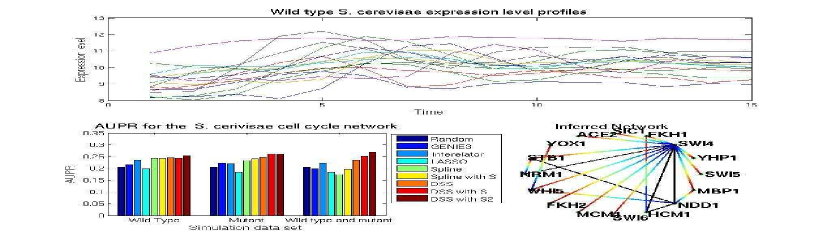
Figure 4. Top wild type yeast expression profiles for the selected genes, bottom left AUPR for the three different data combinations, wild type, mutants, and both. Bottom right network obtained by setting a threshold of 0.9 over matrix $\mathbf{H}$

6. Discussion

Inference of gene regulatory networks from expression data is one of the best studied problems in systems biology. Despite this considerable collective effort, the general problem remains ill-posed and, in the absence of extensive data sets and strong domain expertise, a solution to this problem remains elusive. In this light, it is of interest to consider more delimited problems which may be amenable to specialised but more effective solutions. Oscillatory systems present a prime example of such a problem: while they obviously constitute a specialised subset of regulatory networks, in our opinion they are sufficiently widespread to warrant tailor-made solutions. DSS couples a simplified mechanistic approach (LTI) with frequency domain information to provide such a method. LTI methods in the time domain for A. thaliana with experimental data have been studied in [Dalchau, 2011]. Our results on the circadian clock simulation suggest that this frequency domain approach can indeed be fruitful when the model assumptions are reasonably met. As Results over the DREAM and S. cerevisae data sets suggest that the method can perform competitively with state of the art methods also when the model assumptions are not precisely met (damped oscillatory behaviour); however, in these cases the methods competitive advantage is smaller or inexistent.

The use of derivative and ODE information in a network inference framework has some precedents. A method that is in spirit similar to our approach is Inferelator [Bonneau et al., 2006]. It casts the network inference problem as a a parameter inference problem over a first order differential equation system, then estimates the system parameters via regularized regression over a finite differences solution to the system. Recently Bayesian approaches that make use of the derivative information have also been proposed. In [Oates et al., 2012] a probabilistic model for integrating a linearised version of network dynamics in a regression framework is presented. [Dondelinger et al., 2013] attacked the problem of parameter inference of an ODE system jointly with a Bayesian regression over the gene expression levels. The basis of this model is a Gaussian process with product of experts likelihood, not dissimilar from our model in equation (5). However, the authors in [Dondelinger et al., 2013] did not attempt a joint parameter estimation and variable selection problem, stopping short of formulating the problem in terms of network inference. Basis functions in time domain (splines) have already been applied to network inference problems in systems biology, primarily to model unknown non-linear transition functions [Morrissey et al., 2011]. The distinctive part of our work is the proposal of a frequency domain approach for oscillatory systems, and in particular the embedding of our method within a hierarchical framework where integration of additional information is natural. We expect that non-linearities encoded as basis functions as in [Morrissey et al., 2011] would be a valuable extension of our work and likely result in an improvement in performance.

While we believe that the DSS method provides promising results, there are several inherent limitations in our approach. Importantly, the LTI approximation implies that self regulation is confounded with decay, so such types of interactions cannot be identified. Empirical results also seem to suggest that post transcriptional interactions may be confounded with transcriptional interactions; this is to be expected, as post-transcriptional interactions are not modelled in our framework. For such reasons, direct application to models that include complex post-transcriptional interactions, such as [Pokhilko et al., 2012], is not advised. Furthermore, as all Bayesian network inference methods, DSS also suffers from multi-modal posterior distributions. The use of auxiliary information, such as sequence similarity, can be beneficial to ameliorate this problem. Many different types of auxiliary information can be considered, and indeed alternative models for incorporating sequence similarity could also be used. A major strength of a Bayesian hierarchical model is that different models for auxiliary information could be easily incorporated within the DSS framework.

Appendix for A Bayesian approach for Structure learning of Oscillating Regulatory Networks

Appendix A Gibbs sampler for the Hierarchical Bayesian model.

Likelihood funcion for the LTI system.

$$\mathrm{p}\left(\mathbf{Q}_{k}|\sigma\right) \propto \sigma_{D}^{-\frac{\mathrm{M}}{2}}\exp\left(-\frac{1}{2\sigma^{-2}}\mathrm{tr}\left(\mathbf{Q}_{k}^{\mathrm{T}}\mathbf{Q}_{k}\right)\right)$$

$$\prod_{k}\mathrm{p}\left(\mathbf{Q}_{k}|\sigma\right) \propto \sigma_{D}^{-\frac{\mathrm{M+\mathrm{K}}}{2}}\exp\left(-\frac{1}{2\sigma^{-2}}\sum_{k}\mathrm{tr}\left(\mathbf{Q}_{k}^{\mathrm{T}}\mathbf{Q}_{k}\right)\right)$$

$$\mathbf{Q}_{k} = \left(\mathbf{\dot{X}}_{k}-\left[\begin{array}[]{cc}\mathbf{X}_{k}&\mathbf{U}_{k}\end{array}\right]\left[\begin{array}[]{c}\mathbf{A}^{\mathrm{T}}\\ \mathbf{C}^{\mathrm{T}}\end{array}\right]\right)$$

Conditional distribution of $\left[\begin{array}[]{c}\mathbf{A}^{\mathrm{T}}\\ \mathbf{C}^{\mathrm{T}}\end{array}\right]$

Let’s call $\mathbf{B}=$$\left[\begin{array}[]{c}\mathbf{A}^{\mathrm{T}}\\ \mathbf{C}^{\mathrm{T}}\end{array}\right]$ and $\mathbf{R}_{k}=\left[\begin{array}[]{cc}\mathbf{X}_{k}&\mathbf{U}_{k}\end{array}\right]$

$$\mathrm{p}\left(\left\{\mathbf{\dot{X}}_{k}\right\},\left\{\mathbf{R}_{\mathrm{k}}\right\}|\mathbf{B},\sigma_{D}\right) \propto \prod_{k}\mathrm{p}\left(\mathbf{\mathbf{\dot{X}}}_{k}|\mathbf{R}_{k}\mathbf{B},\sigma\right)\mathrm{p}\left(\mathbf{B}|\mathbf{H},\boldsymbol{\tau}\right)$$

$$\propto \prod_{\mathrm{k}}\exp\left(-\frac{1}{2\sigma_{D}^{2}}\mathrm{Tr}\left(-\mbox{2}\left(\mathbf{R}_{k}^{\mathrm{T}}\dot{\mathbf{X}}_{k}\right)^{\mathrm{T}}\mathbf{B}+\mathbf{B}^{\mathrm{T}}\left(\mathbf{\mathbf{R}}_{k}^{\mathrm{T}}\mathbf{R}_{k}\right)\mathbf{B}\right)\right)$$

$$\propto \exp\left(-\frac{1}{2\sigma_{D}^{2}}\mathrm{Tr}\left(-2\boldsymbol{\eta}^{\mathrm{T}}\mathbf{B}+\mathbf{B}^{\mathrm{T}}\boldsymbol{\Psi}\mathbf{B}\right)\right)$$

$$\boldsymbol{\eta}^{\mathrm{T}} = \left(\sum_{\mathrm{k}}\mathbf{R}_{k}^{\mathrm{T}}\dot{\mathbf{X}}_{k}\right)$$

$$\boldsymbol{\Psi} = \left(\sum_{\mathrm{k}}\mathbf{\mathbf{R}}_{k}^{\mathrm{T}}\mathbf{R}_{k}\right)$$

Now by using the vectorization transformation for an arbitrary matrix $\mathbf{M}$, such that $\bar{\mathbf{M}}=\mathrm{vec}\left(\mathbf{M}\right)$ and properties

$$\mathrm{Tr}\left(\mathbf{M}^{\mathrm{T}}\mathbf{N}\right) = \bar{\mathbf{M}}^{\mathrm{T}}\bar{\mathbf{N}}$$

$$\mathrm{vec}\left(\mathbf{M}\mathbf{N}\right) = \left(\mathbf{I}\otimes\mathbf{M}\right)\bar{\mathbf{N}}$$

Then we have

$$\mathrm{p}\left(\left\{\mathbf{\dot{X}}_{k}\right\},\left\{\mathbf{R}_{\mathrm{k}}\right\}|\mathbf{B},\sigma\right) \propto \exp\left(-\frac{1}{2\sigma_{D}^{2}}\left(-2\mathrm{Tr}\left(\boldsymbol{\eta}^{\mathrm{T}}\mathbf{B}\right)+\mathrm{Tr}\left(\mathbf{B}^{\mathrm{T}}\boldsymbol{\Psi}\mathbf{B}\right)\right)\right)$$

$$\propto \exp\left(-\frac{1}{2\sigma_{D}^{2}}\left(-2\bar{\boldsymbol{\eta}}^{\mathrm{T}}\bar{\mathbf{B}}+\bar{\mathbf{B}}^{\mathrm{T}}\mathrm{vec}\left(\boldsymbol{\Psi}\mathbf{B}\right)\right)\right)$$

$$\propto \exp\left(-\frac{1}{2\sigma_{D}^{2}}\left(-2\bar{\boldsymbol{\eta}}^{\mathrm{T}}\bar{\mathbf{B}}+\bar{\mathbf{B}}^{\mathrm{T}}\left(\mathbf{I}\otimes\boldsymbol{\Psi}\right)\bar{\mathbf{B}}\right)\right)$$

then by using vectorization we write the prior in canonical form

$$\mathrm{p}\left(\mathbf{B}|\mathbf{H},\boldsymbol{\tau}\right) \propto \exp\left(-\frac{1}{2}\bar{\mathbf{B}}^{\mathrm{T}}\boldsymbol{\Gamma}\bar{\mathbf{B}}\right)$$

$$\boldsymbol{\Gamma} = \mathrm{diag}\left(h_{ij}\tau_{ij}^{2}\right)$$

finally multiplying by the gaussian with hypervariance given by the spike and slab prior and completing the square we get

$$\mathrm{p}\left(\left\{\mathbf{\dot{X}}_{k}\right\},\left\{\mathbf{R}_{\mathrm{k}}\right\}|\mathbf{B},\sigma\right)\mathrm{p}\left(\mathbf{B}|\mathbf{H},\boldsymbol{\tau}\right) \propto \exp\left(-\frac{1}{2\sigma^{2}}\left(-2\bar{\boldsymbol{\eta}}^{\mathrm{T}}\bar{\mathbf{B}}+\bar{\mathbf{B}}^{\mathrm{T}}\left(\mathbf{I}\otimes\boldsymbol{\Psi}\right)\bar{\mathbf{B}}+\bar{\mathbf{B}}^{\mathrm{T}}\sigma^{2}\boldsymbol{\Gamma}\bar{\mathbf{B}}\right)\right)$$

(9) $$\mathrm{p}\left(\mathbf{B}|\left\{\mathbf{\dot{X}}_{k}\right\},\left\{\mathbf{R}_{\mathrm{k}}\right\},\mathbf{H},\boldsymbol{\tau},\sigma\right) \sim \mathcal{N}\left(\bar{\boldsymbol{\mu}},\sigma^{2}\boldsymbol{\Sigma}\right)$$

(10) $$\bar{\boldsymbol{\mu}} = \boldsymbol{\Sigma}^{-1}\bar{\boldsymbol{\eta}}^{\mathrm{T}}$$

(11) $$\boldsymbol{\Sigma^{-1}} = \mathbf{I}\otimes\boldsymbol{\Psi}+\sigma^{2}\boldsymbol{\Gamma}$$

Spike and slab prior over the coefficients

(12) $$\mathrm{p}\left(b_{ij}|h_{ij},\tau\right) \sim \mathcal{\mathcal{N}}\left(0,h_{ij}\tau_{ij}^{2}\right)$$

$$\mathrm{p}\left(h_{ij}\mathrm{|}w\right) \sim \left(1-w\right)\delta_{v0}+w\delta_{1}$$

Conditional distribution of $\tau{}^{-2}$

(13) $$\mathrm{p}\left(\tau_{ij}^{-2}|a_{ij},h_{ij}\right) \sim \mathrm{Gamma}\left(a_{1}+\frac{1}{2},a_{2}+\frac{b_{ij}^{2}}{2h_{ij}}\right)$$

Conditional distribution of $w$

(14) $$\mathrm{p}\left(w|\mathbf{H}\right)\sim\mathrm{Beta}\left(c_{1}+\#\{h_{ij}=1\},c_{2}+\#\{h_{ij}=v_{0}\}\right)$$

Condtional distribution of $\sigma_{D}^{-2}$

(15) $$\mathrm{p}\left(\sigma_{D}^{-2}|\left\{\mathbf{Q}_{k}\right\}\right)\sim\mathrm{Gamma}\left(b_{1}+\frac{\mathrm{M}\mathrm{K}}{2},b_{2}+\frac{\sum_{k}\mathrm{tr}\left(\mathbf{Q}_{k}^{\mathrm{T}}\mathbf{Q}_{k}\right)}{2}\right)$$

Likelihood of the similarity scores

(16) $$\mathrm{p}\left(s_{\mathrm{ij}}|\mathbf{H},\boldsymbol{\beta},\sigma_{seq}\right) \propto \sigma_{seq}^{-1/2}\exp\left(-\frac{1}{2\sigma_{seq}^{2}}\left(s_{ij}-\sum_{l}^{\mathrm{N}}h_{il}h_{jl}\beta_{l}\right)^{2}\right)$$

having vector$\bar{\mathbf{S}}=\left[s_{ij}\right]_{i<j}$ representing the off-diagonal elements of the upper triangular matrix of $\mathbf{S}$, vector$\mathbf{\bar{h}}_{i}$ representing the $i-th$ row vector of $\mathbf{H}$ and $\circ$ representing the elementwise product (Hadamard product). Then the distribution of the upper diagonal elements is:

$$\mathrm{p}\left(\bar{\mathbf{S}}|\mathbf{H},\boldsymbol{\beta},\sigma_{seq}\right) \propto \sigma_{seq}^{-\mathrm{D}/2}\exp\left(-\frac{1}{2\sigma_{seq}^{2}}\left(\bar{\mathbf{S}}-\left[\mathbf{\bar{h}}_{i}\circ\mathbf{\bar{h}}_{j}\right]_{i<j}\boldsymbol{\beta}\right)^{\mathrm{T}}\left(\bar{\mathbf{S}}-\left[\mathbf{\bar{h}}_{i}\circ\mathbf{\bar{h}}_{j}\right]_{i<j}\boldsymbol{\beta}\right)\right)$$

Conditional distribution for $\sigma_{seq}^{2}$

$$\mathrm{p}\left(\sigma_{seq}^{-2}|\bar{\mathbf{S}},\boldsymbol{\beta}\right) \sim \mathrm{p}\left(\bar{\mathbf{S}}|\mathbf{H},\boldsymbol{\beta},\sigma_{seq}^{-2}\right)\mathrm{p}\left(\sigma_{seq}^{-2}\right)$$

$$\sim \mathrm{Gamma}\left(a_{1}+\frac{\mathrm{D^{2}}}{2},a2+\frac{\left(\bar{\mathbf{S}}-\left[\mathbf{\bar{h}}_{i}\circ\mathbf{\bar{h}}_{j}\right]_{i<j}\boldsymbol{\beta}\right)^{\mathrm{T}}\left(\bar{\mathbf{S}}-\left[\mathbf{\bar{h}}_{i}\circ\mathbf{\bar{h}}_{j}\right]_{i<j}\boldsymbol{\beta}\right)}{2}\right)$$

Sampling $\boldsymbol{\beta}$

Instead of sampling from $\mathrm{p}\left(\beta_{l}|\centerdot\right)$ we use the non-negative least square estimate of $\boldsymbol{\beta}$, by solving the quadratic form

(18) $$\min_{\boldsymbol{\beta}}\left(\bar{\mathbf{S}}-\left[\mathbf{\bar{h}}_{i}\circ\mathbf{\bar{h}}_{j}\right]_{i<j}\boldsymbol{\beta}\right)^{\mathrm{T}}\left(\bar{\mathbf{S}}-\left[\mathbf{\bar{h}}_{i}\circ\mathbf{\bar{h}}_{j}\right]_{i<j}\boldsymbol{\beta}\right);\;s.t.\beta_{l}\geq 0$$

Conditional distribution for $h_{ij}$

We define matrices$\mathbf{H}_{ij}^{v0}=\left[\mathbf{\bar{h}}_{i}\circ\mathbf{\bar{h}}_{j}\right]_{i<j}$ such that $h_{ij}=v0$, and $\mathbf{H}_{ij}^{1}=\left[\mathbf{\bar{h}}_{i}\circ\mathbf{\bar{h}}_{j}\right]_{i<j}$ such that $h_{ij}=1$.

$$\mathrm{p}\left(h_{ij}|h_{/ij},\boldsymbol{\beta},\sigma_{seq}^{-2},\mathbf{S},\mathbf{B},w,\tau,v_{0}\right) = P\left(\mathrm{h}_{ij}\mid w\right)P\left(a_{ij}\mid h_{ij},\tau_{ij}^{2}\right)\mathrm{p}\left(\bar{\mathbf{S}}|h_{/ij},h_{ij},\boldsymbol{\beta},\sigma_{seq}\right)$$

(19) $$\mathrm{p}\left(h_{ij}|\centerdot\right) \sim \frac{m_{{}_{v0}}}{m_{{}_{v0}}+m_{1}}\left(1-w\right)\delta_{v0}+\frac{m_{1}}{m_{{}_{v0}}+m_{1}}w\delta_{1}$$

$$m_{v0} = \sigma_{seq}^{-\mathrm{D}/2}v_{0}^{-1/2}$$

$$\times \exp\left(-\frac{1}{2}\left(\frac{b_{ij}^{2}}{v_{0}\tau_{ij}^{2}}+\frac{1}{\sigma_{seq}^{2}}\left(\bar{\mathbf{S}}-\mathbf{H}_{ij}^{v0}\boldsymbol{\beta}\right)^{\mathrm{T}}\left(\bar{\mathbf{S}}-\mathbf{H}_{ij}^{v0}\boldsymbol{\beta}\right)\right)\right)$$

$$m_{1} = \sigma_{seq}^{-\mathrm{D}/2}$$

$$\times \exp\left(-\frac{1}{2}\left(\frac{b_{ij}^{2}}{\tau_{ij}^{2}}+\frac{1}{\sigma_{seq}^{2}}\left(\bar{\mathbf{S}}-\mathbf{H}_{ij}^{1}\boldsymbol{\beta}\right)^{\mathrm{T}}\left(\bar{\mathbf{S}}-\mathbf{H}_{ij}^{1}\boldsymbol{\beta}\right)\right)\right)$$

A.1. Algorithm

The Algorithm 1 presents the Gibbs sampler for parameter inference in the Hierarchical model. A brief overview of the inputs and outputs is also presented.

A.1.1. Program Inputs

Due that the DFT computed by the FFT algorithm yields complex numbers, a real representation of the coefficients is needed. We work with the so-called Real Discrete Fourier Transform. It consists of stacking the real over the imaginary part of the first $\left(M-1\right)$/2 FFT coefficients. We denote this $M\times N$ matrix $\mathbf{X}$. Figures (5) and (6) show plots for the DFT real and imaginary parts of the A. thaliana data-set, with a photoperiod of 12 hours. The magnitude and phase spectra is also shown, finally the RDFT is presented at the bottom of the picture.

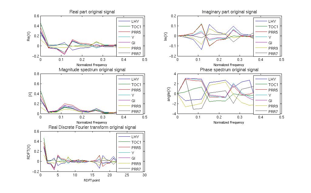
Figure 5. Spectra for the A. thaliana circadian clock simulation with a 12 hour photo-period

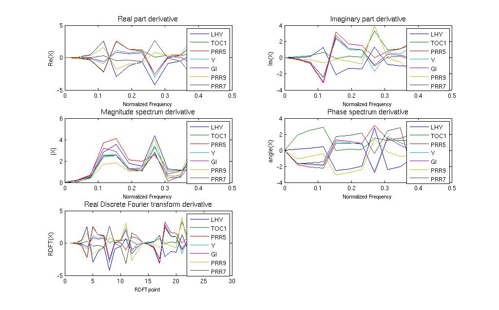
Figure 6. Derivative Spectra for the A. thaliana circadian clock simulation with a 12 hour photo-period

Hyperparameters $a_{1}$ and $a_{2}$ are set to 1 so $w$ is uniformly distributed in the interval $\left[0,1\right]$. Parameters $b_{1}$ and $b_{2}$ are set so the hypervariance $h_{ij}\tau^{2}$ has a continuos bi-modal distribution, according to the recommendations of [Ishwaran et al., 2005], in which they set them to 5 and 50 respectively. Alternative parametrization of 50 and 500 was also tested yielding better results in some cases.

The hyperparameters $c_{1}$ and $c_{2}$for$\sigma_{D}^{-2}$ are set to 0.001 and 0.001, this is a weak prior reflecting uncertainty about the linearity of the system. Hyperparamters $d_{1}$ and $d_{2}$ are set to 10 and 0.001, this parametrization required a manual tunning, as the scale parameter $\sigma_{seq}^{-2}$ having a weak prior resulted in the effects of the sequence similarity model to banish. By modifying this prior we can give more “weight” to the sequence similarity clustering thus, the flexibility of the Hierarchical model.

A.1.2. A. thaliana light inputs U

Figure 7. Three examples of light input for the A. thaliana circadian clock simulation.

A.1.3. Output

The Gibbs sampler presented in the previous section allows us to draw samples from the joint conditional distribution $p\left(\mathbf{H},\mathbf{A},\mathbf{C},\beta,w,\tau,\sigma_{D},\sigma_{s}|\left\{\mathbf{\mathbf{X}_{k}}\right\}\right)$. The marginal distribution for each of the models parameters can be drawn from this joint distribution, and the expected value for each parameter equals to the average of the samples.

For example, figure illustrates the expected value for matrix $\mathbf{H}$ obtained from averaging over 1000 samples drawn from the marginal distribution $p\left(\mathbf{H}|\left\{\mathbf{\mathbf{X}_{k}}\right\}\right)$. This figure shows in dark red those elements with higher probability of a regulatory interaction under the model assumptions, except the diagonal elements, which represent the decay rates of the equation model. The AUPR were computed by thresholding the off-diagonal elements of this matrix for each data-set.

Inputs: $K$ time series of $M$ time-points for $N$ gene expression levels, encoded in matrices $\left\{x_{k}\right\}$. Prior hyper-parameters $a_{1},a_{2},b_{1},b_{2},c_{1},c_{2}$. Optional similarity matrix $\mathbf{S}$.

Outputs: Joint conditional posterior distribution $p\left(\mathbf{H},\mathbf{A},\mathbf{C},\beta,w,\tau,\sigma_{D},\sigma_{s}|\left\{\mathbf{\mathbf{X}_{k}}\right\}\right)$

1. Obtain the DFT of $\left\{x_{k}\right\}$ and the corresponding RDFT coefficient matrices $\left\{\mathbf{\mathbf{X}_{k}}\right\}$

2. Compute the derivatives $\left\{\mathbf{\dot{\mathbf{X}_{k}}}\right\}$

3. Sample from the conditional distribution over the LTI coefficients, given in eq. (9)

4. Sample from the conditional distribution over$\tau^{-2}$ given by eq. (13)

5. Sample $\mathbf{H}$ from eq. (19), to account for the decay rates we set diagonal elements $h_{ii}$ to 1, and set the diagonal elements of matrix $\mathbf{A}$ to negative.

6. Sample $w$ from eq. (14)

7. Sample $\sigma_{D}$ from eq. (15)

8. OPTIONAL sample $\sigma_{seq}$ from eq. (A) and $\beta$ from the nonnegative least squares solution to equation (18).

9. Return to step 3

Note: A burn in period of 4000 samples is considered in the general purpose implementation of the model.

Algorithm 1 Algorithm for the DFT-based Spike and slab prior model with sequence similarity.

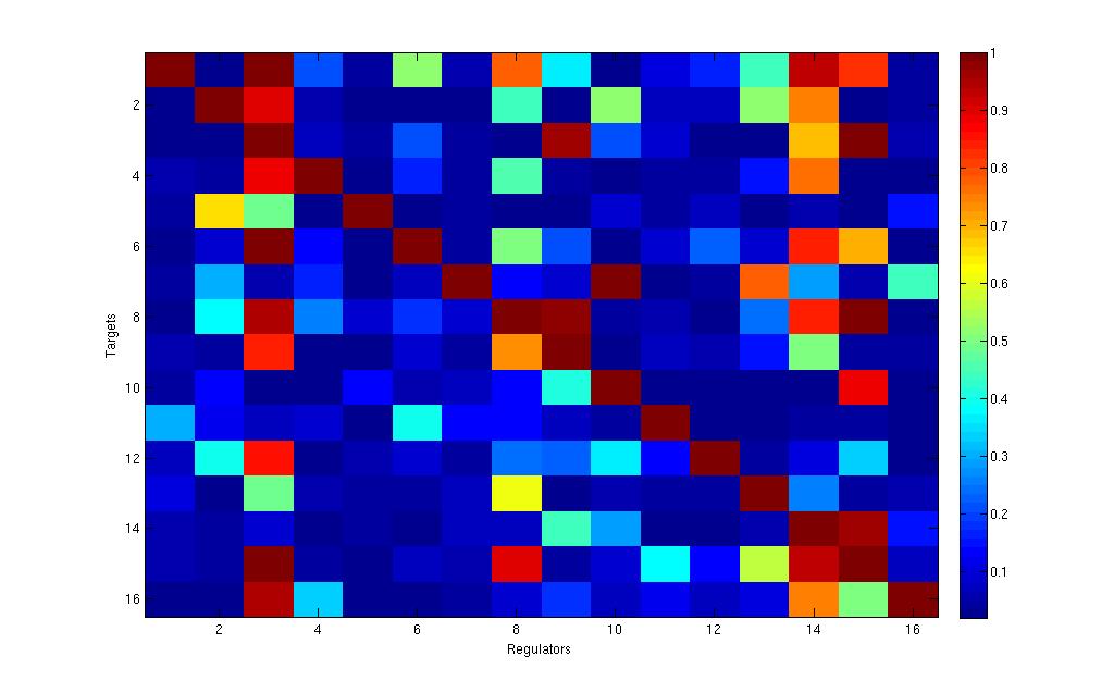
Figure 8. Heat-map representing the expected value for $p\left(\mathbf{H}|\centerdot\right)$ obtained by averaging the last 1000 samples. Rows represent targets and columns regulators. The diagonal indicates the decay parameters $\lambda$.

Appendix B Heatmaps and PR curves for the experiments

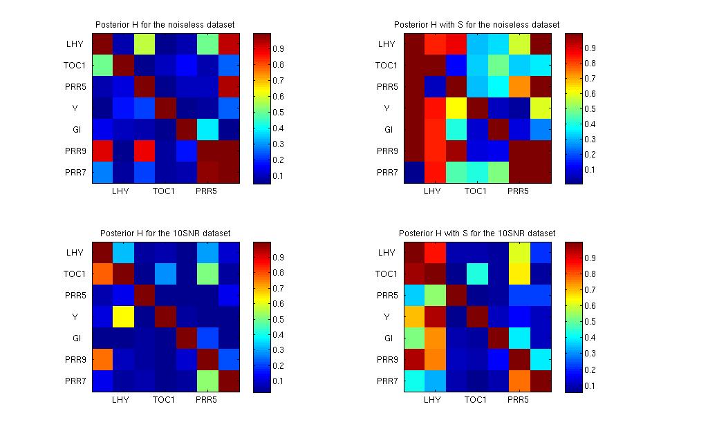
Figure 9. Heatmaps representing the posterior probability for the A. thaliana circadian clock network

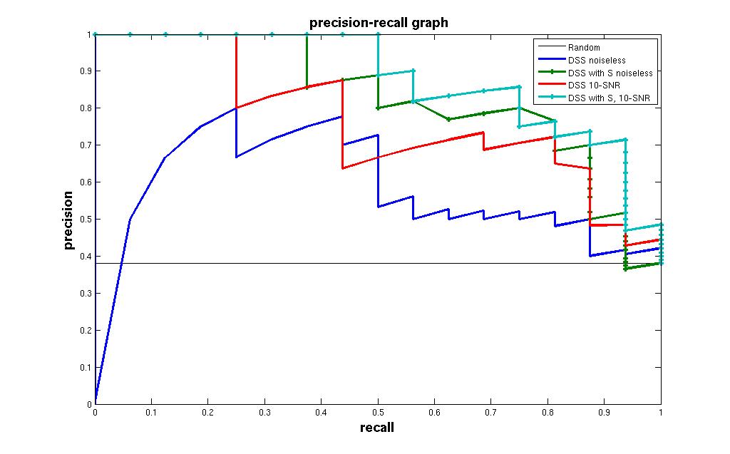
Figure 10. PR curves for the A. thaliana circadian clock network

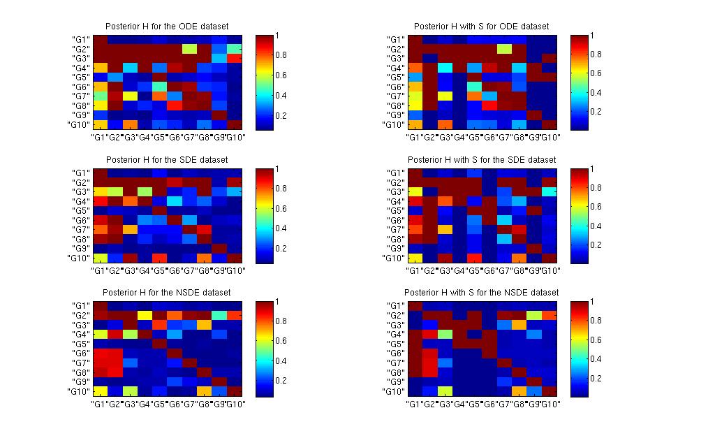
Figure 11. Heatmaps representing the posterior probability for the Dream4 Challenge network

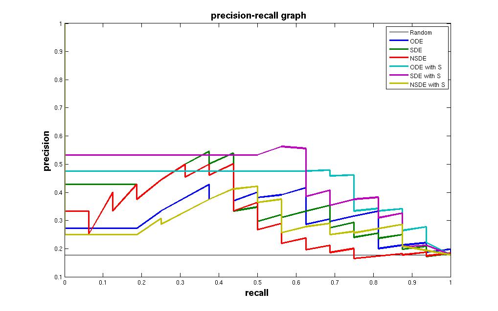
Figure 12. PR curves for the DREAM4 challenge network

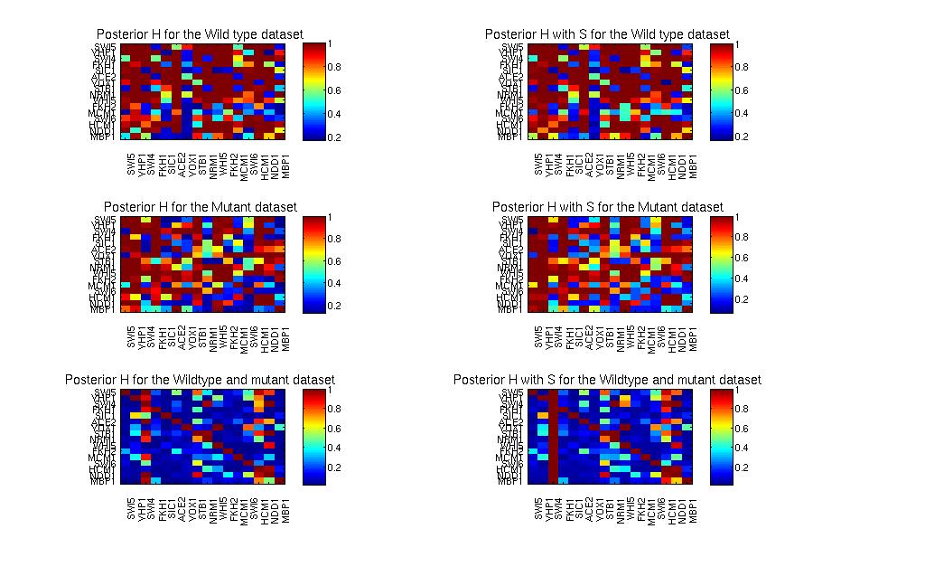
Figure 13. Heatmaps representing the posterior probability for the s. cerevisiae network

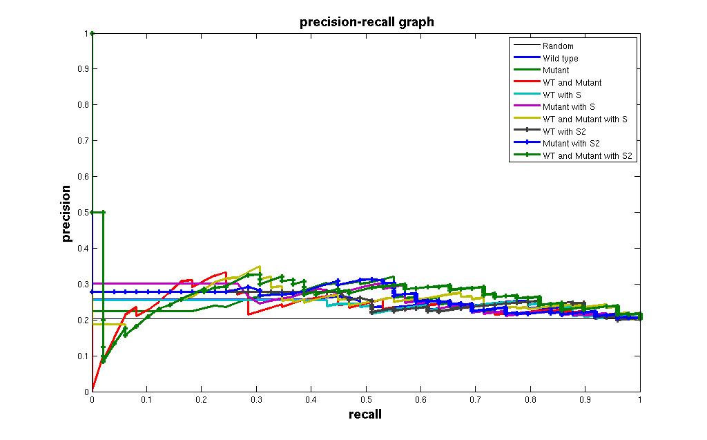
Figure 14. PR curves for the s. cerevisiae network

Appendix C A. thaliana circadian clock

The arabidopsis thaliana circadian clock model as presented in, is shown in Fig. 15.

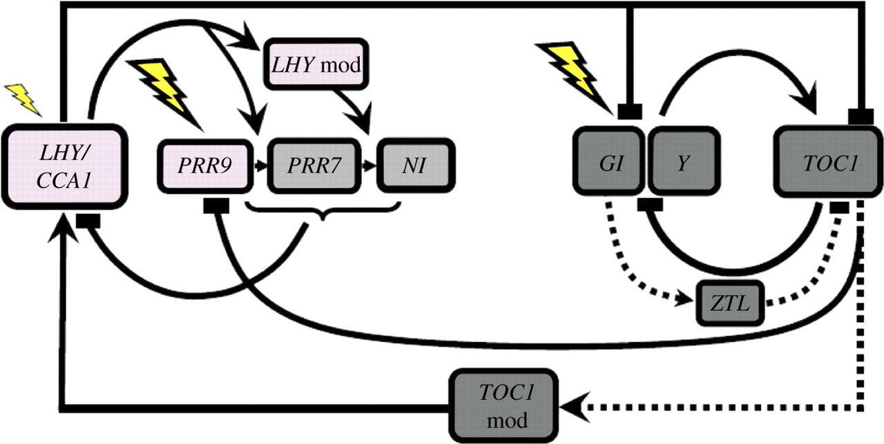
Figure 15. A. thaliana circadian clock model, transcriptional elements LHY, PRR9, PRR7, NI, Y, and TOC1. Post-transcriptional elements ZTL, TOC1mod and LHYmod. Light input is represented by a lighting symbol. Activating interactions are represented by solid line with arrows, repression by solid line with rectangles at the end, post transcriptional interactions are represented by dashed lines. .

Appendix D DREAM4 network

The 10-node oscillatory network that was part of the DREAM4 challenge supplementary information data set is presented in Fig. 16.

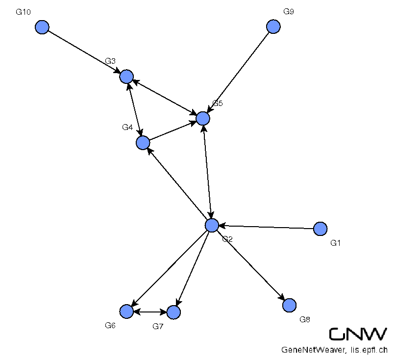
Figure 16. DREAM4 challenge network with 10 nodes, of those 3 are inputs, node G9 was subjected to a perturbation for half the time points.

Appendix E S. cerevisae cell cycle network

In Fig. 17 the inferred networks after thresholding the value of $p\left(h_{ij}=1\right)$ are presented, the putative ground truth matrix is presented on Fig. 18

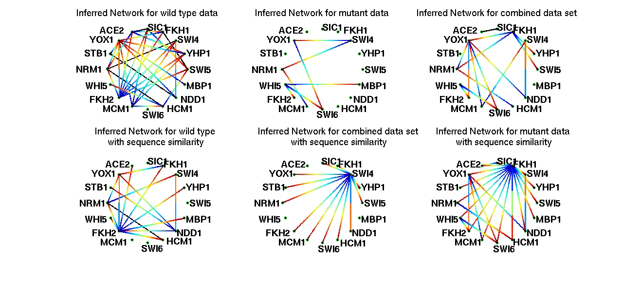
Figure 17. Inferred yeast networks for different data subsets with and without sequence information, edges go from blue (regulators) to red (targets)..

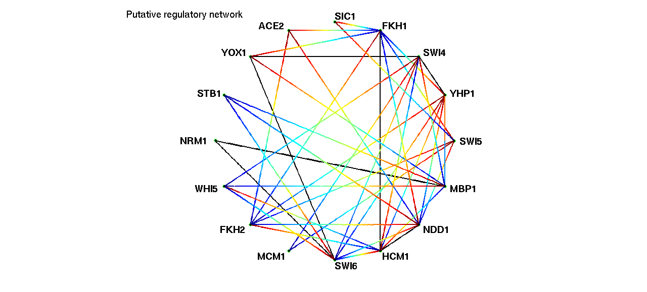
Figure 18. Putative yeast regulatory network edges go from blue (regulators) to red (targets)..

The putative regulatory network was built based on these references.

• Regulation of SIC1 by SWI5 as in [Weiss, 2012].

• Regulation of SWI4 by YHP1 as in [Bahler, 2005].

• Regulation of YHP1, SWI4, YOX1 and HCM1 by SWI4 as in [Macisaac et al, 2006].

• Regulation of SWI5 and ACE2 [Haase et al, 2014]; YHP1 [Macisaac et al, 2006]; SIC1, YOX1 and HCM1 [Venters et al, 2011]; NDD1 [Ostrow et al, 2014]; by FKH1.

• Regulation of SWI6 and MBP1 by NRM1 as in [Macisaac et al, 2006].

• Regulation of SWI6, SWI4 and MBP1 by WHI5 as in [Haase et al, 2014].

• Regulation of SWI5, YHP1 and FKH1 [Macisaac et al, 2006]; ACE2 and NDD1 [Haase et al, 2014] by FKH2.

• Regulation of SWI4 and SWI5 by MCM1 as in [Macisaac et al, 2006].

• Regulation of SWI4, FKH1, YOX1, NRM1, HCM1 and NDD1 as in [Macisaac et al, 2006].

• Regulation of YHP1, FKH1, FKH2, WHI5 and NDD1 by HCM1 as in [Pramila et al, 2006].

• Regulation of SWI5 and ACE2 [Haase et al, 2014]; YHP1 and HCM1 as in [Macisaac et al, 2006].

• Regulation of YHP1, FKH1, YOX1, NRM1 and HCM1 by MBP1 as in [Macisaac et al, 2006].

• Regulation of NDD1 [Macisaac et al, 2006]; SWI6 and MBP1 by the interaction of transcription factor MBF with STB1 [Stillman, 2013].

• Regulation of SWI4 and SWI6 by its cobinding with MCM1p as in [Haase et al, 2014].

References

- [Bell et al., 2005] Bell et al. (2005), Circadian rhythms from multiple oscillators: lessons from diverse organisms, Nature Review Genetics, 7, 544.
- [Bergersen et al., 2011] Bergersen et al. 2011, Weighted lasso with data integration,Statistical Applications in Genetics and Molecular Biology,10(1),1–29.
- [Bonham et al., 2013] Bonham et al. (2013), Alignment-free genetic sequence comparisons: a review of recent approaches by word analysis (2013), Briefings in Bioinformatics.
- [Bonneau et al., 2006] Bonneau et al. (2006), The inferelator: an algorithm for learning parsimonious regulatory networks from systems-biology data sets de novo,Genome biology, 7(5), R36.
- [Charbonnier et al., 2010] Charbonnier et al. (2010), Weighted-LASSO for structured network inference from time course data, Statistical applications in genetics and molecular biology, 9(1), 15.
- [Chen et al., 2004] Chen et al. (2004), Integrative analysis of cell cycle control in budding yeast,Molecular biology of the cell, 15(8),3841-3862.
- [Dalchau, 2011] Understanding biological timing using mechanistic and black-box models, New Phytologist.
- [DeJesus et al., 2013] DeJesus et al. (2013), A hidden markov model for identifying essential and growth-defect regions in bacterial genomes from transposon insertion sequencing data,BMC Bioinformatics, 14(1), 303.
- [Dondelinger et al., 2012] Dondelinger et al. (2012), Dynamic Bayesian networks in molecular plant science: inferring gene regulatory networks from multiple gene expression time series. Euphytica, 183 (3). pp. 361-377.
- [Dondelinger et al., 2013] Dondelinger et al. (2013), ODE parameter inference using adaptive gradient matching with Gaussian processes, In: Sixteenth International Conference on Artificial Intelligence and Statistics 29 Apr - 1 May 2013, Scottsdale, AZ, USA.
- [Edwards et al., 2010] Edwards et al. (2010), Quantitative analysis of regulatory flexibility under changing environmental conditions, Mol Syst Biol. 6: 425
- [Faith et al., 2007] Faith et al. (2007), Large-Scale Mapping and Validation of Escherichia coli Transcriptional Regulation from a Compendium of Expression Profiles, PLoS Biol, 5(1) e9.
- [Greenfield et al., 2013] Greenfield et al. (2013), Robust data-driven incorporation of prior knowledge into the inference of dynamic regulatory networks, Bioinformatics, 29(8),1060–1067.
- [Haase et al., 2014] Haase et al. (2014), Topology and control of the cell-cycle-regulated transcriptional circuitry, Genetics, 196(1),65–90.
- [Haury et al., 2012] Haury et al. (2012),TIGRESS: trustful inference of gene regulation using stability selection, BMC systems biology, 6(1),145.
- [Huynh-Thu et al., 2010] Huynh-Thu et al. (2010), Inferring regulatory networks from expression data using tree-based methods, PLoS ONE, 5(9), e12776.
- [Ishwaran et al., 2005] Ishwaran et al. (2005), Spike and slab variable selection: Frequentist and bayesian strategies, The Annals of Statistics, 33(2),730–773.
- [Kuffner et al., 2012] Kuffner et al. (2012),Inferring gene regulatory networks by ANOVA, Bioinformatics, 28(10), 1376–1382.
- [Kumar et al., 2000] Kumar et al.(2000), Forkhead transcription factors, fkh1p and fkh2p, collaborate with mcm1p to control transcription required for m-phase, Current Biology, 10(15), 896.
- [Li et al., 2006] Li et al (2006), Inferring regulatory networks using a hierarchical Bayesian graphical Gaussian model, Carnegie Mellon University, School of Computer Science, Machine Learning Department.
- [Li et al., 2004] Li et al. (2004), The yeast cell-cycle network is robustly designed. Proceedings of the National Academy of Sciences of the United States of America, 101(14), 4781.
- [Loy et al., 1999] Loy et al. (1999), NDD1, a high-dosage suppressor ofcdc28-1n, is essential for expression of a subset of late-s-phase-specific genes in saccharomyces cerevisiae,Molecular and cellular biology, 19(5), 3312.
- [Marbach et al, 2010] Marbach et al (2010), Revealing strengths and weaknesses of methods for gene network inference, PNAS 107(14), 6286–6291
- [Margolin et al., 2006] Margolin et al. (2006), ARACNE: An algorithm for the reconstruction of gene regulatory networks in a mammalian cellular context.BMC Bioinformatics, 7(Suppl 1), S7.
- [McClung, 2011] McClung (2011), Chapter 4 - the genetics of plant clocks, In Stuart Brody, editor, Advances in Genetics, volume Volume 74, pages 105–139. Academic Press.
- [Mirkin, 1987] Mirkin (1987), Additive clustering and qualitative factor analysis methods for similarity matrices, Journal of Classification, 4(1),7.
- [Morrissey et al., 2011] Morrisseyet al. (2011) Inferring the time-invariant topology of a nonlinear sparse gene regulatory network using fully Bayesian spline autoregression.Biostatistics, 12(4). pp. 682-694.
- [Oates et al., 2012] Oates et al. (2012), Network inference and biological dynamics. The Annals of Applied Statistics 6(3), 1209–1235.
- [Orlando et al., 2008] Orlando et al. (2008), Global control of cell-cycle transcription by coupled CDK and network oscillators, Nature, 453(7197), 944, June 2008.
- [Pokhilko et al., 2010] Pokhilko et al. (2010), Data assimilation constrains new connections and components in a complex, eukaryotic circadian clock model, Molecular Systems Biology, 6.
- [Pokhilko et al., 2012] Pokhilko et al. (2012), The clock gene circuit in arabidopsis includes a repressilator with additional feedback loops,Molecular Systems Biology, 8.
- [Pramila, 2006] Pramila (2006), The forkhead transcription factor hcm1 regulates chromosome segregation genes and fills the s-phase gap in the transcriptional circuitry of the cell cycle,Genes & Development, 20(16), 2266.
- [Sievers et al., 2011] Sievers et al. (2011), Fast, scalable generation of high-quality protein multiple sequence alignments using Clustal Omega, Molecular Systems Biology, 7(1).
- [Sims et al., 2009] Sims et al. (2009), Alignment-free genome comparison with feature frequency profiles (FFP) and optimal resolutions. Proceedings of the National Academy of Sciences of the United States of America, 106(8), 2677–2682.
- [Spellman, 1998] Spellman (1998), Comprehensive identification of cell cycle regulated genes of the yeast saccharomyces cerevisiae by microarray hybridization,Molecular biology of the cell, 9(12), 3273.
- [Tibshirani, 1994] Tibshirani (1994), Regression shrinkage and selection via the lasso. volume 58, pages 267, 1994.
- [Turner, 2012] Turner (2012) Cell size control in yeast. Current Biology, 22(9), R350.
- [Venters, 2011] Venters (2011), A comprehensive genomic binding map of gene and chromatin regulatory proteins in saccharomyces, Molecular Cell, 41(4), 480.
- [Zhu et al., 1999] Zhu et al. (1999), SCPD: a promoter database of the yeast Saccharomyces cerevisiae.Bioinformatics, 15(7), 607.

References

- [Bahler, 2005] Bahler (2005), Cell-cycle control of gene expression in budding and fission yeast. Annu Rev Genet, 39 69–94.
- [Haase et al, 2014] Haase et al (2014),Topology and control of the cell-cycle-regulated transcriptional circuitry, Genetics, 196(1), 65–90.
- [Ishwaran et al., 2005] Ishwaran et al. (2005), Spike and slab variable selection: Frequentist and bayesian strategies, The Annals of Statistics, 33(2),730–773.
- [Macisaac et al, 2006] Macisaac et al (2006), An improved map of conserved regulatory sites for Saccharomyces cerevisiae, BMC Bioinformatics, 7(113).
- [Marbach et al, 2010] Marbach et al (2010), Revealing strengths and weaknesses of methods for gene network inference, PNAS 107(14), 6286–6291
- [Ostrow et al, 2014] Ostrow et al (2014),Fkh1 and Fkh2 Bind Multiple Chromosomal Elements in the S. cerevisiae Genome with Distinct Specificities and Cell Cycle Dynamics, PLoS ONE 9(2).
- [Pokhilko et al., 2010] Pokhilko et al. (2010), Data assimilation constrains new connections and components in a complex, eukaryotic circadian clock model, Molecular Systems Biology, 6.
- [Pramila et al, 2006] Pramila et al (2006),The Forkhead transcription factor Hcm1 regulates chromosome segregation genes and fills the S-phase gap in the transcriptional circuitry of the cell cycle, Genes Dev, 20(16), 2266–78.
- [Stillman, 2013] Stillman (2013),Dancing the cell cycle two-step: regulation of yeast G1-cell-cycle genes by chromatin structure, Trends Biochem Sci, 38(9), 467–75.
- [Venters et al, 2011] Venters et al (2011), A comprehensive genomic binding map of gene and chromatin regulatory proteins in Saccharomyces, Mol Cell, 41(4), 480–92.
- [Weiss, 2012] Weiss (2012), YeastBook - Cell Signaling and Development: Mitotic Exit and Separation of Mother and Daughter Cells, Genetics 192, 1165–1202;