Harmonic and Subharmonic Association and Dissociation
of Universal Dimers in a Thermal Gas

Abstract

In a gas of ultracold atoms whose scattering length is controlled by a magnetic Feshbach resonance, atoms can be associated into universal dimers by an oscillating magnetic field. In addition to the harmonic resonance with frequency near that determined by the dimer binding energy, there is a subharmonic resonance with half that frequency. If the thermal gas contains dimers, they can be dissociated into unbound atoms by the oscillating magnetic field. We show that the transition rates for association and dissociation can be calculated by treating the oscillating magnetic field as a sinusoidal time-dependent perturbation proportional to the contact operator. Many-body effects are taken into account through transition matrix elements of the contact operator. We calculate both the harmonic and subharmonic transition rates analytically for association in a thermal gas of atoms and dissociation in a thermal gas of dimers.

I Introduction

The use of magnetic Feshbach resonances to control the interaction strengths of ultracold atoms has led to significant advances in our understanding of strong interactions in few-body and many-body physics. The effects of time-dependent strong interactions can be studied by using a time-dependent magnetic field. A particularly interesting case is a sinusoidally modulated magnetic field. Atoms can be associated into universal molecules composed of atoms with a large scattering length by modulating the magnetic field with a frequency near that determined by the binding energy of the molecule. The measurement of the binding energy of a molecule by the resonance in the oscillation frequency is called magnetic-field modulation spectroscopy or sometimes wiggle spectroscopy.

Modulation of the magnetic field was pioneered by Thompson, Hodby, and Wieman to associate ⁸⁵Rb atoms into dimers Wieman0505 . Papp and Wieman used magnetic-field modulation spectroscopy to measure the small binding energies of dimers composed of ⁸⁵Rb and ⁸⁷Rb atoms Wieman0607 . Weber et al. used a resonantly modulated magnetic field to associate ⁴¹K and ⁸⁷Rb atoms into dimers and to measure their binding energies Inguscio0808 . They also observed subharmonic resonances at half the frequency determined by the binding energies of the dimers. Lange et al. used magnetic-field modulation spectroscopy to measure the binding energies of ¹³³Cs dimers Grimm0810 . Pollack et al. used a modulated magnetic field to excite collective modes in a Bose-Einstein condensate of ⁷Li atoms Hulet1004 . Machtey et al.  used a modulated magnetic field to associate ⁷Li atoms into Efimov trimers Khaykovich1201 . Dyke, Pollack, and Hulet used magnetic-field modulation spectroscopy to measure the binding energies of ⁷Li dimers in both a Bose-Einstein condensate and a thermal gas Hulet1302 . In the thermal gas, they also observed a subharmonic resonance. Smith recently pointed out that a sinusoidally oscillating magnetic field near a Feshbach resonance can also be used to control the scattering length, and he showed that the resonance parameters are universal functions of the magnetic field DHSmith1503 .

A theoretical treatment of the association of atoms into dimers by an oscillating magnetic field was first presented by Hanna, Köhler, and Burnett in 2007 HKB0609 . An alternative approach was recently developed by Brouard and Plata BP1503 . Both groups described the two-atom system by a two-channel model consisting of a continuum of atom-pair states and a discrete molecular state. They calculated the probability for the association of atom pairs into dimers as a function of time by solving the time-dependent Schrödinger equation for the two coupled channels. In Ref. BP1503 , some qualitative aspects of the harmonic and subharmonic association processes were derived analytically. The results for association probabilities from both groups were completely numerical.

A much simpler approach to this problem was recently introduced in Ref. LSB:1406 . It was inspired by Tan’s adiabatic relation, which expresses the change in the energy $E$ of a system due to a change in the scattering length $a$ in terms of an extensive thermodynamic variable that is conjugate to $1/a$ called the contact $C$ Tan0508 . In the case of fermions with mass $m$ and two spin states, the adiabatic relation is

$$\frac{d~{}~{}~{}}{d(1/a)}E=-\frac{\hbar^{2}}{4\pi m}C.$$ (1)

(In the case of identical bosons, the right side should be multiplied by $1/2$.) Ref. LSB:1406 pointed out that the transition rates for the association of atoms into universal dimers can be calculated by treating the oscillating magnetic field as a sinusoidal time-dependent perturbation proportional to the contact operator. The association rates were calculated for a thermal gas of atoms and for a dilute Bose-Einstein condensate of atoms. In this approach, many-body effects are taken into account through transition matrix elements of the contact operator.

In this paper, we extend the approach of Ref. LSB:1406 to the dissociation rates of universal dimers and to subharmonic transitions. In Sections II, we derive general formulas for the harmonic and subharmonic transition rates using time-dependent perturbation theory. In Sections III and IV, we calculate the leading harmonic contributions to the association rate in a thermal gas of atoms and the dissociation rate in a thermal gas of dimers. They come from a first-order perturbation in the contact operator. In Sections V and VI, we calculate the dominant subharmonic contributions to the association rate in a thermal gas of atoms and the dissociation rate in a thermal gas of dimers. They come from a second-order perturbation in the contact operator. In Section VII, we apply our results for the association rate to a thermal gas of ⁷Li atoms. In Section VIII, we summarize previous theoretical treatments of association into dimers using a modulated magnetic field, and we compare them with our results for association.

II Transition Rates

In this section, we derive general formulas for transition rates at first order and second order in time-dependent perturbation theory. We focus on the case of fermionic atoms with equal mass $m$ and two spin states. (We also give the corresponding results for identical bosons.)

II.1 Perturbing Hamiltonians

Near a magnetic Feshbach resonance, the scattering length $a$ of the atoms is a function of the magnetic field:

$$a(B)=a_{\rm bg}[1-\Delta/(B-B_{0})],$$ (2)

where $a_{\rm bg}$ is the background scattering length and $B_{0}$ and $B_{0}+\Delta$ are the positions of the pole and the zero of the scattering length, respectively. We consider a time-dependent magnetic field that has a constant value $\bar{B}$ for $t<0$ and is modulated with a small amplitude $b$ around the average value $\bar{B}$ for $t>0$:

$$B(t) = \bar{B}\hskip 85.35826ptt<0,$$ (3)

$$= \bar{B}+b\sin(\omega t)\hskip 28.45274ptt>0.$$

If the oscillating magnetic field is inserted into Eq. (2), it implies a time-dependent scattering length $a(t)$.

Tan’s adiabatic relation in Eq. (1) implies that the leading perturbation in the Hamiltonian for $t>0$ is proportional to the contact operator:

$$H(t)-H(0)=-\frac{\hbar^{2}}{4\pi m}\left(\frac{1}{a(t)}-\frac{1}{\bar{a}}\right)C,$$ (4)

where $\bar{a}=a(\bar{B})$ is the scattering length in the absence of the modulated magnetic field. In Appendix A, quantum field theory methods are used to argue that this is the only perturbation that contributes in the zero-range limit. The inverse scattering length can be expanded in powers of $b$:

$$\frac{1}{a(t)}=\frac{1}{\bar{a}}-\frac{1}{a_{\rm bg}}\left(\frac{b\Delta}{(\Delta+B_{0}-\bar{B})^{2}}\right)\sin(\omega t)-\frac{1}{a_{\rm bg}}\left(\frac{b^{2}\Delta}{(\Delta+B_{0}-\bar{B})^{3}}\right)\sin^{2}(\omega t)+\ldots.$$ (5)

The coefficients of the powers of $b$ have well-behaved limits as $\bar{B}$ approaches the Feshbach resonance at $B_{0}$. Inserting the expansion in Eq. (5) into Eq. (4), we can identify terms in the perturbing Hamiltonian that are first and second order in $b$:

$$H_{\rm 1}(t) = \frac{\hbar^{2}}{4\pi ma_{\rm bg}}\left(\frac{b\Delta}{(\Delta+B_{0}-\bar{B})^{2}}\right)C\sin(\omega t),$$ (6a)

$$H_{\rm 2}(t) = \frac{\hbar^{2}}{4\pi ma_{\rm bg}}\left(\frac{b^{2}\Delta}{(\Delta+B_{0}-\bar{B})^{3}}\right)C\sin^{2}(\omega t).$$ (6b)

(In the case of identical bosons, the right sides should be multiplied by $1/2$.) If $|b|\ll|\Delta|$, the effects of $H_{1}$ and $H_{2}$ can be taken into account as time-dependent perturbations. The first-order perturbation in $H_{\rm 1}$ drives transitions to states whose energies are higher or lower by $\hbar\omega$. We refer to such transitions as harmonic transitions. The first-order perturbation in $H_{\rm 2}$ and the second-order perturbation in $H_{\rm 1}$ both drive transitions to states whose energies differ by 0 or $\pm 2\hbar\omega$. We refer to transitions to states whose energies are higher or lower by $2\hbar\omega$ as subharmonic transitions.

II.2 Fermi’s Golden Rule

We first consider transitions from the first-order perturbation in $H_{\rm 1}$. We take the initial state $|i\rangle$ to be an energy eigenstate with energy $E_{i}$. We consider the transition to a distinct energy eigenstate $|f\rangle$ with energy $E_{f}$. At first order in perturbation theory, the probability amplitude for the final state $|f\rangle$ at time $T$ is

$$a_{f}^{(1)}(T)=\frac{i\hbar}{8\pi ma_{\rm bg}}\left(\frac{b\Delta}{(\Delta+B_{0}-\bar{B})^{2}}\right)\left[\frac{e^{i(\omega_{fi}+\omega)T}-1}{\omega_{fi}+\omega}-\frac{e^{i(\omega_{fi}-\omega)T}-1}{\omega_{fi}-\omega}\right]\langle f|C|i\rangle,$$ (7)

where $\omega_{fi}=(E_{f}-E_{i})/\hbar$. The two terms inside the brackets have absolute values that increase linearly with $T$ in the limits $\omega_{fi}\to-\omega$ and $\omega_{fi}\to+\omega$, respectively. By applying Fermi’s Golden Rule, we obtain the transition rate summed over final states $|f\rangle$:

$$\Gamma_{1}^{(1)}(\omega)=\frac{\hbar^{2}}{64\pi^{2}m^{2}a_{\rm bg}^{2}}\left(\frac{b\Delta}{(\Delta+B_{0}-\bar{B})^{2}}\right)^{2}\sum_{f}\big{|}\langle f|C|i\rangle\big{|}^{2}\sum_{\pm}2\pi\delta(\omega_{fi}\pm\omega).$$ (8)

(In the case of identical bosons, the prefactor should be multiplied by $1/4$.) This transition rate is non-zero only for final states whose energy differs from $E_{i}$ by $\pm\hbar\omega$, so it contributes to the harmonic transition rate $\Gamma_{1}(\omega)$. The superscript (1) on $\Gamma_{1}^{(1)}$ indicates that it comes from the first-order perturbation in $H_{1}$.

We next consider transitions from the first-order perturbation in $H_{2}$. At first order in perturbation theory, the probability amplitude for the final state $|f\rangle$ at time $T$ is

$$a_{f}^{(2)}(T)=\frac{\hbar}{16\pi ma_{\rm bg}}\left(\frac{b^{2}\Delta}{(\Delta+B_{0}-\bar{B})^{3}}\right)\left[\frac{e^{i(\omega_{fi}+2\omega)T}-1}{\omega_{fi}+2\omega}+\frac{e^{i(\omega_{fi}-2\omega)T}-1}{\omega_{fi}-2\omega}+\ldots\right]\langle f|C|i\rangle.$$ (9)

Inside the brackets, we have shown explicitly only those terms whose absolute values increase linearly with $T$ in the limits $\omega_{fi}\to\pm 2\omega$. By applying Fermi’s Golden Rule, we obtain the transition rate summed over final states $|f\rangle$:

$$\Gamma_{2}^{(2)}(\omega)=\frac{\hbar^{2}}{256\pi^{2}m^{2}a_{\rm bg}^{2}}\left(\frac{b^{2}\Delta}{(\Delta+B_{0}-\bar{B})^{3}}\right)^{2}\sum_{f}\big{|}\langle f|C|i\rangle\big{|}^{2}\sum_{\pm}2\pi\delta(\omega_{fi}\pm 2\omega).$$ (10)

(In the case of identical bosons, the prefactor should be multiplied by $1/4$.) This transition rate is nonzero only for final states whose energy differs from $E_{i}$ by $\pm 2\hbar\omega$, so it contributes to the subharmonic transition rate $\Gamma_{2}(\omega)$. The superscript (2) on $\Gamma_{2}^{(2)}$ indicates that it comes from the first-order perturbation in $H_{2}$. The subharmonic transition rate in Eq. (10) is determined by the same transition matrix element $\langle f|C|i\rangle$ of the contact operator as the harmonic transition rate in Eq. (8). It can be expressed in terms of the leading harmonic transition rate at twice the frequency:

$$\Gamma_{2}^{(2)}(\omega)=\frac{1}{4}\left(\frac{b}{\Delta+B_{0}-\bar{B}}\right)^{2}\Gamma_{1}^{(1)}(2\omega).$$ (11)

Finally we consider transitions from the second-order perturbation in $H_{\rm 1}$. At second order in perturbation theory, the probability amplitude for the final state $|f\rangle$ at time $T$ is

$$a_{f}^{(1,1)}(T) = -\frac{\hbar^{2}}{64\pi^{2}m^{2}a_{\rm bg}^{2}}\left(\frac{b\Delta}{(\Delta+B_{0}-\bar{B})^{2}}\right)^{2}\sum_{m\neq i}\langle f|C|m\rangle\langle m|C|i\rangle$$ (12)

$$\hskip 71.13188pt\times\left[\frac{e^{i(\omega_{fi}+2\omega)T}-1}{(\omega_{fi}+2\omega)(\omega_{mi}+\omega)}+\frac{e^{i(\omega_{fi}-2\omega)T}-1}{(\omega_{fi}-2\omega)(\omega_{mi}-\omega)}+\ldots\right],$$

where the sum is over intermediate states $|m\rangle$ distinct from $|i\rangle$. Inside the brackets, we have shown explicitly only those terms whose absolute values increase linearly with $T$ if $\omega_{fi}$ is $\pm 2\omega$. By applying Fermi’s Golden Rule, we obtain the transition rate summed over final states $|f\rangle$:

$$\Gamma_{2}^{(1,1)}(\omega)=\frac{\hbar^{4}}{4096\pi^{4}m^{4}a_{\rm bg}^{4}}\left(\frac{b\Delta}{(\Delta+B_{0}-\bar{B})^{2}}\right)^{4}\sum_{f}\sum_{\pm}\left|\sum_{m\neq i}\frac{\langle f|C|m\rangle\langle m|C|i\rangle}{\omega_{mi}\pm\omega}\right|^{2}2\pi\delta(\omega_{fi}\pm 2\omega).$$ (13)

(In the case of identical bosons, the prefactor should be multiplied by 1/16.) This transition rate is nonzero only for final states whose energy differs from $E_{i}$ by $\pm 2\hbar\omega$, so it contributes to the subharmonic transition rate $\Gamma_{2}(\omega)$. The superscript (1,1) on $\Gamma_{2}^{(1,1)}$ indicates that it comes from the second-order perturbation in $H_{1}$. There is an additional factor of $1/a_{\rm bg}^{2}$ in the prefactor for $\Gamma_{2}^{(1,1)}$ compared to $\Gamma_{2}^{(2)}$. The relative importance of these two contributions is determined by the canceling length scales provided by the contact matrix elements and the frequency denominator. If $\Gamma_{2}^{(1,1)}$ and $\Gamma_{2}^{(2)}$ have the same order of magnitude, the interference between the first-order perturbation in $H_{2}$ and the second-order perturbation in $H_{1}$ would have to be taken into account. By explicit calculations of subharmonic transition rates in a thermal gas, we will find that the additional dimensionless factor in $\Gamma_{2}^{(1,1)}$ is $(\bar{a}/a_{\rm bg})^{2}$. Thus $\Gamma_{2}^{(1,1)}$ is much larger than $\Gamma_{2}^{(2)}$ if $\bar{B}$ is near a Feshbach resonance.

II.3 Thermal System

The transitions rates in Eqs. (8), (10), and (13) apply to an initial state $|i\rangle$ that is an energy eigenstate. A thermal system is described instead by a density matrix. For a completely thermalized system, the density matrix is $\rho=\exp(-\beta H)/{\rm Tr}(\exp(-\beta H))$, where $H$ is the Hamiltonian and $\beta=1/k_{B}T$. By expressing the modulus-squared of an amplitude as the product of the amplitude and its complex conjugate, the dependence on the initial state in Eqs. (8), (10), and (13) can be put in the form of the projection operator $|i\rangle\langle i|$ multiplied by a function $F(E_{i})$ of the initial energy that includes the frequency delta function. If the density matrix $\rho$ is diagonal in an energy basis, the transition rate is obtained by making the substitution

$$F(E_{i})\,|i\rangle\langle i|\longrightarrow\sum_{i}F(E_{i})\,|i\rangle\langle i|\rho|i\rangle\langle i|.$$ (14)

II.4 Homogeneous System

The contact operator $C$ is an extensive variable. It can be expressed as the integral over space of the contact density operator:

$$C=\int d^{3}r\,{\cal C}(\bm{r}).$$ (15)

If the initial and final states are homogeneous systems, we can simplify the transition rates by expressing them in terms of matrix elements of the contact density operator.

The harmonic transition rate $\Gamma_{1}^{(1)}(\omega)$ in Eq. (8) and the subharmonic transition rate $\Gamma_{2}^{(2)}(\omega)$ in Eq. (10) involve the factor $|\langle f|C|i\rangle|^{2}$. By inserting the expression for $C$ in Eq. (15), we obtain matrix elements of the contact density at two different positions. We can use translational invariance to put both operators at the same position $\bm{r}$. One of the integrals over space then gives a momentum-conserving delta function. The resulting expression for the modulus-squared of the transition matrix element is

$$\sum_{f}\big{|}\langle f|C|i\rangle\big{|}^{2}=\sum_{f}(2\pi)^{3}\delta^{3}(\bm{K}_{f}-\bm{K}_{i})\int\!d^{3}r\,\big{|}\langle f|{\cal C}(\bm{r})|i\rangle\big{|}^{2},$$ (16)

where $\bm{K}_{i}$ and $\bm{K}_{f}$ are the total wave vectors of the initial and final states of the homogeneous system, respectively. Homogeneity implies that $\big{|}\langle f|{\cal C}(\bm{r})|i\rangle\big{|}^{2}$ is independent of the position $\bm{r}$. Thus the integral $\int\!d^{3}r$ in Eq. (16) just gives a factor of the volume $V$.

The subharmonic transition rate $\Gamma_{2}^{(1,1)}(\omega)$ in Eq. (13) involves the product of four matrix elements of $C$. By inserting the expression for $C$ in Eq. (15), we obtain matrix elements of the contact density at four different positions. We can use translational invariance to put all four operators at the same position $\bm{r}$. Three of the integrals over space then give momentum-conserving delta functions. The resulting expression for the factor in Eq. (13) that involves matrix elements of $C$ is

$$\sum_{f}\left|\sum_{m\neq i}\frac{\langle f|C|m\rangle\langle m|C|i\rangle}{\omega_{mi}\pm\omega}\right|^{2} = \sum_{f}(2\pi)^{3}\delta^{3}(\bm{K}_{f}-\bm{K}_{i})\int d^{3}r$$ (17)

$$\times\sum_{m\neq i}(2\pi)^{3}\delta^{3}(\bm{K}_{m}-\bm{K}_{i})\ \frac{\langle f|{\cal C}(\bm{r})|m\rangle\langle m|{\cal C}(\bm{r})|i\rangle}{\omega_{mi}\pm\omega}\,$$

$$\times\sum_{m^{\prime}\neq i}(2\pi)^{3}\delta^{3}(\bm{K}_{m^{\prime}}-\bm{K}_{i})\frac{\langle i|{\cal C}(\bm{r})|m^{\prime}\rangle\langle m^{\prime}|{\cal C}(\bm{r})|f\rangle}{\omega_{m^{\prime}i}\pm\omega},$$

where $\bm{K}_{m}$ and $\bm{K}_{m^{\prime}}$ are the total momenta of the intermediate states $|m\rangle$ and $|m^{\prime}\rangle$, respectively. Homogeneity implies that the integrand is independent of the position $\bm{r}$. Thus the integral $\int\!d^{3}r$ just gives a factor of the volume $V$.

II.5 Local Density Approximation

For a many-body system whose number density varies slowly with the position $\bm{r}$, the transition rate can be simplified by using the local density approximation. The transition rate is an extensive quantity. For a homogeneous system, the expressions obtained by inserting Eq. (16) or Eq. (17) into the transition rate have an explicit factor of the volume $\int d^{3}r=V$. If the transition rate is also proportional to the total number $N_{i}$ of some type of particle, the additional factor must be the intensive combination $N_{i}/V$. For a homogeneous system consisting of fermionic atoms with spin states 1 and 2, the association rate is proportional to $N_{1}N_{2}$. The local density approximation for the association rate in a system with local number densities $n_{1}(\bm{r})$ and $n_{2}(\bm{r})$ can be obtained by making the substitution

$$N_{1}N_{2}/V\longrightarrow\int d^{3}r\,n_{1}(\bm{r})n_{2}(\bm{r}).$$ (18)

For a homogeneous system consisting of dimers, the disssociation rate is proportional to their total number $N_{\rm D}$. The local density approximation for the disssociation rate in a system with local number density $n_{\rm D}(\bm{r})$ can be obtained by making the substitution

$$N_{\rm D}\longrightarrow\int d^{3}r\,n_{\rm D}(\bm{r}).$$ (19)

III Harmonic Association Rate

A pair of atoms with a large positive scattering length can be associated into a universal dimer by an oscillating magnetic field. In this section, we calculate the harmonic association rate in a thermal gas of atoms. We also give the subharmonic association rate from first-order perturbation theory. We consider a gas of atoms that is in thermal equilibrium at temperature $T$. For simplicity, we take the number densities $n_{1}$ and $n_{2}$ of the atoms to be sufficiently low that their distributions are given by Boltzmann statistics instead of Fermi-Dirac statistics.

III.1 Initial and Final States

We first consider a homogeneous gas consisting of $N_{1}$ atoms of spin state 1 and $N_{2}$ atoms of spin state 2 in a volume $V$. The two spin states interact with a large positive scattering length $\bar{a}$. The universal dimer has a small binding energy $\hbar^{2}/m\bar{a}^{2}$. For a gas in thermal equilibrium, the harmonic transition rate is given by Eq. (8) with the substitution in Eq. (14), where $\rho=\rho_{\rm gas}$ is the density matrix for the thermal gas of atoms. To simplify the presentation, we will temporarily ignore the frequency delta function, which depends on the energy $E_{i}$ of the states in the density matrix. The terms in Eq. (8) that depend on the contact operator can then be expressed compactly as $\sum_{f}\langle f|C\rho_{\rm gas}C|f\rangle$. We will insert the frequency delta function at the end of the calculation.

In the low-density limit where 3-body and higher-body correlations can be neglected, the density matrix $\rho_{\rm gas}$ can be expressed in terms of the density matrix $\rho_{\rm pair}$ for a pair of atoms in thermal equilibrium:

$$\sum_{f}\langle f|C\rho_{\rm gas}C|f\rangle=N_{1}N_{2}\sum_{f}\langle f|C\rho_{\rm pair}C|f\rangle.$$ (20)

The factor $N_{1}N_{2}$ is the number of pairs of fermions in the two spin states. (For a gas of $N$ identical bosons, the number of pairs is $N^{2}/2$.) The pair density matrix is normalized: Tr$(\rho_{\rm pair})=1$. On the left side of Eq. (20), the sum over $f$ is over many-body final states that include a single dimer. On the right side, the sum over $f$ is over two-atom final states that consist of a single dimer. The density matrix for a pair of atoms in thermal equilibrium is

$$\rho_{\rm pair}=\frac{\lambda_{\rm T}^{6}}{V^{2}}\int_{\bm{K}}\int_{\bm{k}}\exp(-\beta\hbar^{2}K^{2}/4m-\beta\hbar^{2}k^{2}/m)|\bm{K},\bm{k}\rangle\langle\bm{k},\bm{K}|,$$ (21)

where $\beta=1/k_{B}T$ and $\lambda_{\rm T}$ is the thermal deBroglie wavelength for an atom with mass $m$:

$$\lambda_{\rm T}=\sqrt{2\pi\hbar^{2}/mk_{\rm B}T}.$$ (22)

The two-atom states $|\bm{K},\bm{k}\rangle$ in Eq. (21) are labeled by the center-of-mass wave vector $\bm{K}=\bm{k}_{1}+\bm{k}_{2}$ and the relative wave vector $\bm{k}=(\bm{k}_{1}-\bm{k}_{2})/2$. The integrals over the wave vectors are defined by

$$\int_{\bm{k}}\equiv\int\frac{d^{3}k}{(2\pi)^{3}}.$$ (23)

The wave vector states have delta-function normalizations: $\langle\bm{k}^{\prime}|\bm{k}\rangle=(2\pi)^{3}\delta^{3}(\bm{k}^{\prime}-\bm{k})$. In the case $\bm{k}^{\prime}=\bm{k}$, the infinite norm can be expressed as a factor of the volume: $\langle\bm{k}|\bm{k}\rangle=V$. The energy of a pair of atoms in the state $|\bm{K},\bm{k}\rangle$ is

$$E_{\rm AA}=\hbar^{2}K^{2}/4m+\hbar^{2}k^{2}/m.$$ (24)

The sum over final states on the right hand side of Eq. (20) can be expressed as an integral over the wave vector ${\bm{k}}_{\rm D}$ of a dimer:

$$\sum_{f}\langle f|C\rho_{\rm pair}C|f\rangle=\int_{\bm{k}_{\rm{D}}}\langle{\bm{k}}_{\rm D}|C\rho_{\rm pair}C|{\bm{k}}_{\rm D}\rangle.$$ (25)

The energy of the dimer is

$$E_{\rm D}=-\hbar^{2}/m\bar{a}^{2}+\hbar^{2}k_{\rm D}^{2}/4m.$$ (26)

III.2 Matrix Elements

Because the system is homogeneous, the analog of Eq. (16) can be used to express the contact operators $C$ on the right side of Eq. (25) in terms of contact density operators at the same position $\bm{r}$. The wave vector delta function in Eq. (16) reduces to $\delta^{3}(\bm{k}_{\rm D}-\bm{K})$, and it can be used to integrate over $\bm{k}_{\rm D}$. The frequency delta function in Eq. (8) reduces to

$$\sum_{\pm}2\pi\delta\big{(}(E_{\rm D}-E_{\rm AA})/\hbar\pm\omega\big{)}=2\pi\delta\big{(}\omega-\hbar/m\bar{a}^{2}-\hbar k^{2}/m\big{)}.$$ (27)

In the sum over $\pm\omega$, only the $+\omega$ term contributes.

The expression for the transition rate has been reduced to matrix elements of the contact density operator of the form $\langle{\bm{k}}_{\rm D}|{\cal C}({\bm{r}})|{\bm{K}},{\bm{k}}\rangle$. The matrix element is calculated in Appendix B, and is given by Eq. (73):

$$\langle{\bm{k}}_{\rm D}|{\cal C}(\bm{r})|{\bm{K}},{\bm{k}}\rangle=\frac{\sqrt{128\pi^{3}\bar{a}}}{1-i\bar{a}k}.$$ (28)

The Gaussian integral over $\bm{K}$ can be evaluated analytically. The sum over final states of the matrix element in Eq. (25) reduces to

$$\sum_{f}\langle f|C\rho_{\rm gas}{C^{\dagger}}|f\rangle=128\sqrt{2}\pi\bar{a}\lambda_{\rm T}^{3}\frac{N_{1}N_{2}}{V}\int_{0}^{\infty}dk\frac{k^{2}}{1+k^{2}\bar{a}^{2}}\exp(-\beta\hbar^{2}k^{2}/m).$$ (29)

Before integrating over $k$, this must be multiplied by the frequency delta function in Eq. (27).

III.3 Harmonic Association Rate

Our final result for the harmonic association rate $\Gamma_{1}^{(1)}(\omega)$ in the homogeneous gas can be obtained from Eq. (8) by replacing $\sum_{f}|\langle f|C|i\rangle|^{2}$ by the right side of Eq. (29), replacing the sum of frequency delta functions by the right side of Eq. (27), and then using the delta function to integrate over $k$. The local density approximation can be implemented by making the substitution for $N_{1}N_{2}/V$ in Eq. (18). The threshold angular frequency for association is $\hbar/m\bar{a}^{2}$: the emission of a smaller energy from a pair of atoms is not enough to allow a transition to dimer. For $\omega>\hbar/m\bar{a}^{2}$, the harmonic association rate is

$$\Gamma_{1}^{(1)}(\omega)=\frac{2\sqrt{2}\hbar^{2}}{m^{2}a_{\rm bg}^{2}\bar{a}}\left(\frac{b\Delta}{(\Delta+B_{0}-\bar{B})^{2}}\right)^{2}\left(\int\!d^{3}r\,n_{1}(\bm{r})n_{2}(\bm{r})\right)\frac{\lambda_{\rm T}^{3}\kappa(\omega)}{\omega}\exp(-\beta\hbar^{2}\kappa^{2}(\omega)/m),$$ (30)

where

$$\kappa(\omega)=\sqrt{m\omega/\hbar-1/\bar{a}^{2}}.$$ (31)

(The harmonic association rate in a thermal gas of identical bosons with large scattering length was calculated in Ref. LSB:1406 . It can be obtained from Eq. (30) by replacing $n_{\rm 1}(\bm{r})n_{\rm 2}(\bm{r})$ by $n^{2}(\bm{r})/2$, where $n(\bm{r})$ is the local number density of identical bosons.) If $k_{B}T\ll\hbar^{2}/m\bar{a}^{2}$, the harmonic association rate in Eq. (30) has a narrow peak with a maximum when $\omega$ is above the threshold $\hbar/m\bar{a}^{2}$ by approximately $k_{B}T/2\hbar$. For large frequency, the rate decreases as $\exp(-\hbar\omega/k_{B}T)$.

III.4 First-Order Subharmonic Association Rate

According to Eq. (11), the contribution $\Gamma_{2}^{(2)}(\omega)$ to the subharmonic association rate from the first-order perturbation in $H_{\rm 2}$ can be expressed in terms of the harmonic association rate in Eq. (30) at twice the frequency. The threshold angular frequency for subharmonic association is $\frac{1}{2}(\hbar/m\bar{a}^{2})$. For $\omega>\frac{1}{2}(\hbar/m\bar{a}^{2})$, the subharmonic association rate is

$$\Gamma_{2}^{(2)}(\omega)=\frac{\sqrt{2}\hbar^{2}}{4m^{2}a_{\rm bg}^{2}\bar{a}}\left(\frac{b^{2}\Delta}{(\Delta+B_{0}-\bar{B})^{3}}\right)^{2}\left(\int\!d^{3}r\,n_{1}(\bm{r})n_{2}(\bm{r})\right)\\ \frac{\lambda_{\rm T}^{3}\kappa(2\omega)}{\omega}\exp(-\beta\hbar^{2}\kappa^{2}(2\omega)/m),$$ (32)

where $\kappa(2\omega)$ is the function defined in Eq. (31) with $\omega$ replaced by $2\omega$:

$$\kappa(2\omega)=\sqrt{2m\omega/\hbar-1/\bar{a}^{2}}.$$ (33)

If $k_{B}T\ll\hbar^{2}/m\bar{a}^{2}$, this contribution to the subharmonic association rate has a narrow peak with a maximum when $\omega$ is above the threshold $\frac{1}{2}(\hbar/m\bar{a}^{2})$ by approximately $k_{B}T/4\hbar$. The height of the peak is smaller than that of the harmonic association rate by the factor $[b/(\Delta+B_{0}-\bar{B})]^{2}/4$.

IV Harmonic Dissociation Rate

A universal dimer can be dissociated by an oscillating magnetic field into its constituent atoms. In this section, we calculate the harmonic dissociation rate in a thermal gas of dimers. We also give the subharmonic dissociation rate from first-order perturbation theory. We consider a gas of dimers in thermal equilibrium at temperature $T$. For simplicity, we take the number density $n_{\rm D}$ of dimers to be sufficiently low that their distribution is given by Boltzmann statistics instead of Bose-Einstein statistics.

IV.1 Initial and Final States

We first consider a homogeneous gas consisting of $N_{\rm D}$ dimers in a volume $V$. If the gas is in thermal equilibrium, the harmonic transition rate is given by Eq. (8) with the substitution in Eq. (14), where $\rho_{\rm gas}$ is the density matrix for the thermal gas of dimers. To simplify the presentation, we will temporarily ignore the frequency delta function, which depends on the energy $E_{i}$ of the states in the density matrix. The terms in Eq. (8) that depend on the contact operator can be expressed compactly as $\sum_{f}\langle f|C\rho_{\rm gas}C|f\rangle$. We will insert the frequency delta function at the end of the calculation.

In the low-density limit where correlations between dimers can be neglected, the density matrix $\rho_{\rm gas}$ can be expressed in terms of the density matrix $\rho_{\rm dimer}$ for a single dimer in thermal equilibrium:

$$\sum_{f}\langle f|C\rho_{\rm gas}C|f\rangle=N_{\rm D}\sum_{f}\langle f|C\rho_{\rm{dimer}}C|f\rangle.$$ (34)

The dimer density matrix is normalized: Tr$(\rho_{\rm dimer})=1$. On the left side of Eq. (34), the sum over $f$ is over many-body final states that include an unbound pair of atoms. On the right side, the sum over $f$ is over two-atom final states that consist of an unbound pair of atoms. The density matrix for a dimer in thermal equilibrium is

$$\rho_{\rm dimer}=\frac{\lambda_{T}^{3}}{2\sqrt{2}V}\int_{\bm{k}_{\rm D}}\exp\left(-\beta\hbar^{2}k_{\rm D}^{2}/4m\right)\hskip 2.84544pt|{\bm{k}}_{\rm D}\rangle\langle{\bm{k}}_{\rm D}|,$$ (35)

where $\lambda_{\rm T}$ is the thermal deBroglie wavelength for an atom in Eq. (22). The energy $E_{\rm D}$ of the dimer is given in Eq. (26).

The sum over final states on the right side of Eq. (34) can be expressed as integrals over the total wave vector and the relative wave vector of a pair of atoms:

$$\sum_{f}\langle f|C\rho_{\rm dimer}C|f\rangle=\int_{\bm{K}}\int_{\bm{k}}\hskip 2.84544pt\langle{\bm{K}},{\bm{k}}|C\rho_{\rm dimer}C|{\bm{K}},{\bm{k}}\rangle.$$ (36)

The energy $E_{\rm AA}$ of the pair of atoms is given in Eq. (24).

IV.2 Matrix Elements

Because the system is homogeneous, the analog of Eq. (16) can be used to express the contact operators $C$ on the right side of Eq. (36) in terms of contact density operators at the same position $\bm{r}$. The wave-vector delta function in Eq. (16) reduces to $\delta^{3}(\bm{K}-\bm{k}_{\rm D})$, and it can be used to integrate over $\bm{K}$. The frequency delta function in Eq. (8) reduces to

$$\sum_{\pm}2\pi\delta\big{(}(E_{\rm AA}-E_{\rm D})/\hbar\pm\omega\big{)}=2\pi\delta\big{(}\omega-\hbar/m\bar{a}^{2}-\hbar k^{2}/m\big{)}.$$ (37)

In the sum over $\pm\omega$, only the $-\omega$ term contributes.

The expression for the transition rate has been reduced to matrix elements of the contact density operator of the form $\langle{\bm{K}},{\bm{k}}|{\cal C}({\bm{r}})|{\bm{k}}_{\rm D}\rangle$. The matrix element is the complex conjugate of Eq. (28). The Gaussian integral over $\bm{K}$ can be evaluated analytically. The sum over final states of the matrix element in Eq. (36) reduces to

$$\sum_{f}\big{|}\langle f|C\rho_{\rm gas}C|f\rangle\big{|}=64\pi N_{\rm D}\int_{0}^{\infty}dk\hskip 2.84544pt\frac{k^{2}\bar{a}}{1+k^{2}\bar{a}^{2}}\hskip 2.84544pt.$$ (38)

Before integrating over $k$, this must be multiplied by the frequency delta function in Eq. (37).

IV.3 Harmonic Dissociation Rate

Our final result for the harmonic disssociation rate $\Gamma_{1}^{(1)}(\omega)$ in the homogeneous gas can be obtained from Eq. (8) by replacing $\sum_{f}|\langle f|C|i\rangle|^{2}$ by the right side of Eq. (38), replacing the sum of frequency delta functions by the right side of Eq. (37), and then using the delta function to integrate over $k$. The local density approximation can be implemented by making the substitution for $N_{\rm D}$ in Eq. (19). The threshold angular frequency for dissociation is $\hbar/m\bar{a}^{2}$: the absorption of smaller energy is not enough to break up the dimer. For $\omega>\hbar/m\bar{a}^{2}$, the harmonic dissociation rate is

$$\Gamma_{1}^{(1)}(\omega)=\frac{\hbar^{2}}{m^{2}a_{\rm bg}^{2}\bar{a}}\left(\frac{b\Delta}{(\Delta+B_{0}-\bar{B})^{2}}\right)^{2}\left(\int\!d^{3}r\,n_{\rm D}(\bm{r})\right)\\ \frac{(m\omega/\hbar-1/\bar{a}^{2})^{1/2}}{\omega}.$$ (39)

(If the universal dimers are composed of identical bosons, the harmonic dissociation rate is given by this same expression.) The harmonic dissociation rate in Eq. (39) has a maximum at $\omega=2(\hbar/m\bar{a}^{2})$, which is twice the threshold angular frequency. For large frequency, the rate decreases very slowly as $\omega^{-1/2}$. The dissociation rate is independent of the temperature $T$. This may be surprising at first, but it is related to the fact that the contact of a thermal gas of dimers is independent of $T$.

IV.4 First-Order Subharmonic Dissociation Rate

According to Eq. (11), the contribution $\Gamma_{2}^{(2)}(\omega)$ to the subharmonic dissociation rate from the first-order perturbation in $H_{\rm 2}$ can be expressed in terms of the harmonic dissociation rate in Eq. (39) at twice the frequency. The threshold angular frequency for subharmonic dissociation is $\frac{1}{2}(\hbar/m\bar{a}^{2})$. For $\omega>\frac{1}{2}(\hbar/m\bar{a}^{2})$, the transition rate is

$$\Gamma_{2}^{(2)}(\omega)=\frac{\hbar^{2}}{8m^{2}a_{\rm bg}^{2}\bar{a}}\left(\frac{b^{2}\Delta}{(\Delta+B_{0}-\bar{B})^{3}}\right)^{2}\left(\int\!d^{3}r\,n_{\rm D}(\bm{r})\right)\\ \frac{(2m\omega/\hbar-1/\bar{a}^{2})^{1/2}}{\omega}.$$ (40)

This contribution to the subharmonic dissociation rate has a maximum at $\omega=\hbar/m\bar{a}^{2}$, which is twice the threshold angular frequency. The height of the peak is smaller than that of the harmonic dissociation rate by a factor of $[b/(\Delta+B_{0}-\bar{B})]^{2}/4$.

V Subharmonic Association rate

In this section, we calculate the subharmonic association rate in a thermal gas of atoms from the second-order perturbation in $H_{1}$. We will find that this contribution is much larger than that from the first-order perturbation in $H_{2}$ if $\bar{B}$ is near a Feshbach resonance.

V.1 Initial, Final, and Intermediate States

We first consider a homogeneous gas consisting of $N_{1}$ atoms of spin state 1 and $N_{2}$ atoms of spin state 2 in a volume $V$. If the gas is in thermal equilibrium, the harmonic transition rate is given by Eq. (13) with the substitution in Eq. (14), where $\rho=\rho_{\rm gas}$ is the density matrix for the thermal gas of atoms. In the low-density limit where 3-body and higher-body correlations can be neglected, the density matrix $\rho_{\rm gas}$ can be expressed in terms of the density matrix $\rho_{\rm pair}$ for a pair of atoms in thermal equilibrium, as in Eq. (20). That density matrix $\rho_{\rm pair}$ is given in Eq. (21). The sum over final states reduces to an integral over the wave vector $\bm{k}_{\rm D}$ of the dimer, as in Eq. (25).

Once the matrix elements have been reduced to matrix elements in the two-atom sector, the sum over intermediate states in Eq. (13) reduces to a sum over atom-pair states and dimer states. If the initial state is an atom pair with total energy $E_{\rm AA}$, the sum over states is

$$\sum_{m}\frac{|m\rangle\langle m|}{\omega_{mi}\pm\omega}=\int_{\bm{K}^{\prime}}\int_{\bm{k}^{\prime}}\frac{|{\bm{K}^{\prime}},{\bm{k}^{\prime}}\rangle\langle{\bm{k}^{\prime}},{\bm{K}^{\prime}}|}{(E_{\rm AA}^{\prime}-E_{\rm AA})/\hbar\pm\omega}+\int_{\bm{k}^{\prime}_{\rm D}}\frac{|{\bm{k}}^{\prime}_{\rm D}\rangle\langle{\bm{k}}^{\prime}_{\rm D}|}{(E_{\rm D}^{\prime}-E_{\rm AA})/\hbar\pm\omega},$$ (41)

where $E_{\rm AA}^{\prime}$ and $E_{\rm D}^{\prime}$ are given by Eqs. (24) and (26) with primes on the wavenumber variables. In the transition rate given by inserting Eq. (17) into Eq. (13), there are four possibilities for the intermediate states $|m\rangle$ and $|m^{\prime}\rangle$ in the amplitude and its complex conjugate: each one can be either an atom pair or a dimer. The transition rate can be expressed accordingly as the sum of four terms:

$$\Gamma_{2}^{(1,1)}=\Gamma_{\rm AA,AA}+\Gamma_{\rm D,D}+\Gamma_{\rm AA,D}+\Gamma_{\rm D,AA}.$$ (42)

We will calculate each of these terms individually.

V.2 Matrix Elements

Because the system is homogeneous, the matrix elements of the contact $C$ in Eq. (13) can be expressed in terms of matrix elements of the contact density operator using Eq. (17). In addition to the matrix element in Eq. (28) and its complex conjugate, we also need the matrix elements of ${\cal C}(\bm{r})$ between atom-pair states and between dimer states. They are calculated in Appendix B and given in Eqs. (72) and Eqs. (74):

$$\langle\bm{K}^{\prime},\bm{k}^{\prime}|{\cal C}(\bm{r})|\bm{K},\bm{k}\rangle = \frac{16\pi^{2}\bar{a}^{2}}{(1+i\bar{a}k^{\prime})(1-i\bar{a}k)},$$ (43a)

$$\langle\bm{k}_{\rm D}^{\prime}|{\cal C}(\bm{r})|\bm{k}_{\rm D}\rangle = 8\pi/\bar{a}.$$ (43b)

The integrals over the total wave vectors of the intermediate states and over the wave vector of the final-state dimer can be evaluated using the delta functions in Eq. (17). The Gaussian integral over the total wave vector of the initial atom-pair state can then be evaluated analytically. The frequency delta function reduces to

$$\sum_{\pm}2\pi\delta\big{(}(E_{\rm D}-E_{\rm AA})/\hbar\pm 2\omega\big{)}=2\pi\delta\big{(}2\omega-\hbar/m\bar{a}^{2}-\hbar k^{2}/m\big{)}.$$ (44)

In the sum over $\pm 2\omega$, only the $+2\omega$ term contributes.

V.2.1 Intermediate atom-pair states

The contribution from intermediate atom-pair states to the factor in the transition rate involving matrix elements reduces to

$$\sum_{i}\sum_{f}\left|\sum_{m\neq i}\frac{\langle f|C|m\rangle\langle m|C|i\rangle}{\omega_{mi}+\omega}\right|^{2}N_{1}N_{2}\langle i|\rho_{\rm pair}|i\rangle = 8192\sqrt{2}\pi\frac{m^{2}\lambda_{\rm T}^{3}}{\hbar^{2}\bar{a}}\frac{N_{1}N_{2}}{V}$$ (45)

$$\times\int_{0}^{\infty}\!\!\!\!dk\frac{k^{2}\exp(-\beta\hbar^{2}k^{2}/m)}{k^{2}+1/\bar{a}^{2}}\left[\int_{0}^{\infty}\!\!\!\!dk^{{}^{\prime}}\frac{k^{{}^{\prime}2}}{(k^{{}^{\prime}2}+1/\bar{a}^{2})(k^{{}^{\prime}2}-k^{2}+m\omega/\hbar)}\right]^{2}.$$

Before integrating over $k$, this must be multiplied by the frequency delta function in Eq. (44).

The threshold angular frequency for subharmonic association is $\frac{1}{2}(\hbar/m\bar{a}^{2})$. For $\omega>\hbar/m\bar{a}^{2}$, the integral over $k^{\prime}$ in Eq. (45) has a pole on the integration contour. In this region of $\omega$, this contribution to the transition rate is a subleading correction of order $b^{4}$ to the harmonic transition rate of order $b^{2}$ in Eq. (30). We therefore consider only the frequency interval $\frac{1}{2}(\hbar/m\bar{a}^{2})<\omega<\hbar/m\bar{a}^{2}$, where this contribution to the transition rate is leading order in $b$. In this region of $\omega$, the integral over $k^{{}^{\prime}}$ in Eq. (45) is

$$\int_{0}^{\infty}\!\!\!\!dk^{{}^{\prime}}\frac{k^{{}^{\prime}2}}{(k^{{}^{\prime}2}+1/\bar{a}^{2})(k^{{}^{\prime}2}-k^{2}+m\omega/\hbar)}=\frac{\pi\bar{a}}{2\big{(}1+\bar{a}\sqrt{m\omega/\hbar-k^{2}}\,\big{)}}.$$ (46)

The frequency delta function in Eq. (44) can be used to evaluate the integral over $k$ in Eq. (45). The resulting contribution to the transition rate is

$$\Gamma_{\rm{AA,AA}}=\frac{\sqrt{2}\hbar^{2}\lambda_{T}^{3}\bar{a}}{4m^{2}a_{\rm bg}^{4}}\left(\frac{b\Delta}{(\Delta+B_{0}-\bar{B})^{2}}\right)^{4}\frac{N_{1}N_{2}}{V}\frac{\kappa(2\omega)\exp\big{(}-\beta\hbar^{2}\kappa^{2}(2\omega)/m\big{)}}{\omega\big{(}1+\sqrt{1-m\omega\bar{a}^{2}/\hbar}\,\big{)}^{2}},$$ (47)

where $\kappa(2\omega)$ is given in Eq. (33).

V.2.2 Intermediate dimer states

The contribution from intermediate dimer states to the factor in the transition rate involving matrix elements reduces to

$$\sum_{i}\sum_{f}\left|\sum_{m}\frac{\langle f|C|m\rangle\langle m|C|i\rangle}{\omega_{mi}+\omega}\right|^{2}N_{1}N_{2}\langle i|\rho_{\rm pair}|i\rangle$$

$$\hskip 56.9055pt=8192\sqrt{2}\pi^{3}\frac{m^{2}\lambda_{\rm T}^{3}}{\hbar^{2}\bar{a}^{3}}\frac{N_{1}N_{2}}{V}\int_{0}^{\infty}\!\!\!\!dk\frac{k^{2}\exp(-\beta\hbar^{2}k^{2}/m)}{(k^{2}+1/\bar{a}^{2})(k^{2}+1/\bar{a}^{2}-m\omega/\hbar)^{2}}.$$ (48)

Before integrating over $k$, this must be multiplied by the frequency delta function in Eq. (44). The frequency delta function can be used to evaluate the integral over $k$ in Eq. (48). The resulting contribution to the transition rate is

$$\Gamma_{\rm D,D}=\frac{\sqrt{2}\hbar^{4}\lambda_{T}^{3}}{m^{4}a_{\rm bg}^{4}\bar{a}^{3}}\left(\frac{b\Delta}{(\Delta+B_{0}-\bar{B})^{2}}\right)^{4}\frac{N_{1}N_{2}}{V}\frac{\kappa(2\omega)}{\omega^{3}}\exp\left(-\beta\hbar^{2}\kappa^{2}(2\omega)/m\right).$$ (49)

V.2.3 Interference between Atom-Pair and Dimer States

The contribution to the factor in the transition rate involving matrix elements from intermediate atom-pair states in the amplitude and from intermediate dimer states in its complex conjugate reduces to

$$\sum_{i}\sum_{f}\sum_{m}\frac{\langle f|C|m\rangle\langle m|C|i\rangle}{\omega_{mi}+\omega}\sum_{m^{\prime}}\frac{\langle i|C|m^{\prime}\rangle\langle m^{\prime}|C|f\rangle}{\omega_{m^{\prime}i}+\omega}N_{1}N_{2}\langle i|\rho_{\rm pair}|i\rangle$$

$$\hskip 28.45274pt=-8192\sqrt{2}\pi^{2}\frac{m^{2}\lambda_{\rm T}^{2}}{\hbar^{2}\bar{a}^{2}}\frac{N_{1}N_{2}}{V}\int_{0}^{\infty}\!\!\!\!dk\frac{k^{2}\exp(-\beta\hbar^{2}k^{2}/m)}{(k^{2}+1/\bar{a}^{2})(k^{2}+1/\bar{a}^{2}-\omega/\hbar)}$$

$$\hskip 142.26378pt\times\int_{0}^{\infty}\!\!\!dk^{{}^{\prime}}\frac{k^{{}^{\prime}2}}{(k^{{}^{\prime}2}+1/\bar{a}^{2})(k^{{}^{\prime}2}-k^{2}+m\omega/\hbar)}.$$ (50)

Before integrating over $k$, this must be multiplied by the frequency delta function in Eq. (44). The integral over $k^{{}^{\prime}}$ is given in Eq. (46). The frequency delta function can be used to evaluate the integral over $k$ in Eq. (48). The resulting contribution to the transition rate is

$$\Gamma_{\rm{AA,D}}=-\frac{\hbar^{3}\lambda_{T}^{3}}{\sqrt{2}m^{3}a_{\rm bg}^{4}\bar{a}}\left(\frac{b\Delta}{(\Delta+B_{0}-\bar{B})^{2}}\right)^{4}\frac{}{}\frac{N_{1}N_{2}}{V}\frac{\kappa(2\omega)\exp\big{(}-\beta\hbar^{2}\kappa^{2}(2\omega)/m\big{)}}{\omega^{2}\big{(}1+\sqrt{1-m\omega\bar{a}^{2}/\hbar}\,\big{)}}.$$ (51)

The contribution $\Gamma_{\rm D,AA}$ from intermediate dimer states in the amplitude and intermediate atom-pair states in its complex conjugate is the same as Eq. (51) for frequencies in the range $\frac{1}{2}(\hbar/m\bar{a}^{2})<\omega<\hbar/m\bar{a}^{2}$. The contributions $\Gamma_{\rm AA,D}=\Gamma_{\rm D,AA}$ are negative, because there is destructive interference between atom-pair and dimer intermediate states.

V.3 Total subharmonic transition rate

The total subharmonic transition rate in Eq. (42) from the second-order perturbation in $H_{1}$ is given by adding Eqs. (47) and (49) and twice Eq. (51). The local density approximation can be implemented by making the substitution for $N_{1}N_{2}/V$ in Eq. (18). For frequencies in the range $\frac{1}{2}(\hbar/m\bar{a}^{2})<\omega<\hbar/m\bar{a}^{2}$, the subharmonic transition rate is

$$\Gamma_{2}^{(1,1)}(\omega) = \frac{\sqrt{2}\hbar^{2}\bar{a}}{4m^{2}a_{\rm bg}^{4}}\left(\frac{b\Delta}{(\Delta+B_{0}-\bar{B})^{2}}\right)^{4}\left(\int d^{3}r\hskip 5.69046ptn_{1}({\bm{r}})n_{2}({\bm{r}})\right)$$ (52)

$$\hskip 14.22636pt\times\frac{\lambda_{T}^{3}\kappa(2\omega)}{\omega}\exp\left(-\beta\hbar^{2}\kappa^{2}(2\omega)/m\right)\left(\frac{1}{1+\sqrt{1-m\omega\bar{a}^{2}/\hbar}}-\frac{2}{m\omega\bar{a}^{2}/\hbar}\right)^{2},$$

where $\kappa(2\omega)$ is given by Eq. (33). (The corresponding result for identical bosons can be obtained by replacing $n_{1}({\bm{r}})n_{2}({\bm{r}})$ by $n^{2}({\bm{r}})/2$, where $n({\bm{r}})$ is the local number density.)

If $k_{B}T\ll\hbar^{2}/m\bar{a}^{2}$, the subharmonic association rate in Eq. (52) has a narrow peak with a maximum when $\omega$ is above the threshold $\frac{1}{2}(\hbar/m\bar{a}^{2})$ by approximately $k_{B}T/4\hbar$. In the region near the threshold and the peak, the largest contribution comes from intermediate dimer states. The intermediate atom-pair states give a contribution that is smaller at threshold by a factor of $(3-2\sqrt{2})/8\approx 0.021$. The cross terms give a negative contribution that is smaller at threshold by a factor of $(2-\sqrt{2})/2\approx 0.29$. The subharmonic association rate in Eq. (52) is much smaller than the harmonic association rate in Eq. (30). The ratio of their maximum values is

$$\frac{\Gamma_{2,{\rm max}}^{(1,1)}}{\Gamma_{1,{\rm max}}^{(1)}}=2.914\left(\frac{b\Delta}{(\Delta+B_{0}-\bar{B})^{2}}\right)^{2}\left(\frac{\bar{a}}{a_{\rm bg}}\right)^{2}\left(1-1.21\frac{k_{B}Tm\bar{a}^{2}}{\hbar^{2}}+\ldots\right).$$ (53)

The contribution $\Gamma_{2}^{(2)}$ to the subharmonic transition rate from the first-order perturbation in $H_{2}$ is given in Eq. (32). Near the subharmonic threshold frequency, $\Gamma_{2}^{(1,1)}$ differs from $\Gamma_{2}^{(2)}$ by a factor of $11.6\,(\bar{a}/a_{\rm bg})^{2}[\Delta/(\Delta+B_{0}-\bar{B})]^{2}$. If $\bar{B}$ is near the Feshbach resonance, $\Gamma_{2}^{(2)}$ is much smaller. It is therefore unnecessary to consider interference between the first-order perturbation in $H_{1}$ and the second-order perturbation in $H_{2}$.

VI Subharmonic Dissociation rate

In this section, we calculate the subharmonic dissociation rate in a thermal gas of dimers from the second-order perturbation in $H_{1}$. We first consider a homogeneous gas of $N_{\rm D}$ dimers in a volume $V$ in thermal equilibrium at temperature $T$. The subharmonic transition rate is given by Eq. (13) with Eq. (17) inserted and with $|i\rangle\langle i|$ replaced by the density matrix $\rho_{\rm gas}$ for the thermal gas of dimers. In the low-density limit where correlations between dimers can be neglected, $\rho_{\rm gas}$ can be expressed in terms of the density matrix $\rho_{\rm dimer}$ for a dimer in thermal equilibrium, as in Eq. (34). The density matrix $\rho_{\rm dimer}$ is given in Eq. (35). The sum over final states reduces to an integral over center-of-mass wave vector $K$ and relative wave vector $k$ of a pair of atoms, as in Eq. (36). The frequency delta function reduces to

$$\sum_{\pm}2\pi\delta\big{(}(E_{\rm AA}-E_{\rm D})/\hbar\pm 2\omega\big{)}=2\pi\delta\big{(}2\omega-\hbar/m\bar{a}^{2}-\hbar k^{2}/m\big{)}.$$ (54)

In the sum over $\pm 2\omega$, only the $-2\omega$ term contributes. In the sums over intermediate states in the amplitude and its complex conjugate, both intermediate states can be either an atom pair or a dimer. The calculation of the individual contributions proceeds in the same way as for the association rate. They can be obtained from those in Eqs. (47), (49), and (51) by replacing $N_{1}N_{2}/V$ by $N_{\rm D}$ and replacing $\lambda_{\rm T}^{3}\exp\left(-\beta\hbar^{2}\kappa^{2}(2\omega)/m\right)$ by $\sqrt{2}/4$.

In the local density approximation, the factor $N_{\rm D}$ is replaced by $\int d^{3}r\,n_{\rm D}(\bm{r})$. For frequencies in the range $\frac{1}{2}(\hbar/m\bar{a}^{2})<\omega<\hbar/m\bar{a}^{2}$, the subharmonic dissociation rate is

$$\Gamma_{2}^{(1,1)}(\omega) = \frac{\hbar^{2}\bar{a}}{8m^{2}a_{\rm bg}^{4}}\left(\frac{b\Delta}{(\Delta+B_{0}-\bar{B})^{2}}\right)^{4}\left(\int d^{3}r\hskip 5.69046ptn_{\rm D}({\bm{r}})\right)$$ (55)

$$\hskip 42.67912pt\times\frac{\kappa(2\omega)}{\omega}\left(\frac{1}{1+\sqrt{1-m\omega\bar{a}^{2}/\hbar}}-\frac{2}{m\omega\bar{a}^{2}/\hbar}\right)^{2},$$

where $\kappa(2\omega)$ is given by Eq. (33). (If the universal dimers are composed of identical bosons, the subharmonic dissociation rate is given by this same expression.) Like the harmonic dissociation rate in Eq. (39), the subharmonic dissociation rate in Eq. (55) is independent of the temperature $T$. The subharmonic dissociation rate has a maximum at an angular frequency $\omega$ that is above the threshold $\frac{1}{2}(\hbar/m\bar{a}^{2})$ by approximately $0.082(\hbar/m\bar{a}^{2})$. The subharmonic dissociation rate in Eq. (52) is much smaller than the harmonic dissociation rate in Eq. (39). The ratio of their maximum values is

$$\frac{\Gamma_{2,{\rm max}}^{(1,1)}}{\Gamma_{1,{\rm max}}^{(1)}}=1.39\left(\frac{b\Delta}{(\Delta+B_{0}-\bar{B})^{2}}\right)^{2}\left(\frac{\bar{a}}{a_{\rm bg}}\right)^{2}.$$ (56)

The contribution $\Gamma_{2}^{(2)}$ to the subharmonic transition rate from the first-order perturbation in $H_{2}$ is given in Eq. (40). Near the subharmonic threshold frequency, $\Gamma_{2}^{(1,1)}$ differs from $\Gamma_{2}^{(2)}$ by a factor of $11.6\,(\bar{a}/a_{\rm bg})^{2}[\Delta/(\Delta+B_{0}-\bar{B})]^{2}$. If $\bar{B}$ is near the Feshbach resonance, $\Gamma_{2}^{(2)}$ is much smaller. It is therefore unnecessary to consider interference between the first-order perturbation in $H_{1}$ and the second-order perturbation in $H_{2}$.

VII Application to ⁷Li atoms

An experiment on the association of ${}^{7}{\rm Li}$ atoms into universal dimers using a modulated magnetic field was performed at Rice University by Dyke, Pollack, and Hulet Hulet1302 . The ${}^{7}\rm{Li}$ atoms were in $|F=1,m_{F}=1\rangle$ state. The scattering length was controlled using the Feshbach resonance at $B_{0}=737.7$ G. The other parameters in the expression for the scattering length in Eq. (2), as determined in Ref. Hulet1302 , are $a_{\rm bg}=-20.0\hskip 2.84544pta_{0}$ and $\Delta=-174$ G. The bias magnetic field was set to $\bar{B}=734.5$ G. The measurements were carried out for both a Bose-Einstein condensate and a thermal gas of ${}^{7}{\rm Li}$ atoms. Magneto-association into dimers was observed through the loss of atoms, presumably from inelastic collisions of the dimers with atoms.

In the experiment on the BEC of ⁷Li atoms in Ref. Hulet1302 , they observed a narrow loss resonance as a function of the frequency, with the fraction of atoms remaining decreasing almost to 0. The position of this resonance was used to measure the binding energy of the dimer to be $h$(450 kHz), corresponding to $\bar{a}\approx 1100~{}a_{0}$.

The experiment on the thermal gas of ${}^{7}{\rm Li}$ atoms in Ref. Hulet1302 was carried out at three combinations of the amplitude $b$ of the modulated magnetic field and the temperature $T$: $(b,T)$=$(0.57\,{\rm G},3\,{\rm\mu K})$, $(0.14\,{\rm G},3\,{\rm\mu K})$, and $(0.57\,{\rm G},10\,{\rm\mu K})$. The duration of modulation was in the range from 25 $\mu$s to 500 $\mu$s, but its value was not specified for each individual set $(b,T)$. The fraction of atoms remaining after the modulation time was measured as a function of frequency of the oscillating field. The data were fit to convolutions of Lorentzians with the thermal Boltzmann distributions. For each set $(b,T)$, there was a harmonic peak just above $\omega_{D}$. A subharmonic peak just above $\omega_{D}/2$ was evident only for $(0.57\,{\rm G},\,3{\rm\mu K})$. For these values of $(b,T)$, the minimum fractions remaining were about 0.3 in the harmonic peak and about 0.5 in the subharmonic peak.

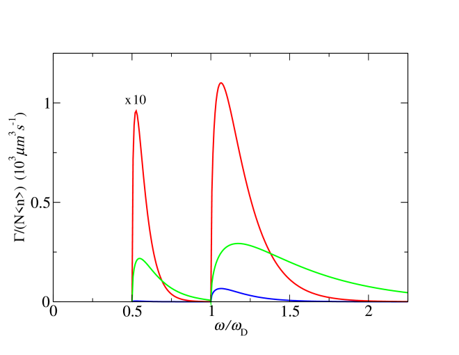
Figure 1: Association rate $\Gamma/N\langle n\rangle$ for a thermal gas of ${}^{7}{\rm Li}$ atoms as a function of the modulation frequency of the magnetic field. The angular frequency $\omega$ is normalized to the angular binding frequency $\omega_{D}$ of the dimer. The bias field is $\bar{B}=734.5$ G, which corresponds to $\bar{a}\approx 1100~{}a_{0}$. The three sets of curves are for different values of the modulation amplitude $b$ and the temperature $T$: $(b,T)$=$(0.57\,{\rm G},3\,{\rm\mu K})$ (highest peak value, red), $(0.57\,{\rm G},10\,{\rm\mu K})$ (green), and $(0.14\,{\rm G},3\,{\rm\mu K})$ (lowest peak value, blue). The association rates in the region $\omega<\omega_{D}$ have been multiplied by 10 to make the subharmonic transitions more visible.

Since the number of atoms in the thermal clouds and the modulation times for each set of $(b,T)$ were not specified in Ref. Hulet1302 , we are unable to make quantitative comparisons with our theoretical results. In Fig. 1, we show our results for the association rates as functions of the angular frequency $\omega$ for the three sets of values of $(b,T)$ for which the atom loss was measured in Ref. Hulet1302 . The ratio of $k_{B}T/\hbar$ to the binding frequency $\omega_{D}=\hbar/m\bar{a}^{2}$ of the dimer is $0.15$ and $0.49$ at the temperatures $3\,{\rm\mu K}$ and $10\,{\rm\mu K}$, respectively. Thus the condition $k_{B}T\ll\hbar^{2}/m\bar{a}^{2}$ is much better satisfied at $3\,{\rm\mu K}$. In Fig. 1, the curves for $\omega>\omega_{D}$ are the harmonic association rates $\Gamma_{1}^{(1)}(\omega)$ in Eq. (30) with $\int d^{3}r\,n_{1}n_{2}$ replaced by $\int d^{3}r\,n^{2}/2$. The curves for $\omega<\omega_{D}$ are the subharmonic association rates $\Gamma_{2}^{(1,1)}(\omega)$ in Eq. (52) with $\int d^{3}r\,n_{1}n_{2}$ replaced by $\int d^{3}r\,n^{2}/2$. The subharmonic association rates $\Gamma_{2}^{(2)}(\omega)$ are completely negligible: their peak values are smaller than those for $\Gamma_{2}^{(1,1)}$ by factors of about $3\times 10^{-5}$. The association rates in Fig. 1 are divided by $\int d^{3}r\,n^{2}(\bm{r})=N\langle n\rangle$ to obtain rates $\Gamma/N\langle n\rangle$ that do not depend on the number of atoms. The angular frequency is normalized to the angular binding frequency $\omega_{D}=\hbar/m\bar{a}^{2}$ of the dimer. The heights of the harmonic and subharmonic peaks for $(b,T)$=$(0.57\,{\rm G},3\,{\rm\mu K})$ are larger than those for $(0.14\,{\rm G},3\,{\rm\mu K})$ by the ratio of the values of $b^{2}$, which is 12.8. The maxima of the harmonic association rates are at angular frequencies $\omega$ that are above the threshold $\omega_{\rm D}$ by approximately $k_{B}T/2\hbar$. The maxima of the subharmonic association rates are at angular frequencies that are above the threshold $\frac{1}{2}\omega_{\rm D}$ by approximately $k_{B}T/4\hbar$. The ratios of the maximum of the harmonic peak to the maximum of the subharmonic peak are 11.4, 190, and 13.8 for $(b,T)$=$(0.57\,{\rm G},3\,{\rm\mu K})$, $(0.14\,{\rm G},3\,{\rm\mu K})$, and $(0.57\,{\rm G},10\,{\rm\mu K})$, respectively. They can be compared to the ratios 11.9, 198, and 24.1 predicted using Eq. (53).

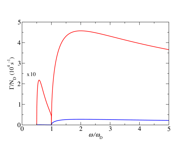
Figure 2: Dissociation rate $\Gamma/N_{D}$ for a thermal gas of ${}^{7}{\rm Li}$ dimers as a function of the angular frequency $\omega$ of the modulated magnetic field. The angular frequency $\omega$ is normalized to the binding angular frequency $\omega_{D}$ of the dimer. The bias field is $\bar{B}=734.5$ G, which corresponds to $\bar{a}\approx 1100~{}a_{0}$. The dissociation rate is independent of the temperature. The two sets of curves are for different values of the modulation amplitude $b$: 0.57 G (higher peak value, red) and 0.14 G (lower peak value, blue). The dissociation rates in the region $\omega<\omega_{D}$ have been multiplied by 10 to make the subharmonic transitions more visible.

Our results for dissociation rates in a thermal gas of dimers as functions of the angular frequency $\omega$ are illustrated in Fig. 1 using the two values of $b$ for which the atom loss was measured in Ref. Hulet1302 . The dissociation rates in Fig. 1 are divided by the number $N_{D}$ of dimers to obtain rates $\Gamma/N_{D}$ that do not depend on $N_{D}$. The angular frequency $\omega$ is normalized to the binding angular frequency $\omega_{D}$ of the dimer. The curves for $\omega>\omega_{D}$ are the harmonic dissociation rates $\Gamma_{1}^{(1)}(\omega)$ in Eq. (39). The curves for $\omega<\omega_{D}$ are the subharmonic dissociation rates $\Gamma_{2}^{(1,1)}(\omega)$ in Eq. (55). The subharmonic association rates $\Gamma_{2}^{(2)}(\omega)$ are completely negligible: their peak values are smaller than those for $\Gamma_{2}^{(1,1)}$ by factors of about $3\times 10^{-5}$. The heights of the harmonic and subharmonic peaks for $b=0.57$ G are larger than those for $b=0.14$ G by the ratio of the values of $b^{2}$, which is 12.8. The maxima of the harmonic association rates are at twice the threshold angular frequency $\hbar/m\bar{a}^{2}$. For large $\omega$, the harmonic rates decrease very slowly as $\omega^{-1/2}$. The maxima of the subharmonic dissociation rates are above the threshold angular frequency $\frac{1}{2}(\hbar/m\bar{a}^{2})$ by only about 0.08 $\hbar/m\bar{a}^{2}$. The ratio of the maximum of the harmonic peak to the maximum of the subharmonic peak is given in Eq. (56). The ratios for $b=0.57$ G and $b=0.14$ G are approximately 21 and 340, respectively.

VIII Comparisons and Summary

In this section, we describe previous theoretical treatments of the association of atoms into dimers using a modulated magnetic field. We then summarize our results on association and dissociation and compare the association results with those from the other approaches.

A theoretical treatment of the association of atoms into dimers using an oscillating magnetic field was presented by Hanna, Köhler, and Burnett in 2007 HKB0609 . They used a two-channel model for the two-atom system, with one channel consisting of atom pairs interacting through a short-range separable potential and a second channel consisting of a single discrete molecular state. The dimer is an eigenstate of the coupled-channel problem. The modulation of the magnetic field was taken into account through the sinusoidal oscillation of the energy of the discrete molecular state. They solved the time-dependent Schrödinger equation for the two-channel model numerically to obtain the probability for association into the dimer as a function of time. They studied the dependence of the association probability for a homogeneous thermal gas on the frequency and amplitude of the oscillating field and on the temperature and density of the gas. Association into dimers in a Bose-Einstein condensate was treated in a completely different way by solving numerically an integro-differential equation for the mean-field of a homogeneous BEC. The results for association probabilities in Ref. HKB0609 are all completely numerical. They can be applied quantitatitively only to homogeneous systems of ⁸⁵Rb and ¹³³Cs atoms under the specific conditions considered in the paper. In order to use their methods to predict the association probability for any other conditions, such as different atoms, other oscillation parameters, different temperature or density for the homogeneous gas, or a trapped gas with variable density, it would be necessary to solve their equations numerically for each set of conditions. Subharmonic transitions were not considered in Ref. HKB0609 .

Brouard and Plata have recently presented a different theoretical treatment of the association of atoms into dimers using an oscillating magnetic field BP1503 . They also used a two-channel model for the two-atom system, with one channel consisting of a continuum of positive-energy atom pair states and the second channel consisting of a single discrete molecular state. The dimer is an eigenstate of the coupled-channel problem. As in Ref. HKB0609 , the modulation of the magnetic field was taken into account through the sinusoidal oscillation of the energy of the discrete molecular state. However in Ref. BP1503 , a time-dependent unitary transformation was used to move the time-dependence into off-diagonal terms between the dimer state and the atom-pair states. They showed that for frequencies near the harmonic resonance, the dynamics in the transformed frame can be approximated by a time-independent Hamiltonian whose entries are given analytically as functions of the oscillation parameters and the Feshbach resonance parameters. Subharmonic transitions in an appropriate transformed frame are described by a different time-independent Hamiltonian whose entries are given analytically. Some qualitative aspects of the association process were deduced from these effective Hamiltonians. However the results in Ref. BP1503 for association probabilities in thermal gases of ⁸⁵Rb atoms and in Bose-Einstein condensates of ⁸⁵Rb atoms are completely numerical.

In this paper, we have applied the new approach to this problem that was introduced in Ref. LSB:1406 . It was based on the realization that the leading effect of an oscillating magnetic field near a Feshbach resonance can be treated as a time-dependent perturbation proportional to the contact operator $C$. In Appendix A, we presented a quantum field theory argument that the perturbation proportional to $C$ can also be used beyond first order. Fermi’s Golden Rule is used to obtain general expressions for transition rates in terms of transition matrix elements of $C$. Our general formula for the harmonic transition rate $\Gamma_{1}^{(1)}(\omega)$ in Eq. (8) comes from the first-order perturbation in $C$ and was obtained previously in Ref. LSB:1406 . There is a contribution $\Gamma_{2}^{(2)}(\omega)$ to the subharmonic transition rate from the first-order perturbation in $C$ that is related in a simple way to the harmonic rate and is given in Eq. (11). However the second-order perturbation in $C$ gives another contribution $\Gamma_{2}^{(1,1)}(\omega)$ to the subharmonic transition rate that is given in Eq. (13). Near the Feshbach resonance, $\Gamma_{2}^{(1,1)}$ is larger than $\Gamma_{2}^{(2)}$ by a factor of $(\bar{a}/a_{\rm bg})^{2}$.

For a homogeneous system, our general expressions for the transition rates can be simplified by expressing the transition matrix elements of the contact operator in terms of transition matrix elements of the contact density operator ${\cal C}$. The harmonic transition rate $\Gamma_{1}^{(1)}$ in Eq. (8) can be simplified by inserting Eq. (16). The subharmonic transition rate $\Gamma_{2}^{(1,1)}$ in Eq. (13) can be simplified by inserting Eq. (17). For a nonhomogeneous system in the local density approximation, these simplifications can first be used to calculate the transition rates for the homogeneous system. Substitutions such as those in Eqs. (18) and (19) can then be used to obtain the transitions rate for the nonhomogenous system.

To obtain association rates in a thermal gas of atoms and dissociation rates in a thermal gas of dimers, we first exploited the low density to reduce the transition matrix elements of ${\cal C}$ in the thermal gas to transition matrix elements of ${\cal C}$ in the two-body problem. Those matrix elements were calculated in Appendix B using the quantum field theory formulation of the problem of atoms with zero-range interactions. In the two-atom sector, this is equivalent to a single-channel model for atoms with large scattering length, with the dimer arising dynamically as a bound state. This allowed us to calculate the matrix elements of the contact density analytically.

Our final results for the harmonic and subharmonic association rates in a thermal gas of atoms are given in Eqs. (30) and (52). Our final results for the harmonic and subharmonic disssociation rates in a thermal gas of dimers are given in Eqs. (39) and (55). These results are analytic functions of all the relevant parameters: the oscillation parameters $\omega$, $b$, and $\bar{a}$ or $\bar{B}$, the Feshbach resonance parameters $a_{\rm bg}$, $B_{0}$, and $\Delta$, and the temperature $T$. The association rates in a thermal gas of fermions with two spin states depend on the local number densities $n_{1}(\bm{r})$ and $n_{2}(\bm{r})$ only through the multiplicative factor $\int d^{3}r\,n_{1}n_{2}$. The dissociation rates in a thermal gas of dimers depend on the local number density $n_{\rm D}(\bm{r})$ only through the multiplicative factor $\int d^{3}r\,n_{\rm D}$. Our analytic results should be useful for analyzing experiments on association into and dissociation of dimers. They should also be useful for designing experiments that optimize the number of dimers created or destroyed by the modulated magnetic field. For a thermal gas of atoms with $k_{B}T\ll\hbar^{2}/m\bar{a}^{2}$, the maximum in the harmonic association rate is at an angular frequency $\omega$ that is above the threshold $\hbar/m\bar{a}^{2}$ by approximately $k_{B}T/2\hbar$. The maximum in the subharmonic association rate is at an angular frequency that is above the threshold $\frac{1}{2}(\hbar/m\bar{a}^{2})$ by approximately $k_{B}T/4\hbar$. For a thermal gas of dimers, the maximum in the harmonic dissociation rate is at an angular frequency $\omega$ that is approximately twice the threshold $\hbar/m\bar{a}^{2}$. The maximum in the subharmonic dissociation rate is at an angular frequency that is above the threshold $\frac{1}{2}(\hbar/m\bar{a}^{2})$ by approximately $0.08\,(\hbar/m\bar{a}^{2})$.

Our general results for the harmonic and subharmonic transition rates in terms of matrix elements of the contact density operator can also be applied to other systems. An analytic result for the association rate in a dilute Bose-Einstein condensate of identical bosons was given in Ref. LSB:1406 . It should also be possible to obtain analytic results for superfluids of fermions with two spin states at zero temperature, including the dissociation rate of dimers in the BEC limit and the dissociation rate of Cooper pairs in the BCS limit. The dissociation rate of paired fermions in the unitary limit is more challenging, but it is an important problem because it would allow the first direct measurements of the gap for the unitary Fermi gas.

Appendix A Quantum Field Theory Derivation of Perturbing Hamiltonian

Particles with a scattering length $a$ that is large compared to the range $r_{0}$ of their interactions can be described by a local quantum field theory. For a fermion with two spin states, there are two fermionic quantum fields $\psi_{1}$ and $\psi_{2}$. The interactions of the quantum field theory are made local by taking the zero-range limit at the expense of introducing an ultraviolet cutoff $\Lambda$ on the momenta of virtual particles. The interaction Hamiltonian density is

$${\cal H}_{\rm int}=(\lambda_{0}/m)\psi_{1}^{\dagger}\psi_{2}^{\dagger}\psi_{2}\psi_{1},$$ (57)

where $\lambda_{0}$ is the bare coupling constant. If $\hbar$ is set to 1, $\lambda_{0}$ has dimensions of length. The field theory describes particles with scattering length $a$ if the bare coupling constant is

$$\lambda_{0}=\frac{4\pi}{1/a-2\Lambda/\pi}.$$ (58)

Matrix elements of the operator $\psi_{1}^{\dagger}\psi_{2}^{\dagger}\psi_{2}\psi_{1}$ diverge as $\Lambda^{2}$ as the cutoff is increased to $\infty$. Since $\lambda_{0}$ scales as $1/\Lambda$, matrix elements of the interaction Hamiltonian density in Eq. (57) therefore diverge as $\Lambda$. In matrix elements of the complete Hamiltonian density, the divergence is cancelled by a corresponding divergence in matrix elements of the kinetic energy density. In matrix elements of the operator $\psi_{1}^{\dagger}\psi_{2}^{\dagger}\psi_{2}\psi_{1}$, subleading terms that diverge as $\Lambda$ give finite contributions to the energy density. The contact density operator in the quantum field theory is Braaten:2008uh

$${\cal C}=\lambda_{0}^{2}\psi_{1}^{\dagger}\psi_{2}^{\dagger}\psi_{2}\psi_{1}.$$ (59)

This operator has finite matrix elements, because the divergence in the matrix element of $\psi_{1}^{\dagger}\psi_{2}^{\dagger}\psi_{2}\psi_{1}$ proportional to $\Lambda^{2}$ is compensated by a factor of $1/\Lambda^{2}$ from $\lambda_{0}^{2}$.

The local quantum field theory can describe particles with a time-dependent scattering length $a(t)$ provided the time scale $a/\dot{a}$ is large compared to the time scale $mr_{0}^{2}/\hbar$ set by the range. In the interaction Hamiltonian density in Eq. (57), the time-dependent bare coupling constant $\lambda_{0}(t)$ is obtained by replacing $a$ in Eq. (58) by $a(t)$. If the time dependence consists of small deviations in the inverse scattering length from some value $1/\bar{a}$, the bare coupling constant can be expanded around the corresponding value $\bar{\lambda}_{0}$:

$$\lambda_{0}(t)=\bar{\lambda}_{0}-\frac{\bar{\lambda}_{0}^{2}}{4\pi}\left(\frac{1}{a(t)}-\frac{1}{\bar{a}}\right)+\frac{\bar{\lambda}_{0}^{3}}{(4\pi)^{2}}\left(\frac{1}{a(t)}-\frac{1}{\bar{a}}\right)^{2}+\ldots.$$ (60)

When this is inserted into the interaction Hamiltonian density in Eq. (57), the term linear in $1/a(t)$ is proportional to the contact density operator in Eq. (59). The term quadratic in $1/a(t)$ is suppressed by $1/\Lambda$ from the additional power of $\bar{\lambda}_{0}$. The higher order terms are even more highly suppressed. Thus the interaction Hamiltonian density in the zero-range limit can be reduced to

$${\cal H}_{\rm int}(t)=\ \frac{\bar{\lambda}_{0}}{m}\psi_{1}^{\dagger}\psi_{2}^{\dagger}\psi_{2}\psi_{1}-\frac{1}{4\pi m}\left(\frac{1}{a(t)}-\frac{1}{\bar{a}}\right){\cal C}.$$ (61)

Appendix B Matrix Elements of the Contact density operator

The field theoretic definition of the contact density operator in Eq. (59) can be expressed as

$${\cal C}(\bm{r})=\phi^{\dagger}(\bm{r})\phi(\bm{r}),$$ (62)

where the contact field $\phi=\lambda_{0}\psi_{2}\psi_{1}$ is a local operator that annihilates two atoms at a point. In the case $a>0$, $\phi(\bm{r})$ has a nonzero amplitude to annihilate a dimer, so it can also be referred to as the dimer field. The transition matrix element of the contact density operator can be expressed as

$$\langle f|{\cal C}({\bm{r}})|i\rangle=\sum_{n}\langle f|\phi^{\dagger}(\bm{r})|n\rangle\langle n|\phi(\bm{r})|i\rangle.$$ (63)

A complete set of states $\sum_{n}|n\rangle\langle n|=1$ has been inserted between $\phi^{\dagger}$ and $\phi$. If only one term in the sum is nonzero, the matrix element factors into a matrix element of $\phi$ that involves the initial state and a matrix element of $\phi^{\dagger}$ that involves the final state.

In order to calculate magneto-transition rates in a thermal gas of atoms or dimers, one needs to calculate transition matrix elements of the contact density operator ${\cal C}(\bm{r})$ between two-atom states, which are either a pair of unbound atoms or a dimer. We will calculate these matrix elements in the Zero-range Model defined by the interaction Hamiltonian density in Eq. (57). The Feynman rules for the atom propagator and the 2-atom–to–2-atom vertex are specified in the appendix of Ref. Braaten:2008uhg . The 2-atom–to–molecule coupling constant $g_{0}$ should be set to 0. Using these Feynman rules, the calculation of transition matrix elements of the contact density operator can be reduced to evaluating Feynman diagrams.

The transition amplitude $A(E_{cm})$ is the amplitude for the transition between a pair of atoms in the asymptotic past and a pair of atoms in the asymptotic future. It is a function only of the energy $E_{\rm cm}$ of the pair of atoms in their center-of-mass frame:

$$E_{\rm cm}=E-K^{2}/4m,$$ (64)

where $E$ is their total energy and $\bm{K}$ is their total momentum. (We set $\hbar=1$ in this Appendix.) The transition amplitude can be calculated by solving the Lippmann-Schwinger equation shown in Figure 3:

$$iA(E_{\rm cm})=-i(\lambda_{0}/m)+(\lambda_{0}/m)I(E_{\rm cm})A(E_{\rm cm}).$$ (65)

The loop integral $I(E_{\rm cm})$ in the last diagram in Figure 3 is

$$I(E_{\rm cm})=\frac{\lambda_{0}^{2}}{m}\int_{\bm{q}}\frac{1}{q^{2}-mE_{\rm cm}-i\epsilon},$$ (66)

where ${\bm{q}}$ is the loop momentum. Using the expression for the bare coupling constant in Eq. (58), the solution can be expressed as

$$A(E_{\rm cm})=\frac{4\pi/m}{-1/a+\sqrt{-mE_{\rm cm}-i\epsilon}}.$$ (67)

This amplitude has a pole in the energy at $E=K^{2}/4m-1/ma^{2}$. The residue of the pole is $-Z_{\rm D}$, where

$$Z_{\rm D}=\ 8\pi/m^{2}a.$$ (68)

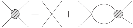
Figure 3: The Lippmann-Schwinger equation for the transition amplitude $A(E_{\rm cm})$. The blob represents $iA(E_{\rm cm})$. The vertex factor is $-i\lambda_{0}/m$.

The standard Feynman rules can be used to calculate matrix elements of local operators between states in the asymptotic past and states in the asymptotic future. However we need matrix elements between initial and final states at the same time. We will use the Feynman rules to calculate matrix elements of the contact field operator $\phi^{\dagger}$ between the vacuum and two-atom states in the asymptotic future. We will then calculate matrix elements of the contact density operator $\phi^{\dagger}\phi$ between two-atom states in the asymptotic future by expressing them in terms of matrix elements of $\phi^{\dagger}$ and $\phi$.

B.1 Vacuum-to-pair matrix element of $\bm{\phi^{\dagger}}$

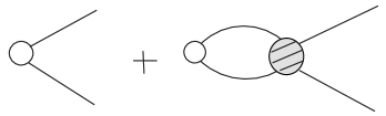
Figure 4: Feynman diagrams for the matrix element of $\phi^{\dagger}(\textbf{r})$ between the vacuum and the atom-pair state $|\bm{K},\bm{k}\rangle$. The open dot represents the $\phi^{\dagger}$ operator, whose Feynman rule is $\lambda_{0}$. The residue of the pole in the energy in the second diagram can be used to determine the matrix element of $\phi^{\dagger}(\textbf{r})$ between the vacuum and the dimer state $|\bm{k_{D}}\rangle$.

The matrix element of $\phi^{\dagger}(\bm{r})$ between the vacuum $|0\rangle$ and an atom-pair state $|\bm{K},\bm{k}\rangle$ with total momentum $\bm{K}$ and relative momentum $\bm{k}$ can be calculated from the Feynman diagrams in Fig. 4. The atoms are on their energy shells with total energy $E=K^{2}/4m+k^{2}/m$. The matrix element is

$$\langle{\bm{K}},{\bm{k}}|\phi^{\dagger}(\textbf{r})|0\rangle = \lambda_{0}\big{[}1+iI(E_{\rm cm})A(E_{\rm cm})\big{]},$$ (69)

$$= -mA(E_{\rm cm}).$$

The energy $E_{\rm cm}$ of the atom pair in their center-of-mass frame depends only on their relative momentum:

$$E_{\rm cm}=k^{2}/m.$$ (70)

B.2 Vacuum-to-dimer matrix element of $\bm{\phi^{\dagger}}$

The matrix element of $\phi^{\dagger}(\bm{r})$ between the vacuum $|0\rangle$ and a dimer state $|{\bm{k}}_{\rm{D}}\rangle$ with momentum ${\bm{k}}_{\rm D}$ can be calculated from second Feynman diagram in Fig. 4. That diagram has a pole in the total energy $E$ of the final-state atoms, which must be off their energy shells. At the pole, the center-of-mass energy is equal to the binding energy of the dimer: $E_{\rm cm}=-1/ma^{2}$. The residue of the pole is the product of the desired matrix element and $Z_{\rm D}^{1/2}$, where $Z_{\rm D}$ is the residue factor given in Eq. (68). The matrix element is therefore

$$\langle{\bm{k}}_{\rm{D}}|\phi^{\dagger}(\textbf{r})|0\rangle = i\lambda_{0}I(E_{\rm cm})(-Z_{\rm D})Z_{\rm D}^{-1/2},$$ (71)

$$= \sqrt{8\pi/a}.$$

B.3 Pair-to-pair matrix element of $\bm{\phi^{\dagger}\phi}$

The matrix element of $\phi^{\dagger}\phi$ between the atom-pair states $|{\bm{K}},{\bm{k}}\rangle$ and $|{\bm{K}^{{}^{\prime}}},{\bm{k}^{{}^{\prime}}}\rangle$ in the asymptotic future can be calculated by inserting a complete set of states between $\phi^{\dagger}$ and $\phi$, as in Eq. (63) . Since the operator $\phi$ annihilates the initial-state atoms, the only term that contributes is the vacuum state. The matrix element factors into the vacuum–to–atom-pair matrix element and its complex conjugate:

$$\langle{\bm{K}^{{}^{\prime}}},{\bm{k}^{{}^{\prime}}}|\phi^{\dagger}(\textbf{r})\phi(\textbf{r})|{\bm{K}},{\bm{k}}\rangle = \langle{\bm{K}^{{}^{\prime}}},{\bm{k}^{{}^{\prime}}}|\phi^{\dagger}(\textbf{r})|0\rangle\langle 0|\phi^{\dagger}(\textbf{r})|{\bm{K}},{\bm{k}}\rangle,$$ (72)

$$= m^{2}A^{*}(E_{\rm cm})A(E^{\prime}_{\rm cm}),$$

where $E_{\rm cm}$ is given in Eq. (64) and $E^{\prime}_{\rm cm}$ is the same expression with $k$ replace by $k^{\prime}$.

The expression for this matrix element given in Ref. Braaten:2008uhg is incorrect: the factor $A^{*}(E_{\rm cm})$ was not complex conjugated. It is easy to see that this is incorrect by setting the final state equal to the initial state: $\bm{K}^{{}^{\prime}}=\bm{K}$, $\bm{k}^{{}^{\prime}}=\bm{k}$. Since the operator is hermitian, the matrix element must be real. This condition is satisfied by Eq. (72). The error made in Ref. Braaten:2008uhg was that the matrix element was calculated not between atom-pair states at the same time, but between an atom-pair state in the asymptotic past and an atom-pair state in the asymptotic future.

B.4 Pair-to-dimer matrix element of $\bm{\phi^{\dagger}\phi}$

The matrix element of $\phi^{\dagger}\phi$ between the atom-pair state $|{\bm{K}},{\bm{k}}\rangle$ in the asymptotic future and the dimer state $|{\bm{k}}_{\rm D}\rangle$ in the asymptotic future can be calculated by inserting a complete set of states between $\phi^{\dagger}$ and $\phi$, as in Eq. (63) . Since the operator $\phi$ annihilates the initial-state atoms, the only term that contributes is the vacuum state. The matrix element factors into a vacuum–to–dimer matrix element and the complex conjugate of a vacuum–to–atom-pair matrix element:

$$\langle{\bm{k}}_{\rm D}|\phi^{\dagger}(\bm{r})\phi(\bm{r})|{\bm{K}},{\bm{k}}\rangle = \langle{\bm{k}}_{\rm D}|\phi^{\dagger}(\textbf{r})|0\rangle\langle 0|\phi(\textbf{r})|{\bm{K}},{\bm{k}}\rangle,$$ (73)

$$= -m\sqrt{8\pi/a}\,A^{*}(E_{\rm cm}),$$

where $E_{\rm cm}$ is given by Eq. (64).

B.5 Dimer-to-dimer matrix element of $\bm{\phi^{\dagger}\phi}$

The matrix element of $\phi^{\dagger}\phi$ between the dimer states $|{\bm{k}}_{\rm D}\rangle$ and $|{\bm{k}}^{\prime}_{\rm D}\rangle$ in the asymptotic future can be calculated by inserting a complete set of states between $\phi^{\dagger}$ and $\phi$, as in Eq. (63). Since the operator $\phi$ annihilates the initial-state dimer, the only term that contributes is the vacuum state. The matrix element factors into a vacuum–to–dimer matrix element and its complex conjugate:

$$\langle{\bm{k}}_{\rm D}^{{}^{\prime}}|\phi^{\dagger}(\bm{r})\phi(\bm{r})|{\bm{k}}_{\rm D}\rangle = \langle{\bm{k}}_{\rm D}^{{}^{\prime}}|\phi^{\dagger}(\bm{r})|0\rangle\langle 0|\phi(\bm{r})|{\bm{k}}_{\rm D}\rangle,$$ (74)

$$= 8\pi/a.$$

References

- (1) S.T. Thompson, E. Hodby, and C.E. Wieman, Phys. Rev. Lett. 95, 190404 (2005) [cond-mat/0505567].
- (2) S.B. Papp and C.E. Wieman, Phys. Rev. Lett. 97, 180404 (2006) [cond-mat/0607667].
- (3) C. Weber, G. Barontini, J. Catani, G. Thalhammer, M. Inguscio, and F. Minardi, Phys. Rev. A 78, 061601(R) (2008) [arXiv:0808.4077].
- (4) A.D. Lange, K. Pilch, A. Prantner, F. Ferlaino, B. Engeser, H.-C. Naegerl, R. Grimm, and C. Chin, Phys. Rev. A 79, 013622 (2009) [arXiv:0810.5503].
- (5) N. Gross, Z. Shotan, O. Machtey, S. Kokkelmans, and L. Khaykovich, Comptes Rendus Physique 12, 4 (2011) [arXiv:1009.0926].
- (6) S.E. Pollack, D. Dries, R.G. Hulet, K.M.F. Magalhaes, E.A.L. Henn, E.R.F. Ramos, M.A. Caracanhas, and V.S. Bagnato, Phys. Rev. A 82, 020701(R) (2010) [arXiv:1004.2887].
- (7) O. Machtey, Z. Shotan, N. Gross, and L. Khaykovich Phys. Rev. Lett. 108, 210406 (2012) [arXiv:1201.2396].
- (8) P. Dyke, S.E. Pollack, and R.G. Hulet, Phys. Rev. A 88, 023625 (2013) [arXiv:1302.0281].
- (9) D.H. Smith, arXiv:1503.02688.
- (10) T.M. Hanna, T. Koehler, and K. Burnett, Phys. Rev. A 75, 013606 (2007) [arXiv:cond-mat/0609725].
- (11) S. Brouard and J. Plata, J. Phys. B: At. Mol. Opt. Phys. 48, 065002 (2015) [arXiv:1503.01700].
- (12) C. Langmack, D.H. Smith, and E. Braaten, Phys. Rev. Lett. 114, 103002 (2015) [arXiv:1406.7313].
- (13) S. Tan, Ann. Phys. 323, 2971 (2008) [cond-mat/0508320].
- (14) E. Braaten and H. -W. Hammer, J. Phys. B 46, 215203 (2013) [arXiv:1302.5617].
- (15) E. Braaten and L. Platter, Phys. Rev. Lett. 100, 205301 (2008) [arXiv:0803.1125].
- (16) E. Braaten, D. Kang, L. Platter, Phys. Rev. A. 78, 053606 (2008) [arXiv:0806.2277].