Searching for a Compressed Polyline
with a Minimum Number of Vertices

Abstract

There are many practical applications that require simplification of polylines. Some of the goals are to reduce the amount of information necessary to store, improve processing time, or simplify editing. The simplification is usually done by removing some of the vertices, making the resultant polyline go through a subset of the source polyline vertices. However, such approaches do not necessarily produce a new polyline with the minimum number of vertices. The approximate solution to find a polyline, within a specified tolerance, with the minimum number of vertices is described in this paper.

I Introduction

The task is to find a polyline, within a specified tolerance of the source polyline, with the minimum number of vertices. That polyline is called optimal. Usually, a subset of vertices of the source polyline is used to construct an optimal polyline [1, 2]. However, an optimal polyline does not necessarily have vertices coincident with the source polyline vertices. One approach, to allow the resultant polyline to have flexibility in the locations of vertices, is to find the intersection between adjacent straight lines [3] or geometrical primitives [4]. However, there are situations when such an approach does not work well, for example, when adjacent straight lines are almost parallel to each other or a circular arc is close to being tangent to a straight segment. The approach described in this paper evaluates a set of vertex locations (considered locations) while searching for a polyline with the minimum number of vertices.

II Algorithm

II-A Discretization of the Solution

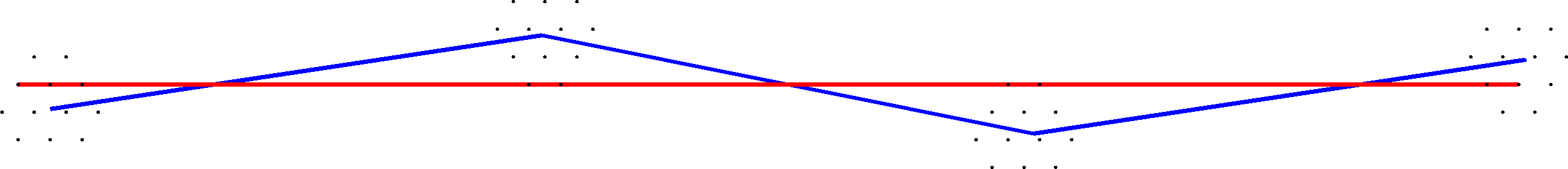
Figure 1: Example of one segment (red segment) between considered locations (black dots) within tolerance of the source polyline (blue polyline).

Any compressed polyline must be within tolerance of the source polyline; therefore, the compressed polyline must have vertices within tolerance of the source polyline. It would be very difficult to consider all possible polylines and find one with the minimum number of vertices; therefore, as an approximation, only some locations around vertices of the source polyline are considered (see the black points around the vertices of the source polyline in Fig. 1).

The locations around vertices of the source polyline are chosen to be on an infinite equilateral triangular grid with the distance from vertices of the source polyline less than the specified tolerance. The equilateral triangular grid (see Fig. 2) has the lowest number of nodes versus other grids (square, hexagonal, etc.), satisfying that distance from any point to the closest node does not exceed the specified threshold.

Figure 2: The worst case distance for the equilateral triangular grid is the distance from the center of the triangle $\displaystyle O$ to any vertex of the equilateral triangle. If $\displaystyle OA=OB=OC=1$, then $\displaystyle AB=BC=CA=\sqrt{3}$.

The choice for the side of an equilateral triangle in the equilateral triangular grid is calculated from the error it introduces. That error can be expressed as a proportion of the specified tolerance. For example, $\displaystyle q\in\left(0,1\right)$ proportion of the specified tolerance means that the side of the equilateral triangle is equal to $\displaystyle q\sqrt{3}$ times the specified tolerance. This leads to about $\displaystyle\dfrac{2\pi}{3\sqrt{3}q^{2}}\approx\dfrac{1.2}{q^{2}}$ locations per each vertex. To decrease complexity, some locations might be skipped; if they are considered in neighbor vertices of the source polyline, however, it should be done without breaking the combinatorial algorithm described in section II-E. If tolerance is great, it is possible to consider locations around segments of the source polyline. In this paper, to support any tolerance, only locations around vertices of the source polyline are considered. Densification of the source polyline might be necessary to find the polyline with the minimum number of vertices.

II-B Testing a Segment to Satisfy Tolerance

For a compressed polyline to be within tolerance, every segment of the compressed polyline must be within tolerance from the part of the source polyline it describes. To find the compressed polyline with the minimum number of vertices, this test has to be performed many times for all combinations of possible locations of vertices (see Fig. 1). [5] describes an efficient approach to perform these tests based on the convex hull. If the convex hull is stored as a polygon, the complexity of this task is $\displaystyle O{\left(\log{n}\right)}$, where $\displaystyle n$ is the number of vertices in the convex hull [5]. The expected complexity of the convex hull for the $\displaystyle N$ random points in any rectangle is $\displaystyle O{\left(\log{N}\right)}$, see [6]. If the source polyline has parts close to an arc, the size of the convex hull tends to increase. For the worst case, the number of vertices in the convex hull is equal to the number of vertices in the original set.

If there are no lines with thickness of two tolerances covering the convex hull completely, then one segment cannot describe this part of the source polyline. The complexity of this check is $\displaystyle O{\left(n\log{n}\right)}$.

A convex hull for any part of the source polyline is constructed in the same way as in [5].

II-C Testing Segment End Points

The test described in the previous section II-B does not check the ends of the segment. The example in Fig. 3 shows that the source polyline changes direction to the opposite several times (zigzag) before going up. Without checking end points and changes in direction, the compressed polyline might not describe some parts of the source polyline (Fig. 3a). Therefore, these tests are necessary to guarantee that the compressed polyline (Fig. 3b) describes the source polyline without missing any parts.

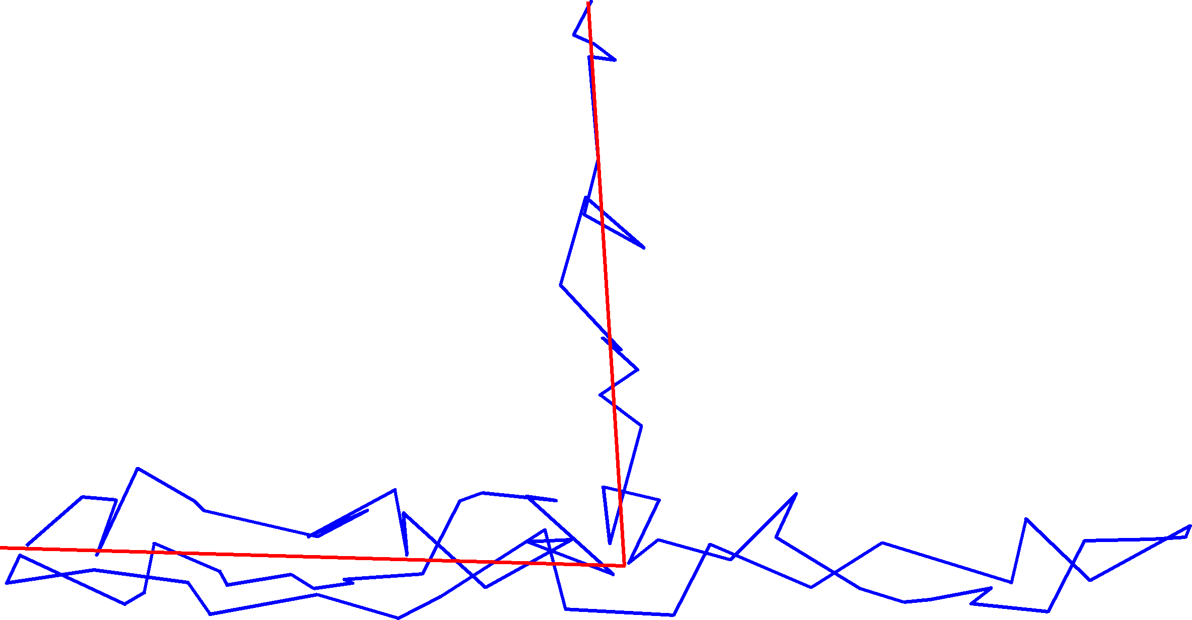
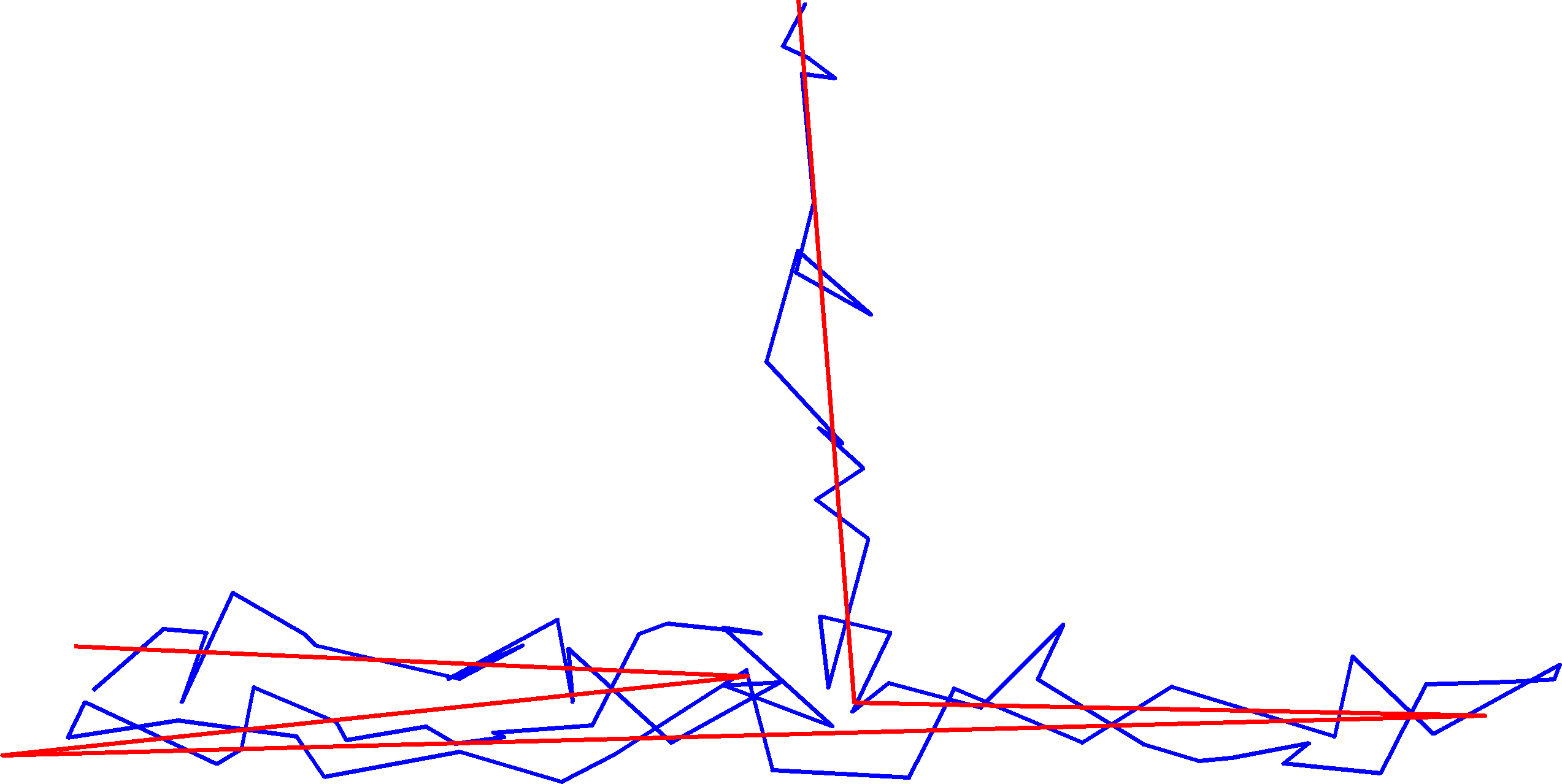
(a)	(b)

Figure 3: The blue polyline is the source polyline. The red polyline is the result of the algorithm without checking for end points and the source polyline direction (a) and with both checks performed (b).

The segment end points to be within the tolerance of the part of the source polyline are tested based on the convex hull in the same way as the test for the segment to be within tolerance performed in section II-B.

This is equivalent to the test if the segment extended in parallel and perpendicular directions by the tolerance (see Fig. 4) contains a convex hull of the part of the source polyline it describes. If more directions are used, a better approximation of the curved polygon can be obtained. The complexity of the test is $\displaystyle O{\left(\log{n}\right)}$.

Figure 4: The diagonal striped area is the tolerance area around the segment. The thin rectangle is the approximation of the area around the segment. A thick polygon would be a better approximation.

II-D Testing Polyline Direction

The test for the source polyline to have a zigzag is performed by checking if the projection to the segment of backward movement exceeds two tolerances ($\displaystyle 2T$, where $\displaystyle T$ is the tolerance). Two tolerances are used because one vertex of the source polyline can shift forward by the tolerance and the vertex after that shift backward by the tolerance. The algorithm is based on analyzing zigzags before the processed point. Let $\displaystyle p_{i}$ be the vertices of the polyline, $\displaystyle i=\overline{0..N-1}$, $\displaystyle N$ be the number of vertices in the polyline. The next algorithm constructs a table for efficient testing.

1. Define a set of directions $\displaystyle\alpha_{j}=\dfrac{2\pi}{N_{d}}j$,
   where $\displaystyle j=\overline{0..N_{d}-1}$, $\displaystyle N_{d}$ is the number of directions.

2. Cycle over each direction $\displaystyle\alpha_{j}$, $\displaystyle j=\overline{0..N_{d}-1}$.

   1. Define the priority queue with requests containing two numbers. The first number is the real value, and the second number is the index. Priority of the request is equal to the first number.

   2. Set $\displaystyle k=0$.

   3. Cycle over each point $\displaystyle p_{i}$ of the source polyline,
      $\displaystyle i=\overline{0..N-1}$.

      1. Calculate projection of $\displaystyle p_{i}$ to the direction $\displaystyle\alpha_{j}$ (scalar product between the point and the direction vector):

         $$d=p_{i}\cdot\left(\cos\left(\alpha_{j}\right),\sin\left(\alpha_{j}\right)\right).$$

      2. Remove all requests from the priority queue with a priority of more than $\displaystyle d+2T$. If the largest index from removed requests is larger than $\displaystyle k$, set $\displaystyle k$ equal to that index.

      3. Set $\displaystyle V_{j,i}=k$.

      4. Add request $\displaystyle\left(d,i+1\right)$ to the priority queue.

To test if the part of the source polyline between vertices $\displaystyle i_{s}$ and $\displaystyle i_{e}$ has a zigzag.

1. First, find the closest direction $\displaystyle\alpha_{j}$ to the direction of the segment $\displaystyle\alpha_{j^{*}}$: $\displaystyle j^{*}=\operatorname{round}{\left(\dfrac{N_{d}}{2\pi}\alpha\right)}\!\!\!\mod N_{d}$, where $\displaystyle\alpha$ is the direction of the segment.

2. Second, if $\displaystyle V_{j^{*},i_{e}}\leq i_{s}$, then there are no zigzags for the segment describing the part of the source polyline from vertex $\displaystyle i_{s}$ till $\displaystyle i_{e}$.

Let $\displaystyle W_{i}=\min_{0\leq j\wedge j<N_{d}}{\left(V_{j,i}\right)}$. If $\displaystyle i_{s}<W_{i_{e}}$, then one segment cannot describe the part of the source polyline from vertex $\displaystyle i_{s}$ till $\displaystyle i_{e}$.

This test has some limitations:

• The tested direction is approximated by the closest one, making the check approximate.

• For some error models, a zigzag might pass the test. For example, if errors are limited by a circle, a zigzag by two tolerances is only possible if it happens directly on the segment.

Nevertheless, it is an efficient test to avoid absurd results, like in Fig. 3a. The complexity of the algorithm is $\displaystyle O{\left(N_{d}N\log\left(N\right)\right)}$ and the complexity to test any segment is $\displaystyle O{\left(1\right)}$.

II-E Combinatorial Approach to Find an Optimal Solution

The optimal solution is found by using the algorithm described in [3].

Let $\displaystyle p_{i,j}$ be considered locations for vertex $\displaystyle p_{i}$, where $\displaystyle{i=\overline{0..N-1}}$, $\displaystyle{j=\overline{0..N_{i}-1}}$, $\displaystyle N_{i}$ is the number of considered locations for the vertex $\displaystyle i$. Let pairs $\displaystyle\left(i_{k},j_{k}\right)$, $\displaystyle{k=\overline{0..m}}$, divide the source polyline into $\displaystyle m$ straight segments $\displaystyle\left(p_{i_{k},j_{k}},p_{i_{k+1},j_{k+1}}\right)$ describing the source polyline from vertex $\displaystyle i_{k}$ till $\displaystyle i_{k+1}$, $\displaystyle k=\overline{0..m-1}$. Notice that neighbor segments are already connected in $\displaystyle p_{i_{k},j_{k}}$, $\displaystyle k=\overline{1..m-1}$, and this solution avoids problems in algorithms [3, 4] when the intersection of neighbor segments is far away from the source polyline.

The goal of this algorithm is to find the solution with the minimum number of vertices while satisfying tolerance restriction, and among them with the minimum integral square differences. Therefore, minimization is performed in two parts $\displaystyle\left\{\begin{aligned} &T^{\#}\\ &T^{\epsilon}\end{aligned}\right\}$, where the first part $\displaystyle T^{\#}$ is the number of segments, and the second part $\displaystyle T^{\epsilon}$ is the integral of the square deviation between segments and the source polyline. The solutions are compared by the number of segments and, if they have the same number of segments, by square deviation between segments and the source polyline. The solution of this task, when the optimal polyline has vertices coincident with the source polyline, can be found in [7].

Let $\displaystyle P_{k}$, $\displaystyle k=\overline{0..N-1}$ be parts of the source polyline from vertex $\displaystyle 0$ to $\displaystyle k$.

The optimal solution is found by induction. Define the optimal solution for polyline $\displaystyle P_{0}$ as $\displaystyle\left\{\begin{aligned} &T_{0,j}^{\#}\\ &T_{0,j}^{\epsilon}\end{aligned}\right\}=\left\{\begin{aligned} 0\\ 0\end{aligned}\right\}$, $\displaystyle{j=\overline{0,N_{0}-1}}$. For $\displaystyle k=\overline{1,N-1}$, construct the optimal solution for $\displaystyle P_{k}$ from optimal solutions for $\displaystyle P_{k^{\prime}}$, $\displaystyle k^{\prime}=\overline{0..k-1}$.

$$\left\{\begin{aligned} &T_{k,j}^{\#}\\ &T_{k,j}^{\epsilon}\end{aligned}\right\}=\min_{\begin{aligned} 0\leq k^{\prime}\wedge k^{\prime}<k\\ 0\leq j^{\prime}\wedge j^{\prime}<N_{k^{\prime}}\\ \operatorname{check}{\left(\left(k^{\prime},j^{\prime}\right),\left(k,j\right)\right)}\end{aligned}}{\left(\left\{\begin{aligned} &T_{k^{\prime},j^{\prime}}^{\#}+1\\ &T_{k^{\prime},j^{\prime}}^{\epsilon}+\epsilon_{\left(k^{\prime},j^{\prime}\right),\left(k,j\right)}\end{aligned}\right\}\right)},$$

where $\displaystyle\epsilon_{\left(k^{\prime},j^{\prime}\right),\left(k,j\right)}$ is the integral square difference between segment $\displaystyle\left(p_{k^{\prime},j^{\prime}},p_{k,j}\right)$ and the source polyline from vertex $\displaystyle k^{\prime}$ till $\displaystyle k$, $\displaystyle\operatorname{check}{\left(\left(k^{\prime},j^{\prime}\right),\left(k,j\right)\right)}$ is a combination of checks described in the previous sections II-B, II-C, and II-D to check if segment $\displaystyle\left(p_{k^{\prime},j^{\prime}},p_{k,j}\right)$ can describe the part of the source polyline from vertex $\displaystyle k^{\prime}$ till $\displaystyle k$.

To reconstruct the optimal solution, it is necessary for $\displaystyle\left\{\begin{aligned} &T_{k,j}^{\#}\\ &T_{k,j}^{\epsilon}\end{aligned}\right\}$ to store $\displaystyle\left\{k^{\prime},j^{\prime}\right\}$ when the right part is minimal.

The optimal solution is reconstructed from

$$\min_{0\leq j\wedge j<N_{N-1}}{\left\{\begin{aligned} &T_{N-1,j}^{\#}\\ &T_{N-1,j}^{\epsilon}\end{aligned}\right\}}$$

by recurrently using stored $\displaystyle\left\{k^{\prime},j^{\prime}\right\}$ values.

II-F Optimization

It is possible to significantly reduce the complexity of the algorithm described in the previous section II-E by using the approach described in [3].

$$\min_{\begin{aligned} k_{1}\leq k^{\prime}\wedge k^{\prime}\leq k_{2}\\ 0\leq j^{\prime}\wedge j^{\prime}<N_{k^{\prime}}\\ \operatorname{check}{\left(\left(k^{\prime},j^{\prime}\right),\left(k,j\right)\right)}\end{aligned}}{\left(\left\{\begin{aligned} &T_{k^{\prime},j^{\prime}}^{\#}+1\\ &T_{k^{\prime},j^{\prime}}^{\epsilon}+\epsilon_{\left(k^{\prime},j^{\prime}\right),\left(k,j\right)}\end{aligned}\right\}\right)}\gtrapprox$$ (1)

$$\gtrapprox \min_{\begin{aligned} k_{1}\leq k^{\prime}\wedge k^{\prime}\leq k_{2}\\ 0\leq j^{\prime}\wedge j^{\prime}<N_{k^{\prime}}\end{aligned}}{\left(\left\{\begin{aligned} &T_{k^{\prime},j^{\prime}}^{\#}+1\\ &T_{k^{\prime},j^{\prime}}^{\epsilon}+\epsilon_{\left(k^{\prime},j^{\prime}\right),\left(k,j\right)}^{\left(k_{2}\right)}\end{aligned}\right\}\right)},$$

where

$$\epsilon_{\left(k^{\prime},j^{\prime}\right),\left(k,j\right)}^{\left(k_{2}\right)}=\\ =\min_{\begin{aligned} 0\leq j_{2}\wedge j_{2}<N_{k_{2}}\\ \operatorname{check}{\left(\left(k^{\prime},j^{\prime}\right),\left(k_{2},j_{2}\right)\right)}\\ \operatorname{check}{\left(\left(k_{2},j_{2}\right),\left(k,j\right)\right)}\end{aligned}}{\left(\epsilon_{\left(k^{\prime},j^{\prime}\right),\left(k_{2},j_{2}\right)}+\epsilon_{\left(k_{2},j_{2}\right),\left(k,j\right)}\right)}.$$

From (1), it follows that

$$\min_{\begin{aligned} k_{1}\leq k^{\prime}\wedge k^{\prime}\leq k_{2}\\ 0\leq j^{\prime}\wedge j^{\prime}<N_{k^{\prime}}\\ \operatorname{check}{\left(\left(k^{\prime},j^{\prime}\right),\left(k,j\right)\right)}\end{aligned}}{\left(\left\{\begin{aligned} &T_{k^{\prime},j^{\prime}}^{\#}+1\\ &T_{k^{\prime},j^{\prime}}^{\epsilon}+\epsilon_{\left(k^{\prime},j^{\prime}\right),\left(k,j\right)}\end{aligned}\right\}\right)}\gtrapprox$$ (2)

$$\gtrapprox \min_{\begin{aligned} 0\leq j_{2}\wedge j_{2}<N_{k_{2}}\\ \operatorname{check}{\left(\left(k_{2},j_{2}\right),\left(k,j\right)\right)}\end{aligned}}{\left(\left\{\begin{aligned} &T_{k_{2},j_{2}}^{\#}\\ &T_{k_{2},j_{2}}^{\epsilon}+\epsilon_{\left(k_{2},j_{2}\right),\left(k,j\right)}\end{aligned}\right\}\right)}$$

and

$$\min_{\begin{aligned} k_{1}\leq k^{\prime}\wedge k^{\prime}\leq k_{2}\\ 0\leq j^{\prime}\wedge j^{\prime}<N_{k^{\prime}}\\ \operatorname{check}{\left(\left(k^{\prime},j^{\prime}\right),\left(k,j\right)\right)}\end{aligned}}{\left(\left\{\begin{aligned} &T_{k^{\prime},j^{\prime}}^{\#}+1\\ &T_{k^{\prime},j^{\prime}}^{\epsilon}+\epsilon_{\left(k^{\prime},j^{\prime}\right),\left(k,j\right)}\end{aligned}\right\}\right)}\gtrapprox$$ (3)

$$\gtrapprox \min_{0\leq j_{1}\wedge j_{1}<N_{k_{1}}}{\left(\left\{\begin{aligned} &T_{k_{1},j_{1}}^{\#}\\ &T_{k_{1},j_{1}}^{\epsilon}\end{aligned}\right\}\right)}+$$

$$+\left\{\begin{aligned} &\>\>\>\>\>\>\>\>\>\>\>\>\>\>\>\>\>\>\>\>\>\>\>\>\>\>\>\>\>1\\ &\min_{\begin{aligned} 0\leq j_{2}\wedge j_{2}<N_{k_{2}}\\ \operatorname{check}{\left(\left(k_{2},j_{2}\right),\left(k,j\right)\right)}\end{aligned}}{\left(\epsilon_{\left(k_{2},j_{2}\right),\left(k,j\right)}\right)}\end{aligned}\right\}.$$

The maximum of (2) and (3) can be used to skip checking combinations between vertex $\displaystyle k_{1}$ and $\displaystyle k_{2}$.

The inequalities (2) and (3) are approximate due to the use of considered locations. However, this allows finding stricter limitations for the solution inside the interval and simultaneously finding the solution for breaking at vertex $\displaystyle k_{2}$.

It is possible to construct (2) and (3) with exact inequalities by constructing the optimal solution when the end point is not required to end in the considered location. Similarly, the part from vertex $\displaystyle k_{2}$ to $\displaystyle\left(k,j\right)$ should not be required to end in considered locations for vertex $\displaystyle k_{2}$. This is useful when the resultant polyline is required to go through the vertices of the source polyline. However, such an algorithm has a worse compression ratio than the one with the flexibility in joints.

See paper [3] for further details of this algorithm.

II-G Optimal Compression of Closed Polylines

To find the optimal compression of a closed polyline, it is necessary to know the starting vertex. It is also necessary that the resultant polyline starts and ends in the same vertex. The next algorithm will be used to find the starting vertex and construct a closed resultant polyline.

1. Construct a convex hull for all vertices of the source polyline.

2. Find the smallest angle of the convex hull polygon.

3. Take the vertex corresponding to the smallest angle as the starting vertex and reorient the closed polyline to start from that vertex.

4. Apply the algorithm.

5. From the constructed solution, take one vertex in the middle as the new starting vertex and reorient the closed polyline to start from that vertex.

6. Apply the algorithm once more, while for the first and the last vertex consider only the location of the previous solution for the middle vertex.

Steps 1, 2, and 3 are important for a small closed polyline. For the small closed polyline, the resultant polyline is within tolerance of the source polyline, even with suboptimal orientation. As a consequence, without these steps, step 5 may not find the optimal division of the source polyline, leading to a suboptimal solution.

II-H Optimal Compression by Straight Segments and Arcs

This algorithm is extendible to support arcs. The arc passing through considered locations differs from the segment by the necessity to define the radius. Unfortunately, it adds significant complexity to the algorithm. Nevertheless, such an algorithm is possible. There are different ways to fit an arc to a polyline: minimum integral square differences of squares [8, 9], minimum integral square differences [10, 11, 12, 13, 14], minimum deviation, etc. Algorithms with complexity $\displaystyle O{\left(n\right)}$, where $\displaystyle n$ is the number of vertices in the fitted polyline, are not suitable due to the significant increase in complexity. The algorithms with acceptable complexity $\displaystyle O{\left(1\right)}$ are [8, 9, 13, 14]; however, algorithms based on integral square differences of squares [8, 9] might break for small arcs and, therefore, are not suitable. Checking that the part of the source polyline is within tolerance, end points, and zigzag will be time-consuming due to complexity $\displaystyle O{\left(n\right)}$.

III Analysis of the Algorithm Complexity

The algorithm contains three steps:

1. Preprocessing: construction of convex hulls (section II-B) and filling arrays for an efficient zigzag test (section II-D).

2. Construction of the optimal solution (section II-E).

3. Reconstruction of the optimal solution (section II-E).

A significant amount of time is spent on constructing an optimal solution. It is difficult to evaluate the complexity described in section II-F; however, the worst complexity is

$$O{\left(N^{2}\cdot\max_{0\leq i\wedge i<N}{\left(N_{i}^{2}\right)}\cdot\log{\left(N\right)}\right)}.$$ (4)

The complexity of the algorithm depends on the type of polyline it processes. It is very difficult to conclude what is the practical complexity of this algorithm. If the optimal polyline does not have segments describing too many vertices of the source polyline, (4) tends to be

$$O{\left(N\cdot\max_{0\leq i\wedge i<N}{\left(N_{i}^{2}\right)}\right)}.$$ (5)

Fig. 5 shows how much time it takes to process a polyline depending on the number of vertices. The dependence is very close to linear, supporting (5).

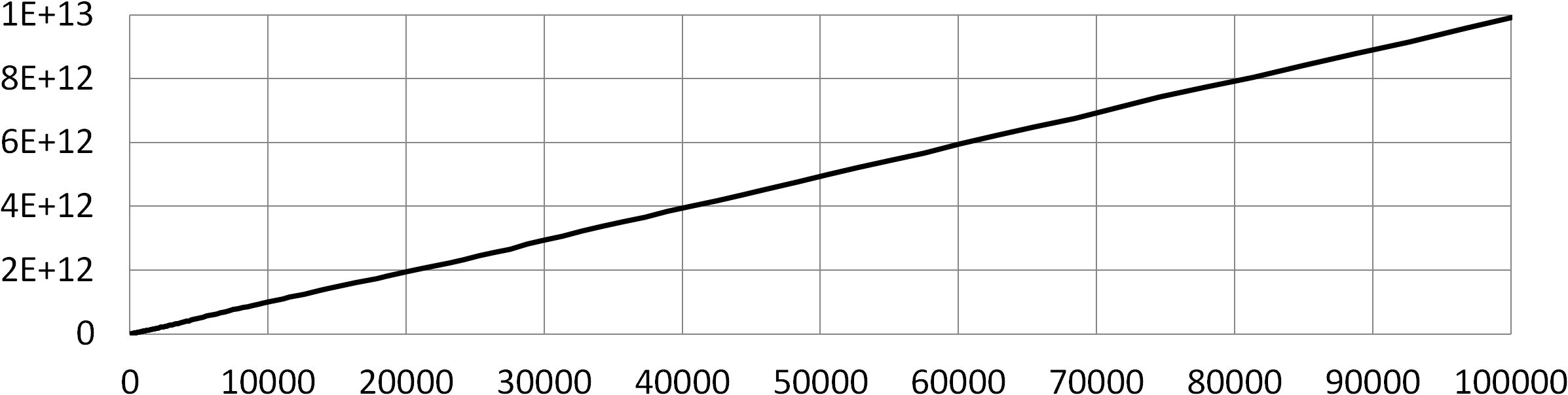
Figure 5: Time needed to process a polyline versus the number of vertices. The time is measured in CPU ticks on the processor Intel Xeon CPU E5-2670. The polylines are generated by the Brownian motion process. Each next vertex is randomly incremented from the previous vertex by random vector, with components normally distributed with zero mean and $\displaystyle 0.25$ standard deviation. The tolerance was set to one. The average reduction in the number of vertices is about $\displaystyle 50$ times.

IV Examples

Fig. 6 shows an example of the algorithm described in this paper. If the source polyline is the noisy version of a ground truth polyline, where the noise does not exceed some threshold, and the algorithm is provided with a tolerance slightly greater than the threshold to account for approximations inside the algorithm, then the resultant polyline will never have more vertices than the ground truth polyline.

(a) (b) (c)

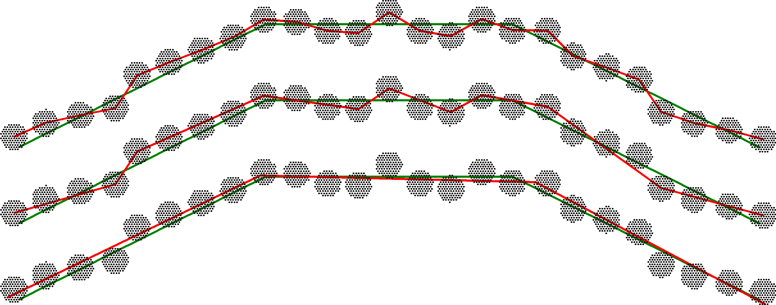
Figure 6: Comparison of the result of approximation of the Douglas-Peucker algorithm (b) and approximation of optimal polyline compression (c). The green polyline is a ground truth. The red polyline is the source polyline (a), the result of the Douglas-Peucker algorithm [1] (b), and the result of optimal polyline compression (c). The black dots around vertices of the source polyline are considered locations for the vertices of the compressed polyline. The vertices of the source polyline are deviated from the segments of the ground truth polyline by random values uniformly distributed in the interval $\displaystyle\left(-0.1,0.1\right)$.

The effectiveness of the approach is shown in Fig. 7. Nine segments are sufficient to represent the arc with specified precision. The algorithm not only optimizes the number of segments, it also finds the locations of the segments that minimize integral square differences. Therefore, as shown in Fig. 7, the algorithm tends to construct segments similar in length.

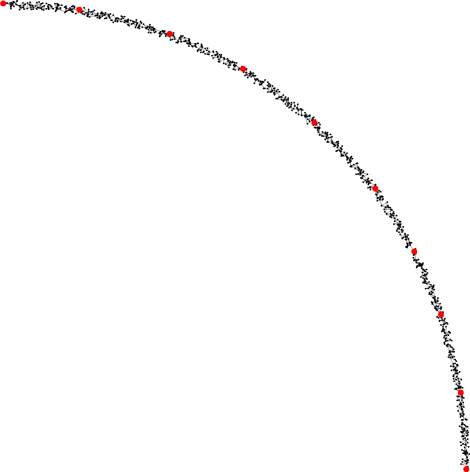
Figure 7: The black polyline is the source polyline. The red circles are the vertices of the optimal polyline. Ground truth is the arc of $\displaystyle 90\degree$. The noise has uniform distribution in the circle of one percent of the arc radius.

Fig. 8 shows the dependence from the error introduced by a discrete set of considered locations (see section II-A) to the efficiency of the compression. Flexibility in places where neighboring segments connect each other is very important to reach maximum compression, especially for noisy data.

V Optimal Compression by Orthogonal Directions

The triangular grid for considered locations supports directions by $\displaystyle 30\degree$. Reconstruction of orthogonal buildings requires support for $\displaystyle 90\degree$ [15] and sometimes $\displaystyle 45\degree$. The square grid for considered locations is more appropriate for this task.

Notice that because only certain directions are allowed, only segments between pairs of considered locations aligned by these directions may be parts of the resultant polyline. Suppose that the resultant segment goes between vertex $\displaystyle i$ and $\displaystyle j$. Because it has to be within tolerance for all vertices between $\displaystyle i$ and $\displaystyle j$, it goes through their considered locations (with the exception of the segment deviating close to the tolerance due to discretization of considered locations).

The optimal solution is found by induction. Define the optimal solution for polyline $\displaystyle P_{0}$ as $\displaystyle\left\{\begin{aligned} &T_{0,j,q}^{\#}\\ &T_{0,j,q}^{\epsilon}\end{aligned}\right\}=\left\{\begin{aligned} 0\\ 0\end{aligned}\right\}$, where $\displaystyle j=\overline{0,N_{0}-1}$, $\displaystyle q=\overline{0,M-1}$, and $\displaystyle M$ is the number of different directions. For orthogonal case $\displaystyle M=4$, and for $\displaystyle 45\degree$ case $\displaystyle M=8$. Take directions as $\displaystyle\alpha_{i}=\dfrac{360\degree}{M}\cdot i$, $\displaystyle i=\overline{0,M-1}$. For $\displaystyle k=\overline{1,N-1}$, construct the optimal solution for $\displaystyle P_{k}$ from the optimal solution for $\displaystyle P_{k-1}$.

$$\left\{\begin{aligned} &T_{k,j,q}^{\#}\\ &T_{k,j,q}^{\epsilon}\end{aligned}\right\}=\\ \min_{\begin{aligned} 0\leq j^{\prime}\wedge j^{\prime}<N_{k-1}\\ 0\leq q^{\prime}\wedge q^{\prime}<M\\ 2\left|q^{\prime}-q\right|\neq M\\ \operatorname{angle}{\left(p_{k,j}-p_{k-1,j^{\prime}},\alpha_{q^{\prime}}\right)}\end{aligned}}{\left(\left\{\begin{aligned} &T_{k-1,j^{\prime},q^{\prime}}^{\#}+\delta_{q^{\prime}\neq q}\\ &T_{k-1,j^{\prime},q^{\prime}}^{\epsilon}+\epsilon_{\left(k-1,j^{\prime}\right),\left(k,j\right)}\end{aligned}\right\}\right)},$$

were $\displaystyle\delta_{q^{\prime}\neq q}=\left\{\begin{aligned} 1,&\text{ if }q^{\prime}\neq q,\\ 0,&\text{ otherwise};\end{aligned}\right.$
$\displaystyle\operatorname{angle}{\left(v,\alpha\right)}$ is the check that the vector $\displaystyle v$ has angle $\displaystyle\alpha$ (zero length vectors are allowed).

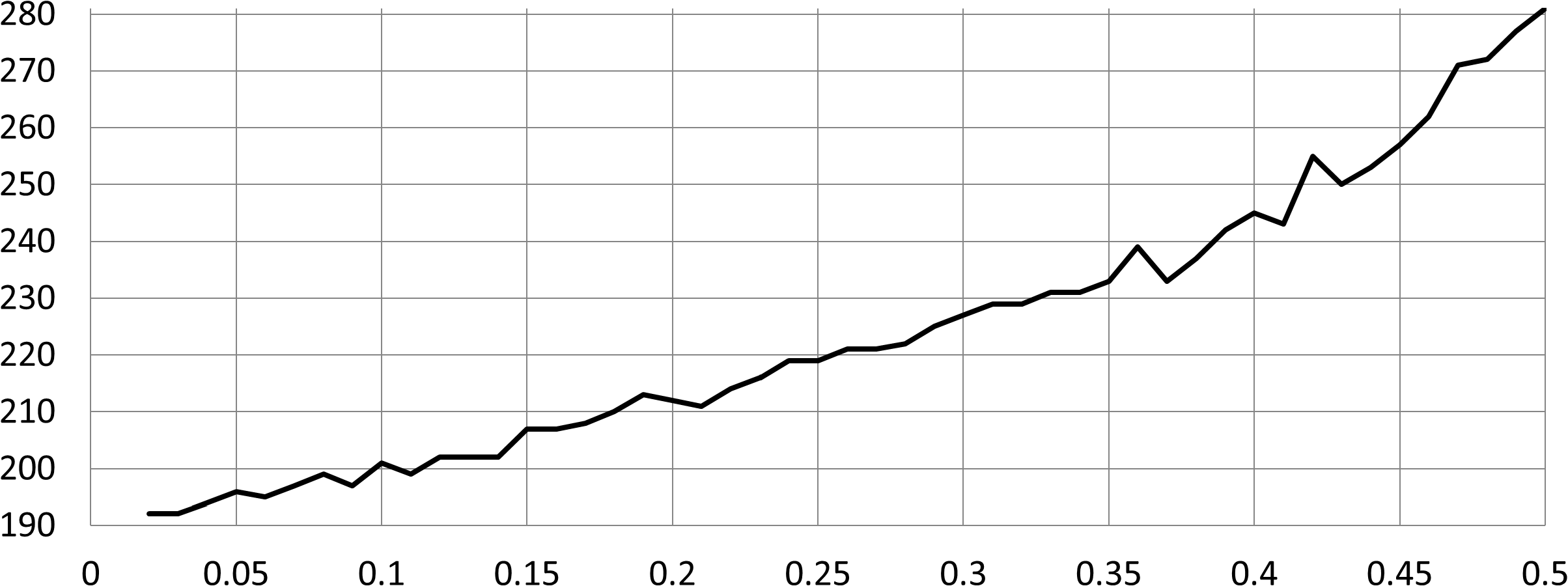
Figure 8: The number of segments versus discretization error. The polyline was generated by the Brownian motion process in the same way as in Fig. 5 with $\displaystyle 10,000$ vertices.

The condition $\displaystyle 2\left|q^{\prime}-q\right|\neq M$ corresponds to prohibiting changes in direction by $\displaystyle 180\degree$.

For the $\displaystyle 45\degree$ case, it is possible to restrict the resultant polyline from having sharp angles by not allowing a change of direction by $\displaystyle 135\degree$ ($\displaystyle\left|4-\left(\left(q^{\prime}-q\right)\bmod 8\right)\right|\neq 1$).

Notice that there are no checks for the tolerance, direction, and end points because they are satisfied during each induction step.

Analyzing the previous solution along $\displaystyle M$ direction will further reduce the amount of calculations. The total complexity of the algorithm is

$$O{\left(N\cdot\max_{0\leq i\wedge i<N}{\left(N_{i}\right)}\cdot M\right)}.$$

For some data, the algorithm may produce an improper result. This happens when the introduction of a zero length segment lowers the penalty.

Because the correct orientation is not known in advance, it is necessary to rotate polylines by different angles and take the solution with the lowest penalty [15, see section 6].

Fig. 9 shows an example for the reconstruction of orthogonal buildings.

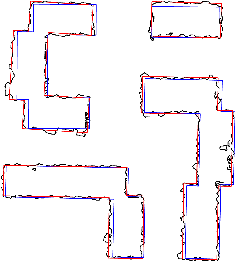
Figure 9: The black polylines are reconstructed buildings from lidar data [16]. The red polylines are the resultant orthogonal shapes. The blue polylines are the ground truth taken from [17].

The reconstruction of buildings with $\displaystyle 45\degree$ sides are shown in Fig. 10.

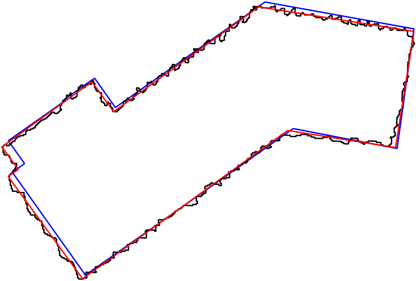
Figure 10: This differs from Fig. 9 by the allowance of $\displaystyle 45\degree$ segments.

The main difference of the algorithm described in this section and [15] is in the parameters. The specification of the tolerance is easier than the specification of the penalty $\displaystyle\Delta$ for each additional segment.

VI Conclusion

This paper describes an approximation algorithm that finds a polyline with the minimum number of vertices while satisfying tolerance restriction. The solution is optimal with the following limitations:

• The vertices of the compressed polyline are limited to considered locations (section II-A).

• The test that the vertex of the compressed polyline is located between some vertices of the source polyline is approximate due to the snapping of the breaking point (section II-F).

• The tests for end points (section II-C) and zigzags are approximate (section II-D).

The performance of the algorithm can be greatly improved if the number of considered locations is decreased without losing quality. This requires further research.

References

- [1] D. H. Douglas and T. K. Peucker, Algorithms for the Reduction of the Number of Points Required to Represent a Digitized Line or its Caricature. The Canadian Cartographer, 1973, vol. 10, no. 2, pp. 112–122.
- [2] F. Chen and H. Ren, “Comparison of vector data compression algorithms in mobile GIS,” in 2010 3rd IEEE International Conference on Computer Science and Information Technology (ICCSIT), vol. 1, July 2010, pp. 613–617. [Online]. Available: http://dx.doi.org/10.1109/ICCSIT.2010.5564118
- [3] A. Gribov and E. Bodansky, “A new method of polyline approximation,” in Structural, Syntactic, and Statistical Pattern Recognition, ser. Lecture Notes in Computer Science, A. Fred, T. M. Caelli, R. P. Duin, A. Campilho, and D. de Ridder, Eds. Springer Berlin Heidelberg, 2004, vol. 3138, pp. 504–511. [Online]. Available: http://dx.doi.org/10.1007/978-3-540-27868-9_54
- [4] E. Bodansky and A. Gribov, “Approximation of a polyline with a sequence of geometric primitives,” in Image Analysis and Recognition, ser. Lecture Notes in Computer Science, A. Campilho and M. Kamel, Eds. Springer Berlin Heidelberg, 2006, vol. 4142, pp. 468–478. [Online]. Available: http://dx.doi.org/10.1007/11867661_42
- [5] J. Hershberger and J. Snoeyink, “Speeding up the Douglas-Peucker line-simplification algorithm,” in Proceedings of the 5th International Symposium on Spatial Data Handling, 1992, pp. 134–143.
- [6] S. Har-Peled, “On the expected complexity of random convex hulls,” CoRR, vol. abs/1111.5340, December 2011. [Online]. Available: http://arxiv.org/abs/1111.5340
- [7] W. S. Chan and F. Chin, “Approximation of polygonal curves with minimum number of line segments or minimum error,” International Journal of Computational Geometry & Applications, vol. 06, no. 01, pp. 59–77, 1996. [Online]. Available: http://dx.doi.org/10.1142/S0218195996000058
- [8] S. M. Thomas and Y. T. Chan, “A simple approach for the estimation of circular arc center and its radius,” Computer Vision, Graphics, and Image Processing, vol. 45, no. 3, pp. 362–370, March 1989. [Online]. Available: http://dx.doi.org/10.1016/0734-189X(89)90088-1
- [9] C. Ichoku, B. Deffontaines, and J. Chorowicz, “Segmentation of digital plane curves: A dynamic focusing approach,” Pattern Recogn. Lett., vol. 17, no. 7, pp. 741–750, June 1996. [Online]. Available: http://dx.doi.org/10.1016/0167-8655(96)00015-3
- [10] S. M. Robinson, “Fitting spheres by the method of least squares,” Commun. ACM, vol. 4, no. 11, p. 491, November 1961. [Online]. Available: http://doi.acm.org/10.1145/366813.366824
- [11] U. M. Landau, “Estimation of a circular arc center and its radius,” Computer Vision, Graphics, and Image Processing, vol. 38, no. 3, pp. 317–326, June 1987. [Online]. Available: http://dx.doi.org/10.1016/0734-189X(87)90116-2
- [12] E. Bodansky and A. Gribov, “Approximation of polylines with circular arcs,” in Graphics Recognition. Recent Advances and Perspectives, ser. Lecture Notes in Computer Science, J. Lladós and Y.-B. Kwon, Eds. Springer Berlin Heidelberg, 2004, vol. 3088, pp. 193–198. [Online]. Available: http://dx.doi.org/10.1007/978-3-540-25977-0_18
- [13] L. Dorst, “Total least squares fitting of k-spheres in n-d Euclidean space using an (n+2)-d isometric representation,” Journal of Mathematical Imaging and Vision, vol. 50, no. 3, pp. 214–234, 2014. [Online]. Available: http://doi.org/10.1007/s10851-014-0495-2
- [14] A. Gribov, “Approximate fitting of circular arcs when two points are known,” 2015, in preparation for http://arxiv.org/.
- [15] A. Gribov and E. Bodansky, “Reconstruction of orthogonal polygonal lines,” in Document Analysis Systems VII, ser. Lecture Notes in Computer Science, H. Bunke and A. Spitz, Eds. Springer Berlin Heidelberg, 2006, vol. 3872, pp. 462–473. [Online]. Available: http://dx.doi.org/10.1007/11669487_41
- [16] “Missouri spatial data information service.” [Online]. Available: http://msdis.missouri.edu/data/lidar/index.html
- [17] “Saint Louis County, Missouri.” [Online]. Available: http://www.stlouisco.com/OnlineServices/MappingandData