A Lex-BFS-based recognition algorithm for Robinsonian matrices

Abstract

Robinsonian matrices arise in the classical seriation problem and play an important role in many applications where unsorted similarity (or dissimilarity) information must be reordered. We present a new polynomial time algorithm to recognize Robinsonian matrices based on a new characterization of Robinsonian matrices in terms of straight enumerations of unit interval graphs. The algorithm is simple and is based essentially on lexicographic breadth-first search (Lex-BFS), using a divide-and-conquer strategy. When applied to a nonnegative symmetric $n\times n$ matrix with $m$ nonzero entries and given as a weighted adjacency list, it runs in $O(d(n+m))$ time, where $d$ is the depth of the recursion tree, which is at most the number of distinct nonzero entries of $A$.

Keywords: Robinson (dis)similarity; unit interval graph; Lex-BFS; seriation; partition refinement; straight enumeration

1 Introduction

An important question in many classification problems is to find an order of a collection of objects respecting some given information about their pairwise (dis)similarities. The classic seriation problem, introduced by Robinson [34] for chronological dating, asks to order objects in such a way that similar objects are ordered close to each other, and it has many applications in different fields (see [25] and references therein).

A symmetric matrix $A=(A_{ij})_{i,j=1}^{n}$ is a Robinson similarity matrix if its entries decrease monotonically in the rows and columns when moving away from the main diagonal, i.e., if $A_{ik}\leq\min\{A_{ij},A_{jk}\}$ for all $1\leq i\leq j\leq k\leq n$. Given a set of $n$ objects to order and a symmetric matrix $A=(A_{ij})$ which represents their pairwise correlations, the seriation problem asks to find (if it exists) a permutation $\pi$ of $[n]$ so that the permuted matrix $A_{\pi}=(A_{\pi(i)\pi(j)})$ is a Robinson matrix. If such a permutation exists then $A$ is said to be a Robinsonian similarity, otherwise we say that data is affected by noise. The definitions extend to dissimilarity matrices: $A$ is a Robinson(ian) dissimilarity preciely when $-A$ is a Robinson(ian) similarity. Hence results can be directly transferred from one class to the other one.

Robinsonian matrices play an important role in several hard combinatorial optimization problems and recognition algorithms are important in designing heuristic and approximation algorithms when the Robinsonian property is desired but the data is affected by noise (see e.g. [6, 15, 24]). In the last decades, different characterizations of Robinsonian matrices have appeared in the literature, leading to different polynomial time recognition algorithms. Most characterizations are in terms of interval (hyper)graphs.

A graph $G=(V,E)$ is an interval graph if its nodes can be labeled by intervals of the real line so that adjacent nodes correspond to intersecting intervals. Interval graphs arise frequently in applications and have been studied extensively in relation to hard optimization problems (see e.g. [2, 7, 27]). A binary matrix has the consecutive ones property (C1P) if its columns can be reordered in such a way that the ones are consecutive in each row. Then a graph $G$ is an interval graph if and only if its vertex-clique incidence matrix has C1P, where the rows are indexed by the vertices and the columns by the maximal cliques of $G$ [16].

A hypergraph $H=(V,\mathcal{E})$ is a generalization of the notion of graph where elements of $\mathcal{E}$, called hyperedges, are subsets of $V$. The incidence matrix of $H$ is the $0/1$ matrix whose rows and columns are labeled, respectively, by the hyperedges and the vertices and with an entry 1 when the corresponding hyperedge contains the corresponding vertex. Then $H$ is an interval hypergraph if its incidence matrix has C1P, i.e., if its vertices can be ordered in such a way that hyperedges are intervals.

Given a dissimilarity matrix $A\in{\mathcal{S}}^{n}$ and a scalar $\alpha$, the threshold graph $G_{\alpha}=(V,E_{\alpha})$ has edge set $E_{\alpha}=\{\{x,y\}:A_{xy}\leq\alpha\}$ and, for $x\in V$, the ball $B(x,\alpha):=\{y\in V:A_{xy}\leq\alpha\}$ consists of $x$ and its neighbors in $G_{\alpha}$. Let $\mathcal{B}$ denote the collection of all the balls of $A$ and $H_{\mathcal{B}}$ denote the corresponding ball hypergraph, with vertex set $V=[n]$ and with $\mathcal{B}$ as set of hyperedges. One can also build the intersection graph $G_{\mathcal{B}}$ of $\mathcal{B}$, where the balls are the vertices and connecting two vertices if the corresponding balls intersect. Most of the existing algorithms are then based on the fact that a matrix $A$ is Robinsonian if and only if the ball hypergraph $H_{\mathcal{B}}$ is an interval hypergraph or, equivalently, if the intersection graph $G_{\mathcal{B}}$ is an interval graph (see [28, 30]).

Testing whether an $m\times n$ binary matrix with $f$ ones has C1P can be done in linear time $O(n+m+f)$ (see the first algorithm of Booth and Leuker [3] based on PQ-trees, the survey [14] and further references therein). Mirkin and Rodin [28] gave the first polynomial algorithm to recognize Robinsonian matrices, with $O(n^{4})$ running time, based on checking whether the ball hypergraph is an interval hypergraph and using the PQ-tree algorithm of [3] to check whether the incidence matrix has C1P. Later, Chepoi and Fichet [5] introduced a simpler algorithm that, using a divide-an-conquer strategy and sorting the entries of $A$, improved the running time to $O(n^{3})$. The same sorting preprocessing was used by Seston [37], who improved the algorithm to $O(n^{2}\log n)$ by constructing paths in the threshold graphs of $A$. Very recently, Préa and Fortin [30] presented a more sophisticated $O(n^{2})$ algorithm, which uses the fact that the maximal cliques of the graph $G_{\mathcal{B}}$ are in one-to-one correspondence with the row/column indices of $A$. Roughly speaking, they use the algorithm from Booth and Leuker [3] to compute a first PQ-tree which they update throughout the algorithm.

A numerical spectral algorithm was introduced earlier by Atkins et al. [1] for checking whether a similarity matrix $A$ is Robinsonian, based on reordering the entries of the Fiedler eigenvector of the Laplacian matrix associated to $A$, and it runs in $O(n(T(n)+n\log n))$ time, where $T(n)$ is the complexity of computing (approximately) the eigenvalues of an $n\times n$ symmetric matrix.

In this paper we introduce a new combinatorial algorithm to recognize Robinsonian matrices, based on characterizing them in terms of straight enumerations of unit interval graphs. Unit interval graphs are a subclass of interval graphs, where the intervals labeling the vertices are required to have unit length. As is well known, they can be recognized in linear time $O(|V|+|E|)$ (see e.g. [8, 22] and references therein). Many of the existing algorithms are based on the equivalence between unit interval graphs and proper interval graphs (where the intervals should be pairwise incomparable) (see [31, 33]). Unit interval graphs have been recently characterized in terms of straight enumerations, which are special orderings of the classes of the ‘undistinguishability’ equivalence relation, calling two vertices undistinguishable if they have the same closed neighborhoods (see [9]). This leads to alternative unit interval graph recognition algorithms (see [9, 8]), which we will use as main building block in our algorithm. Our algorithm relies indeed on the fact that a similarity matrix $A$ is Robinsonian if and only if its level graphs (the analogues for similarities of the threshold graphs for dissimilarities) admit pairwise compatible straight enumerations (see Theorem 7).

Our approach differs from the existing ones in the sense that it is not directly related to interval (hyper)graphs, but it relies only on unit interval graphs (which are a simpler graph class than interval graphs) and on their straight enumerations. Furthermore, our algorithm does not rely on any sophisticated external algorithm such as the Booth and Leuker algorithm for C1P and no preprocessing to order the data is needed. In fact, the most difficult task carried out by our algorithm is a Lexicographic Breadth-First Search (abbreviated Lex-BFS), which is a variant of the classic Breadth-First Search (BFS), where the ties in the search are broken by giving preference to those vertices whose neighbors have been visited earliest (see [35] and [19]). Following [8], we in fact use the variant Lex-BFS+ introduced by [38] to compute straight enumerations. Our algorithm uses a divide-and-conquer strategy with a merging step, tailored to efficiently exploit the possible sparsity structure of the given similarity matrix $A$. Assuming the matrix $A$ is given as an adjacency list of an undirected weighted graph, our algorithm runs in $O(d(m+n))$ time, where $n$ is the size of $A$, $m$ is the number of nonzero entries of $A$ and $d$ is the depth of the recursion tree computed by the algorithm, which is upper bounded by the number $L$ of distinct nonzero entries of $A$ (see Theorem 14). Furthermore, we can return all the permutations reordering $A$ as a Robinson matrix using a PQ-tree data structure on which we perform only a few simple operations (see Section 4.3).

Our algorithm uncovers an interesting link between straight enumerations of unit interval graphs and Robinsonian matrices which, to the best of our knowledge, has not been made before. Moreover it provides an answer to an open question posed by M. Habib at the PRIMA Conference in Shanghai in June 2013, who asked whether it is possible to use Lex-BFS+ to recognize Robinsonian matrices [11]. Alternatively one could check whether the incidence matrix $M$ of the ball hypergraph of $A$ has C1P, using the Lex-BFS based algorithm of [19], in time $O(r+c+f)$ time if $M$ is $r\times c$ with $f$ ones. As $r\leq nL$, $c=n$ and $f\leq Lm$, the overall time complexity is $O(L(n+m))$. Interestingly, this approach is not mentioned by Habib. In comparison, an advantage of our approach is that it exploits the sparsity structure of the matrix $A$, as $d$ can be smaller than $L$.

This paper is an extended version of the work [23], which appeared in the proceedings of the 9th International Conference on Algorithms and Complexity (CIAC 2015) .

Contents of the paper

Section 2 contains preliminaries about weak linear orders, straight enumerations and unit interval graphs. In Section 3 we characterize Robinsonian matrices in terms of straight enumerations of unit interval graphs. In Section 4 we introduce our recursive algorithm to recognize Robinsonian matrices, and then we discuss the complexity issues and explain how to return all the permutations reordering a given similarity matrix as a Robinson matrix. The final Section 5 contains some questions for possible future work.

2 Preliminaries

Throughout ${\mathcal{S}}^{n}$ denotes the set of symmetric $n\times n$ matrices. Given a permutation $\pi$ of $[n]$ and a matrix $A\in~{}\mathcal{~{}}S^{n}$, $A_{\pi}:=(A_{\pi(i)\pi(j)})_{i,j=1}^{n}\in{\mathcal{S}}^{n}$ is the matrix obtained by permuting both the rows and columns of $A$ simultaneously according to $\pi$. For $U\subseteq[n]$, $A[U]=(A_{ij})_{i,j\in U}$ is the principal submatrix of $A$ indexed by $U$. As we deal exclusively with Robinson(ian) similarities, when speaking of a Robinson(ian) matrix, we mean a Robinson(ian) similarity matrix.

An ordered partition $(B_{1},\ldots,B_{p})$ of a finite set $V$ corresponds to a weak linear order $\psi$ on $V$ (and vice versa), by setting $x=_{\psi}y$ if $x,y$ belong to the same class $B_{i}$, and $x<_{\psi}y$ if $x\in B_{i}$ and $y\in B_{j}$ with $i<j$. Then we also use the notation $\psi=(B_{1},\ldots,B_{p})$ and $B_{1}<_{\psi}\ldots<_{\psi}B_{p}$. When all classes $B_{i}$ are singletons then $\psi$ is a linear order (i.e., total order) of $V$.

The reversal of $\psi$ is the weak linear order, denoted $\overline{\psi}$, of the reversed ordered partition $(B_{p},\ldots,B_{1})$. For $U\subseteq V$, $\psi[U]$ denotes the restriction of the weak linear order $\psi$ to $U$. Given disjoint subsets $U,W\subseteq V$, we say $U\leq_{\psi}W$ if $x\leq_{\psi}y$ for all $x\in U,$ $y\in W$. If $\psi_{1}$ and $\psi_{2}$ are weak linear orders on disjoint sets $V_{1}$ and $V_{2}$, then $\psi=(\psi_{1},\psi_{2})$ denotes their concatenation which is a weak linear order on $V_{1}\cup V_{2}$.

The following notions of compatibility and refinement will play an important role in our treatment. Two weak linear orders $\psi_{1}$ and $\psi_{2}$ on the same set $V$ are said to be compatible if there do not exist elements $x,y\in V$ such that $x<_{\psi_{1}}y$ and $y<_{\psi_{2}}x$. Hence, $\psi_{1}$ and $\psi_{2}$ are compatible if and only if there exists a linear order $\pi$ of $V$ which is compatible with both $\psi_{1}$ and $\psi_{2}$ Then their common refinement is the weak linear order $\Psi=\psi_{1}\wedge\psi_{2}$ on $V$ defined by $x=_{\Psi}y$ if $x=_{\psi_{\ell}}y$ for all $\ell\in\{1,2\}$, and $x<_{\Psi}y$ if $x\leq_{\psi_{\ell}}y$ for all $\ell\in\{1,2\}$ with at least one strict inequality.

We will use the following fact, whose easy proof is omitted.

Lemma 1.

Let $\psi_{1},\dots,\psi_{L}$ be weak linear orders on $V$. Hence, $\psi_{1},\dots,\psi_{L}$ are pairwise compatible if and only if there exists a linear order $\pi$ of $V$ which is compatible with each of $\psi_{1},\dots,\psi_{L}$, in which case $\pi$ is compatible with their common refinement $\psi_{1}\wedge\dots\wedge\psi_{L}$.

In what follows $V=[n]=\{1,\ldots,n\}$ is the vertex set of a graph $G=(V,E)$, whose edges are pairs $\{x,y\}$ of distinct vertices $x,y\in V$. For $x\in V$, we denote by $N(x)=\{y\in V:\{x,y\}\in E\}$ the neighborhood of $x$. Then, its closed neighborhood is the set $N[x]=\{x\}\cup N(x)$. Two vertices $x,y\in V$ are undistinguishable if $N[x]=N[y]$. This defines an equivalence relation on $V$, whose classes are called the blocks of $G$. Clearly, each block is a clique of $G$. Two distinct blocks $B$ and $B^{\prime}$ are said to be adjacent if there exist two vertices $x\in B,$ $y\in B^{\prime}$ that are adjacent in $G$ or, equivalently, if $B\cup B^{\prime}$ is a clique of $G$. A straight enumeration of $G$ is then a linear order $\phi=(B_{1},\dots,B_{p})$ of the blocks of $G$ such that, for any block $B_{i}$, the block $B_{i}$ and the blocks $B_{j}$ adjacent to it are consecutive in the linear order (see [21]). The blocks $B_{1}$ and $B_{p}$ are called the end blocks of $\phi$ and $B_{i}$ (with $1<i<p$) are its inner blocks. Having a straight enumeration is a strong property, and not all graphs have one. In fact, this notion arises naturally in the context of unit interval graphs as recalled below.

A graph $G=(V=[n],E)$ is called an interval graph if its vertices can be mapped to intervals $I_{1},\ldots,I_{n}$ of the real line such that, for distinct vertices $x,y\in V$, $\{x,y\}\in E$ if and only if $I_{x}\cap I_{y}\neq\emptyset$. Such a set of intervals is called a realization of $G$, and it is not unique. If the graph G admits a realization by unit intervals, then $G$ is said to be a unit interval graph.

Interval graphs and unit interval graphs play an important role in many applications in different fields. Many NP-complete graph problems can be solved in polynomial time on interval graphs (this holds e.g. for the bandwidth problem [27]). However, there are still problems which remains NP-hard also for interval graphs (this holds e.g. for the minimal linear arrangement problem [7]). It is well known that interval graphs and unit interval graphs can be recognized in $O(|V|+|E|)$ time [3, 38, 26, 9, 12, 13, 10, 19, 8, 22]. For a more complete overview on linear recognition algorithms for unit interval graphs, see [8] and references therein. Most of the above mentioned algorithms are based on the equivalence between unit interval graphs and proper interval graphs (i.e., graphs admitting a realization by pairwise incomparable intervals) or indifference graphs [31]. Furthermore, there exist several equivalent characterizations for unit interval graphs. The following one in terms of straight enumerations will play a central role in our paper.

Theorem 2 (Unit interval graphs and straight enumerations).

[13] A graph $G$ is a unit interval graph if and only if it has a straight enumeration. Moreover, if $G$ is connected, then it has a unique (up to reversal) straight enumeration.

On the other hand, if $G$ is not connected, then any possible linear ordering of the connected components combined with any possible orientation of the straight enumeration of each connected component induces a straight enumeration of $G$. The next theorem summarizes several known characterizations for unit interval graphs, combining results from [9, 29, 26, 31, 32, 17]. Recall that $K_{1,3}$ is the graph with one degree-3 vertex connected to three degree-1 vertices (also known as claw).

Theorem 3.

The following are equivalent for a graph $G=(V,E)$.

1. $G$ is a unit interval graph.

2. $G$ is an interval graph with no induced subgraph $K_{1,3}$.

3. (3-vertex condition) There is a linear ordering $\pi$ of $V$ such that, for all $x,y,z\in V$,

   $$x<_{\pi}y<_{\pi}z,\ \{x,z\}\in E\Longrightarrow\{x,y\},\{y,z\}\in E.$$ (1)

4. (Neighborhood condition) There is a linear ordering $\pi$ of $V$ such that for any $x\in V$ the vertices in $N[x]$ are consecutive with respect to $\pi$.

5. (Clique condition) There is a linear ordering $\pi$ of $V$ such that the vertices contained in any maximal clique of $G$ are consecutive with respect to $\pi$.

3 Robinsonian matrices and unit interval graphs

In this section we characterize Robinsonian matrices in terms of straight enumerations of unit interval graphs. We focus first on binary Robinsonian matrices. We may view any symmetric binary matrix with all diagonal entries equal to 1 as the extended adjacency matrix of a graph. The equivalence between binary Robinsonian matrices and indifference graphs (and thus with unit interval graphs) was first shown by Roberts [31]. Furthermore, as observed, e.g., by Corneil et al. [9], the “neighborhood condition” for a graph is equivalent to its extended adjacency matrix having C1P. Hence we have the following equivalence between Robinsonian binary matrices and unit interval graphs, which also follows as a direct application of Theorem 3(iii).

Lemma 4.

Let $G=(V,E)$ be a graph and $A_{G}$ be its extended adjacency matrix. Then, $A_{G}$ is a Robinsonian similarity if and only if $G$ is a unit interval graph.

The next result characterizes the linear orders that reorder the extended adjacency matrix $A_{G}$ as a Robinson matrix in terms of the straight enumerations of $G$. It is simple but will play a central role in our algorithm for recognizing Robinsonian similarities.

Theorem 5.

Let $G=(V,E)$ be a graph. A linear order $\pi$ of $V$ reorders $A_{G}$ as a Robinson matrix if and only if there exists a straight enumeration of $G$ whose corresponding weak linear order $\psi$ is compatible with $\pi$, i.e., satisfies:

$$\forall x,y\in V\ \text{ with }\ x\neq_{\psi}y\qquad x<_{\pi}y\quad\Longleftrightarrow\quad x<_{\psi}y.$$ (2)

Proof.

Assume that $\pi$ is a linear order of $V$ that reorders $A_{G}$ as a Robinson matrix. Then it is easy to see that the 3-vertex condition holds for $\pi$ and that each block of $G$ is an interval w.r.t. $\pi$. Therefore the order $\pi$ induces an order $\psi$ of the blocks: $B_{1}<_{\psi}\ldots<_{\psi}B_{p}$, with $B_{i}<_{\psi}B_{j}$ if and only if $x<_{\pi}y$ for all $x\in B_{i}$ and $y\in B_{j}$. In other words, $\psi$ is compatible with $\pi$ by construction. Moreover, $\psi$ defines a straight enumeration of $G$. Indeed, if $B_{i}<_{\psi}B_{j}<_{\psi}B_{k}$ and $B_{i},B_{k}$ are adjacent then $B_{j}$ is adjacent to $B_{i}$ and $B_{k}$, since this property follows directly from the 3-vertex condition for $\pi$.

Conversely, assume that $B_{1}<_{\psi}\ldots<_{\psi}B_{p}$ is a straight enumeration of $G$ and let $\pi$ be a linear order of $V$ which is compatible with $\psi$, i.e., satisfies (2). We show that $\pi$ reorders $A_{G}$ as a Robinson matrix. That is, we show that if $x<_{\pi}y<_{\pi}z$, then $(A_{G})_{xz}\leq\min\{(A_{G})_{xy},(A_{G})_{yz}\}$ or, equivalently, that $\{x,z\}\in E$ implies $\{x,y\},\{y,z\}\in E$. If $x,z$ belong to the same block $B_{i}$ then $y\in B_{i}$ (using (2)) and thus $\{x,y\},\{y,z\}\in E$ since $B_{i}$ is a clique. Assume now that $x\in B_{i}$, $z\in B_{k}$ and $\{x,z\}\in E$. Then, $B_{i}<_{\psi}B_{k}$ and $B_{i}$, $B_{k}$ are adjacent blocks and thus $B_{i}\cup B_{k}$ is a clique. If $y\in B_{i}$ then $y$ is adjacent to $x$ and $z$ (since $B_{i}\cup B_{k}$ is a clique). Analogously if $y\in B_{k}$. Suppose now that $y\in B_{j}$. Then, using (2), we have that $B_{i}<_{\psi}B_{j}<_{\psi}B_{k}$. As $\psi$ is a straight enumeration with $B_{i}$,$B_{k}$ adjacent it follows that $B_{j}$ is adjacent to $B_{i}$ and to $B_{k}$ and thus $y$ is adjacent to $x$ and $z$. ∎

Hence, in order to find the permutations reordering a given binary matrix $A$ as a Robinson matrix, it suffices to find all the possible straight enumerations of the corresponding graph $G$. As is shown e.g. in [9, 13], this is a simple task and can be done in linear time. This is coherent with the fact that C1P can be checked in linear time (see [14] and references therein).

We now consider a general (nonbinary) matrix $A$. We first introduce its ‘level graphs’, the analogues for similarity matrices of the threshold graphs for dissimilarities. Let $\alpha_{0}<\alpha_{1}<\dots<\alpha_{L}$ denote the distinct values taken by the entries of $A$. The graph $G^{(\ell)}=(V,E_{\ell})$, whose edges are the pairs $\{x,y\}$ with $A_{xy}\geq\alpha_{\ell}$, is called the $\ell$-th level graph of $A$. Let $J$ be the all ones matrix. Clearly, both $J$ and $-J$ are Robinson matrices. Hence, we may and will assume, without loss of generality, that $\alpha_{0}=0$. Then, $A$ is nonnegative and $G^{(1)}$ is its support graph. The level graphs can be used to decompose $A$ as a conic combination of binary matrices and, as already observed by Roberts [33], $A$ is Robinson precisely when these binary matrices are Robinson. This is summarized in the next lemma, whose easy proof is omitted.

Lemma 6.

Let $A\in\mathcal{S}^{n}$ with distinct values $\alpha_{0}<\alpha_{1}<\dots<\alpha_{L}$ and with level graphs $G^{(1)},\ldots,G^{(L)}$. Then:

$$A=\alpha_{0}J+\sum_{\ell=1}^{L}{\left(\alpha_{\ell}-\alpha_{\ell-1}\right)A_{G^{(\ell)}}}.$$

Moreover, $A$ is Robinson if and only if $A_{G^{(\ell)}}$ is Robinson for each $\ell\in[L]$.

Clearly, if $A$ is a Robinsonian matrix then the adjacency matrices of its level graphs $G^{(\ell)}$ ($\ell\in~{}[L]$) are Robinsonian too. However, the converse is not true: it is easy to build a small example where $A$ is not Robinsonian although the extended adjacency matrix of each of its level graphs is Robinsonian. The difficulty lies in the fact that one needs to find a permutation that reorders simultaneously the extended adjacency matrices of all the level graphs as Robinson matrices. Roberts [33] first introduced a characterization of Robinsonian matrices in terms of indifference graphs (i.e. unit interval graphs). Rephrasing his result using the notion of level graphs, he showed that $A$ is Robinsonian if and only if its level graphs have vertex linear orders that are compatible (see [33, Theorem 4.4]). However, he does not give any algorithmic insight on how to find such orders.

Combining the links between binary Robinsonian matrices and unit interval graphs (Lemma 4) and between reorderings of binary Robinsonian matrices and straight enumerations of unit interval graphs (Theorem 5) together with the decomposition result of Lemma 6, we obtain the following characterization of Robinsonian matrices.

Theorem 7.

Let $A\in{\mathcal{S}}^{n}$ with level graphs $G^{(1)},\ldots,G^{(L)}$. Then:

• $A$ is a Robinsonian matrix if and only if there exist straight enumerations of $G^{(1)},$ $\ldots,$ $G^{(L)}$ whose corresponding weak linear orders $\psi_{1},\ldots,\psi_{L}$ are pairwise compatible.

• A linear order $\pi$ of $V$ reorders $A$ as a Robinson matrix if and only if there exist pairwise compatible straight enumerations of $G^{(1)},\ldots,G^{(L)}$, whose corresponding common refinement is compatible with $\pi$.

Proof.

Observe first that if assertion (ii) holds then (i) follows directly using the result of Lemma 1. We now prove (ii). Assume that $A$ is Robinsonian and let $\pi$ a linear order of $V$ that reorders $A$ as a Robinson matrix. Then $A_{\pi}$ is Robinson and thus, by lemma 6, each permuted matrix $(A_{G^{(\ell)}})_{\pi}$ is a Robinson matrix. Then, applying Theorem 5, for each $\ell\in[L]$, there exists a straight enumeration of $G^{(\ell)}$ whose corresponding weak linear ordering $\psi_{\ell}$ is compatible with $\pi$. We can thus conclude that the common refinement of $\psi_{1},\ldots,\psi_{L}$ is compatible in view of Lemma 1. Conversely, assume that there exist straight enumerations of $G^{(1)},\ldots,G^{(L)}$ whose corresponding weak linear orders $\psi_{1},\ldots,\psi_{L}$ are pairwise compatible with $\pi$ and their common refinement is compatible with $\pi$. Then, by Theorem 5, $\pi$ reorders simultaneously each $A_{G^{(\ell)}}$ as a Robinson matrix and thus $A_{\pi}$ is Robinson, which shows that $A$ is Robinsonian. ∎

4 The algorithm

We describe here our algorithm for recognizing whether a given symmetric nonnegative matrix $A$ is Robinsonian. First, we introduce an algorithm which either returns a permutation reordering $A$ as a Robinson matrix or states that $A$ is not a Robinsonian matrix. Then, we show how to modify it in order to return all the permutations reordering $A$ as a Robinson matrix.

4.1 Overview of the algorithm

The algorithm is based on Theorem 7. The main idea is to find straight enumerations of the level graphs of $A$ that are pairwise compatible and to compute their common refinement. The matrix $A$ is not Robinsonian precisely when these objects cannot be found. As above, $L$ denotes the number of distinct nonzero entries of $A$ and throughout $G^{(\ell)}=(V=[n],E_{\ell})$ is the $\ell$-th level graph, whose edges are the pairs $\{x,y\}$ with $A_{xy}\geq\alpha_{\ell}$, for $\ell\in[L]$.

One of the main tasks in the algorithm is to find (if it exists) a straight enumeration of a graph $G$ which is compatible with a given weak linear order $\psi$ of $V$. Roughly speaking, $G$ will correspond to a level graph $G^{(\ell)}$ of $A$ (in fact, to a connected component of it), while $\psi$ will correspond to the common refinement of the previous level graphs $G^{(1)},\dots,G^{(\ell-1)}$. Hence, looking for a straight enumeration of $G$ compatible with $\psi$ will correspond to looking for a straight enumeration of $G^{(\ell)}$ compatible with previously selected straight enumerations of the previous level graphs $G^{(1)},\dots,G^{(\ell-1)}$.

Since the straight enumerations of the level graphs might not be unique, it is important to choose, among all the possible straight enumerations, the ones that lead to a common refinement (if it exists).

If $G$ is a connected unit interval graph, its straight enumeration $\phi$ is unique up to reversal (see Theorem 2). On the other hand, if $G$ is not connected then any possible ordering of the connected components induces a straight enumeration, obtained by concatenating straight enumerations of its connected components. This freedom in choosing the straight enumerations of the components is crucial in order to return all the Robinson orderings of $A$, and it is taken care of in Section 4.3 using PQ-trees.

As we will see in Section 4.1.4, the choice of a straight enumeration of $G$ compatible with $\psi$ reduces to correctly orient straight enumerations of the connected components of $G$.

There are three main subroutines in our algorithm: CO-Lex-BFS (see Algorithm 1), a variation of Lex-BFS, which finds and orders the connected components of the level graphs; Straight_enumeration (see Algorithm 2), which computes the straight enumeration of a connected graph as in [8]; Refine (see Algorithm 3), a variation of partition refinement, which finds the common refinement of two weak linear orders. These subroutines are used in the recursive algorithm Robinson (see Algorithm 4).

4.1.1 Component ordering

Our first subroutine is CO-Lex-BFS (where CO stands for ‘Component Ordering’) in Algorithm 1. Given a graph $G=(V,E)$ and a weak linear order $\psi$ of $V$, it detects the connected components of $G$ and orders them in a compatible way with respect to $\psi$. According to Lemma 8 below, this is possible if $G$ admits a straight enumeration compatible with $\psi$.

Lemma 8.

Consider a graph $G=(V,E)$ and a weak linear order $\psi$ of $V$. If $G$ has a straight enumeration $\phi$ compatible with $\psi$ then there exists an ordering $V_{1},\ldots,V_{c}$ of the connected components of $G$ which is compatible with $\psi$, i.e., such that $V_{1}\leq_{\psi}\ldots\leq_{\psi}V_{c}$.

Proof.

If $V_{1},\ldots,V_{c}$ is the ordering of the components of $G$ which is induced by the straight enumeration $\phi$, i.e., $V_{1}<_{\phi}\ldots<_{\phi}V_{c}$, then $V_{1}\leq_{\psi}\ldots\leq_{\psi}V_{c}$ as $\phi$ is compatible with $\psi$. ∎

input: a graph $G=(V,E)$, a weak linear order $\psi=(B_{1},\dots,B_{p})$ of $V$

output: a linear order $\sigma$ of $V$ and a linear order $(V_{1},\dots,V_{c})$ of the connected components of $G$ compatible with $\psi$ and $\sigma$, or STOP (no such linear order of the components exists)

1 mark all the vertices as unvisited

2 $\omega=1$

3 $V_{\omega},B_{\omega}^{\min},B_{\omega}^{\max}=\emptyset$

4 Let $u$ be a vertex in $B_{1}$

5 $label(u)=|V|$

6 foreach $v\in V\setminus u$ do

7       $label(v)=\emptyset$

8 end foreach

9for $i=|V|,\dots,0$ do

10       let $S$ be the set of unvisited vertices with lexicographically largest label

11       pick arbitrarily a vertex $p$ in $S$ coming first in $\psi$ and mark it as visited

12       $\sigma(p)=|V|-i+1$

13       if $label(p)=\emptyset$ or $i=0$ then

14             if  there exists a block $B$ of $\psi$ such that $B\nsubseteq V_{\omega}$ and $B_{\omega}^{\min}<_{\psi}B<_{\psi}B_{\omega}^{\max}$ then

15                   stop (no ordering of components compatible with $\psi$ exists)

16             end if

17            if $\omega\geq 2$ then

18                   if $V_{\omega}\subseteq B^{\min}_{\omega-1}$ then

19                         swap $V_{\omega}$ and $V_{\omega-1}$ and modify $\sigma$ accordingly

20                        

21                  else

22                         if $B^{\min}_{\omega}<_{\psi}B^{\max}_{\omega-1}$ then

23                               stop (no ordering of components compatible with $\psi$ exists)

24                         end if

25                        

26                   end if

27                  

28             end if

29            $\omega=\omega+1$

30             $V_{\omega}=\emptyset$

31            

32       end if

33      $V_{\omega}=V_{\omega}\cup\{p\}$

34       $B_{\omega}^{\min}$ is the first block in $\psi$ which meets $V_{\omega}$

35       $B_{\omega}^{\max}$ is the last block in $\psi$ which meets $V_{\omega}$

36       foreach unvisited vertex $w$ in $N(p)$ do

37             append $i-1$ to $label(w)$

38            

39       end foreach

40      

41 end for

return $(V_{1},\dots,V_{c})$ and $\sigma$

Algorithm 1 CO-Lex-BFS$(G,\psi)$

Algorithm 1 is based on the following observations. When the vertex $p$ in the set $S$ at line 1 (which represents the current set of unvisited vertices with a tie, known as slice in Lex-BFS) has label $\emptyset$, it means that $p$ is not contained in the current component $V_{\omega}$, so a new component containing $p$ is opened. Every time a connected component $V_{\omega}$ has been completed, we check if it can be ordered along the already detected components in a compatible way with $\psi$. We also do this for the last completed component $V_{c}$, at the last iteration $i=0$ at line 9 of Algorithm  1. Let $B_{\omega}^{\min}$ and $B_{\omega}^{\max}$ denote respectively the first and the last blocks of $\psi$ intersecting $V_{\omega}$. We distinguish two cases:

1. if $V_{\omega}$ meets more than one block of $\psi$ (i.e., if $B_{\omega}^{\min}<_{\psi}B_{\omega}^{\max}$), we check if all the inner blocks between $B^{\min}_{\omega}$ and $B^{\max}_{\omega}$ are contained in $V_{\omega}$. If this is not the case, then the algorithm stops. Moreover the algorithm also stops if both $V_{\omega}$ and $V_{\omega-1}$ meet exactly the same two blocks, i.e., $B^{\min}_{\omega}=B^{\min}_{\omega-1}$ and $B^{\max}_{\omega}=B^{\max}_{\omega-1}$. In both cases it is indeed not possible to order the components in a compatible way with $\psi$.

2. if $V_{\omega}$ meets only one block $B_{k}$ of $\psi$ (i.e., $V_{\omega}\subseteq B_{k}$) and if this block $B_{k}$ is the first block of the previous connected component $V_{\omega-1}$ (i.e., $B_{k}=B_{\omega-1}^{\min}$), then we swap $V_{\omega-1}$ and $V_{\omega}$ in order to make the ordering of the components compatible with $\psi$. The ordering $\sigma$ is updated by setting, for each $v\in V_{\omega-1}$ its new ordering as $\sigma(v)+|V_{\omega}|$ and for each $v\in V_{\omega}$ as $\sigma(v)-|V_{\omega-1}|$. Observe that if we are in the case when both $V_{\omega}$ and $V_{\omega-1}$ are contained in $B_{k}$, then we do not need to do this swap, i.e., the two components $V_{\omega}$ and $V_{\omega-1}$ can be ordered arbitrarily.

The next lemma shows the correctness of Algorithm 1.

Lemma 9.

Let $G=(V,E)$ be a graph and let $\psi$ be a weak linear order of $V$.

1. If Algorithm 1 successfully terminates then the returned order $V_{1},\ldots,V_{c}$ of the components satisfies
   $V_{1}\leq_{\psi}~{}\ldots~{}\leq_{\psi}~{}V_{c}$.

2. If Algorithm 1 stops then no ordering of the components exists that is compatible with $\psi$.

Proof.

(i) Assume first that Algorithm 1 successfully terminates and returns the linear ordering $V_{1},\ldots,V_{c}$ of the components. Suppose for contradiction that $V_{\omega-1}\not\leq_{\psi}V_{\omega}$ for some $\omega\in[c]$ with $\omega\geq 2$. Then there exist $x\in V_{\omega-1}$ and $y\in V_{\omega}$ such that $y<_{\psi}x$. Let $z$ be the first vertex selected in the component $V_{\omega-1}$. Then, $z\leq_{\psi}y$ (for if not the algorithm would have selected $y$ before $z$ when opening the component $V_{\omega-1}$). Let $\psi=(B_{1},\dots,B_{p})$ and denote by $B_{\omega}^{min}$ and $B_{\omega}^{max}$, respectively, the first and last blocks of $\psi$ meeting $V_{\omega}$ ($B_{\omega-1}^{min}$ and $B_{\omega-1}^{max}$ are analogously defined). Say, $x\in B_{j}$, $y\in B_{i}$ so that $i<j$, and $z\in B_{r}$. As $z\leq_{\psi}y$, we have $B_{r}\leq_{\psi}B_{i}$. Suppose first that $B_{r}<_{\psi}B_{i}$. Then, $B_{i}$ is an inner block between $B^{\min}_{\omega-1}$ and $B^{\max}_{\omega-1}$ which is not contained in $V_{\omega-1}$ (since $y\in B_{i}$), yielding a contradiction since the algorithm would have stopped when dealing with the component $V_{\omega-1}$. Suppose now that $B_{r}=B_{i}$. If $\psi[V_{\omega}]$ has only one block $B$, then $B\subseteq B_{i}=B^{\min}_{\omega-1}$ and then the algorithm would have swapped $V_{\omega}$ and $V_{\omega-1}$. Hence $\psi[V_{\omega}]$ has at least two blocks and $B^{\min}_{\omega}\leq_{\psi}B_{i}<_{\psi}B_{j}\leq_{\psi}B^{\max}_{\omega-1}$, which is again a contradiction since the algorithm would have stopped.
(ii) Assume now that the algorithm stops after the completion of the component $V_{\omega}$. Then $\psi[V_{\omega}]$ has at least two blocks. Suppose first that the algorithm stops because $B^{\min}_{\omega}<_{\psi}B^{\max}_{\omega-1}$. Then clearly one cannot have $V_{\omega-1}<_{\psi}V_{\omega}$. We show that we also cannot have $V_{\omega}<_{\psi}V_{\omega-1}$. For this assume for contradiction that $V_{\omega}<_{\psi}V_{\omega-1}$. Let $y$ be the first selected vertex in $V_{\omega}$ and let $x$ be the first vertex selected in $V_{\omega-1}$. Then, $y\in B^{\min}_{\omega}$, $x\leq_{\psi}y$ (for if not the algorithm would have considered the component $V_{\omega}$ before $V_{\omega-1}$), and thus $B^{\min}_{\omega-1}\leq_{\psi}B^{\min}_{\omega}$. If $B^{\min}_{\omega-1}<_{\psi}B^{\min}_{\omega}$ then the algorithm would have stopped earlier when examining $V_{\omega-1}$, since $B^{\min}_{\omega-1}<_{\psi}B^{\min}_{\omega}<_{\psi}B^{\max}_{\omega-1}$ and $B^{\min}_{\omega}\not\subseteq V_{\omega-1}$. Hence, we have $B^{\min}_{\omega-1}=B^{\min}_{\omega}$ and, as $\psi[V_{\omega}]$ has at least two blocks, there exists a vertex $z\in B^{\max}_{\omega}$ such that $x<_{\psi}z$, which contradicts $V_{\omega}<_{\psi}V_{\omega-1}$. Suppose now that the algorithm stops because $B^{\min}_{\omega}<_{\psi}B<_{\psi}B^{\max}_{\omega}$ and $B\not\subseteq V_{\omega}$. Let $x\in B^{\min}_{\omega},y\in B^{\max}_{\omega}$ and $z\in B\setminus V_{\omega}$, and say $z\in V_{\omega^{\prime}}$. Then we cannot have $V_{\omega^{\prime}}<_{\psi}V_{\omega}$ since $x<_{\psi}z$, and we also cannot have $V_{\omega}<_{\psi}V_{\omega^{\prime}}$ since $z<_{\psi}y$. Hence the two components $V_{\omega}$ and $V_{\omega^{\prime}}$ cannot be ordered compatibly with $\psi$ and this concludes the proof. ∎

4.1.2 Straight enumerations

Once the connected components of $G$ are ordered, we need to compute a straight enumeration of each connected component $G[V_{\omega}]$. We do this with the routine Straight_enumeration appplied to ($G[V_{\omega}],\sigma_{\omega}$), where $\sigma_{\omega}$ is a suitable given order of $V_{\omega}$ (namely, $\sigma_{\omega}=\sigma[V_{\omega}]$, where $\sigma$ is the vertex order returned by CO-Lex-BFS$(G,\psi)$). This routine is essentially the 3-sweep unit interval graph recognition algorithm of Corneil [8] which, briefly, computes three times a Lex-BFS (each is named a sweep) and uses the vertex ordering coming from the previous sweep to break ties in the search for the next sweep. The only difference of Straight_enumeration$(G[V_{\omega}],\sigma_{\omega})$ with respect to Corneil’s algorithm is that we save the first sweep, because we use the order $\sigma_{\omega}$ returned by CO-Lex-BFS. We now describe the routine Straight_enumeration which is based on the algorithms of [9, §3] and [8, §2]. Below, $\deg_{G}(v)$ denotes the degree of the vertex $v$ in $G$.

input: a connected graph $G=(V,E)$ and a linear order $\sigma$ of $V$

output: a straight enumeration $\phi$ of $G$, or STOP ($G$ is not a unit interval graph)

1 $\sigma^{+}$ = Lex-BFS+($G,\sigma$)

2 $\sigma^{++}$ = Lex-BFS+($G,\sigma^{+}$)

3 $i=0$ (index of the blocks of $\psi$)

4 $L=R=0$ (dummy variables to record the current block $B_{i}$)

5 for $v=1,\dots,|V|$ do

6       $lmn(v)=\min\{u:u\in N[v]\}$ (leftmost vertex adjacent to $v$)

7       $rmn(v)=\max\{u:u\in N[v]\}$ (rightmost vertex adjacent to $v$)

8       if $rmn(v)-lmn(v)\neq\deg_{G}(v)$ then

9             stop ($G$ is not a unit interval graph)

10      else

11             if $lmn(v)=L$ and $rmn(v)=R$ then

12                   $C_{i}=C_{i}\cup\{v\}.$

13            else

14                   $L=lmn(v)$

15                   $R=rmn(v)$

16                   $i=i+1$

17                   $C_{i}=\{v\}$

18             end if

19            

20       end if

21      

22 end for

return $\phi=(C_{1},\dots,C_{q})$

Algorithm 2 Straight_enumeration$(G,\sigma)$

Basically, after the last sweep of Lex-BFS, for each vertex $v$ we define the leftmost vertex $lmn(v)$ and the rightmost vertex $rmn(v)$, according to $\sigma^{++}$, that are adjacent to $v$. Checking whether $rmn(v)-lmn(v)=\deg_{G}(v)$ corresponds exactly to checking whether the neighborhood condition holds for node $v$. The vertices with the same leftmost and rightmost vertex are then indistinguishable vertices, and they form a block of $G$. The order of the blocks follows the vertex order $\sigma^{++}$.

4.1.3 Refinement of weak linear orders

Given two weak linear orders $\psi$ and $\phi$ on $V$, our second subroutine Refine in Algorithm 3 computes their common refinement $\Phi=\psi\wedge\phi$ (if it exists).

input: two weak linear orders $\psi=(B_{1},\dots,B_{p})$ and $\phi=(C_{1},\dots,C_{q})$ of $V$

output: their common refinement $\Phi=\psi\wedge\phi$, or $\Phi=\emptyset$ ($\psi$ and $\phi$ are not compatible)

1 $B^{\max}$ is the last block of $\psi$ meeting $C_{1}$

2 $\Phi=\emptyset$

3 if there exists a block $B$ of $\psi$ such that $B<_{\psi}B^{\max}$ and $B\not\subseteq C_{1}$ then

4       return $\emptyset$ ($\psi$ and $\phi$ are not compatible)

5else

6      $W=V\setminus C_{1}$

7       if $W=\emptyset$ then

8             $\Phi=(\psi[C_{1}])$

9      else

10             $\Phi=(\psi[C_{1}],\textit{Refine}(\psi[W],\phi[W])$)

11       end if

12      

13 end if

14if $\Phi$ is a weak linear order of $V$ then

15       return $\Phi$

16else

17      return $\emptyset$ ($\psi$ and $\phi$ are not compatible)

18 end if

Algorithm 3 Refine$(\psi,\phi)$

We show the correctness of Algorithm 3.

Lemma 10.

If Algorithm 3 returns a weak linear order $\Phi$ of $V$, then $\Phi$ is the common refinement of $\psi$ and $\phi$. If Algorithm 3 returns $\Phi=\emptyset$, then $\psi$ and $\phi$ are not compatible.

Proof.

The proof is by induction on the number $q$ of blocks of $\phi$. If $q=1$ then $\phi=(V)$ is clearly compatible with $\psi$ and the algorithm returns $\Phi=\psi$ as desired. Assume now $q\geq 2$. Let $W=V\setminus C_{1}$. Then we can apply the induction assumption to $\psi[W]$ and $\phi[W]$ (which has $q-1$ blocks).

Assume first that the algorithm returns $\Phi$ which is a weak linear order of $V$. We show that $\Phi=\psi\wedge\phi$, i.e., that the following holds for all $x,y\in V$:

$$\begin{array}[]{l}x=_{\Phi}y\Longleftrightarrow x=_{\psi}y\text{ and }x=_{\phi}y,\\ x<_{\Phi}y\Longleftrightarrow x\leq_{\psi}y\text{ and }x\leq_{\phi}y\text{ with at least one strict inequality}.\end{array}$$ (3)

If $x,y\in C_{1}$ then $x=_{\phi}y$ and (3) holds since $\Phi[C_{1}]=\psi[C_{1}]$. If $x,y\in V\setminus C_{1}$, then (3) holds by the induction assumption. Suppose now $x\in C_{1}$ and $y\in V\setminus C_{1}$. Then $x<_{\phi}y$ and $x<_{\Phi}y$. We show that $x\leq_{\psi}y$ holds. For this let $B_{i}$ (resp., $B_{j}$) be the block of $\psi$ containing $x$ (resp., $y$). Then $B_{i}\leq_{\psi}B^{\max}$ since $B_{1}$ meets $C_{1}$ as $x\in C_{1}$. Moreover, $B^{\max}\leq_{\psi}B_{j}$, which implies $x\leq_{\psi}y$. Indeed, if one would have $B_{j}<_{\psi}B^{\max}$, then we would have $\Phi=\emptyset$ (line 3 in Algorithm 3), since $B_{j}\not\subseteq C_{1}$ as $y\in B_{j}\setminus C_{1}$, and thus $\Phi$ would not be a weak linear order of $V$.

Assume now that the returned $\Phi$ is not a weak linear order of $V$. If $\Phi=\emptyset$ (line 3 in Algorithm 3), then there is a block $B<_{\psi}B^{\max}$ such that $B\not\subseteq C_{1}$, and we can pick elements $x\in B\setminus C_{1}$ and $y\in C_{1}\cap B^{\max}$ so that $y<_{\phi}x$ and $x<_{\psi}y$, which shows that $\psi$ and $\phi$ are not compatible. If $\Phi$ is a weak linear order of a subset $U\subset V$ (line 3 in Algorithm 3), then it means that the weak linear order returned by the recursive routine Refine$(\psi[W],\phi[W])$ is not a weak linear order of $W$ (but of a subset) and thus, by the induction assumption, $\psi[W]$ and $\phi[W]$ are not compatible and thus $\psi$ and $\phi$ neither. This concludes the proof. ∎

4.1.4 Main algorithm

We can now describe our main algorithm Robinson$(A,\psi)$. Given a nonnegative matrix $A\in\mathcal{S}^{n}$ and a weak linear order $\psi$ of $V=[n]$, it either returns a weak linear order $\Phi$ of $V$ compatible with $\psi$ and with straight enumerations of the level graphs of $A$, or it indicates that such $\Phi$ does not exist. The idea behind the algorithm is the following. We use the subroutines CO-Lex-BFS and Straight_enumeration to order the components and compute the straight enumerations of the level graphs of $A$, and we refine them using the subroutine Refine. However, instead of refining the level graphs one by one on the full set $V$, we use a recursive algorithm based on a divide-and-conquer strategy, which refines smaller and smaller subgraphs of the level graphs obtained by restricting to the connected components and thus working independently with the corresponding principal submatrices of $A$. In this way we work with smaller subproblems and one may also skip some level graphs (as some principal submatrices of $A$ may have fewer distinct nonzero entries). This recursive algorithm is Algorithm 4 below.

input: a nonnegative matrix $A~{}\in\mathcal{S}^{n}$ and a weak linear order $\psi$ of $V=[n]$

output: a weak linear order $\Phi$ compatible with $\psi$ and with straight enumerations of all the level graphs of $A$, or STOP (such an order $\Phi$ does not exist)

1 $G$ is the support of A

2 CO-Lex-BFS$(G,\psi)$ returns a linear order $(V_{1},\dots,V_{c})$ of the connected components of $G$ compatible with $\psi$ (if it exists) and a vertex order $\sigma$

3 $\Phi=\emptyset$

4 for $\omega=1,\dots,c$ do

5       $\phi_{\omega}$ = Straight_enumeration($G[V_{\omega}],\sigma[V_{\omega}]$) (if $G[V_{\omega}]$ is a unit int. graph)

6       if $\Phi_{\omega}$ = Refine$(\psi[V_{\omega}],\phi_{\omega})=\emptyset$ then

7             if $\Phi_{\omega}$ = Refine$(\psi[V_{\omega}],\overline{\phi}_{\omega})=\emptyset$ then

8                   stop (no straight enumeration compatible with $\psi[V_{\omega}]$ exists)

9             end if

10            

11       end if

12      $a^{\prime}_{\min}$ is the smallest nonzero entry of $A[V_{\omega}]$

13       $A^{\prime}[V_{\omega}]$ is obtained from $A[V_{\omega}]$ by setting entries with value $a^{\prime}_{\min}$ to zero

14       if $A^{\prime}[V_{\omega}]$ is diagonal then

15             $\Phi=(\Phi,\Phi_{\omega})$

16            

17      else

18             $\Phi=(\Phi,Robinson(A^{\prime}[V_{\omega}],\Phi_{\omega}))$

19            

20       end if

21      

22 end for

return: $\Phi$

Algorithm 4 Robinson$(A,\psi)$

The algorithm Robinson$(A,\psi)$ works as follows. We are given as input a symmetric nonnegative matrix $A\in{\mathcal{S}}^{n}$ and a weak linear order $\psi$ of $V=[n]$. Let $G$ be the support of $A$. First, we find the connected components of $G$ and we order them in a compatible way with $\psi$. If this is not possible, then we stop as there do not exist straight enumerations of the level graphs of $A$ compatible with $\psi$ (Theorem 9). Otherwise, we initialize the weak linear order $\Phi$, which at the end of the algorithm will represent a common refinement of the straight enumerations of the level graphs of $A$. In order to find $\Phi$, we divide the problem over the connected components of $G$. The idea is then to work independently on each connected component $V_{\omega}$ and to find its (unique up to reversal) straight enumeration $\phi_{\omega}$ and the common refinement $\Phi_{\omega}$ of $\psi[V_{\omega}]$ and $\phi_{\omega}$.

For each component $V_{\omega}$, we compute the straight enumeration $\phi_{\omega}$ of $G[V_{\omega}]$ if it exists, else we stop (Theorem 2). Since $\phi_{\omega}$ is unique up to reversal, we check if either $\phi_{\omega}$ or $\overline{\phi}_{\omega}$ is compatible with $\psi[V_{\omega}]$. Specifically, we first compute the common refinement $\Phi_{\omega}$ of $\psi[V_{\omega}]$ and $\phi_{\omega}$. If it is nonempty we continue (Lemma 10), while if it is is empty we compute the common refinement $\Phi_{\omega}$ of $\psi[V_{\omega}]$ and $\overline{\phi}_{\omega}$. If such a common refinement is nonempty we continue (Lemma 10), while if it is again empty this time we stop, as no straight enumeration of $G_{\omega}$ compatible with $\psi[V_{\omega}]$ exists. Finally, we set to zero the smallest nonzero entries of $A[V_{\omega}]$, obtaining the new matrix $A^{\prime}[V_{\omega}]$ (whose nonzero entries take fewer distinct values than the matrix $A[V_{\omega}]$). Now, if the matrix $A^{\prime}[V_{\omega}]$ is diagonal, then we concatenate $\Phi_{\omega}$ after $\Phi_{\omega-1}$ in $\Phi$. Otherwise, we make a recursive call, where the input of the recursive routine is the matrix $A^{\prime}[V_{\omega}]$ and $\Phi_{\omega}$. If the algorithm successfully terminates, then the concatenation $(\phi_{1},\dots,\phi_{c})$ will represent a straight enumeration of $G$, and $\Phi=(\Phi_{1},\dots,\Phi_{c})$ will represent the common refinement of this straight enumeration with the given weak linear order $\psi$ and with the level graphs of $A$.

The final algorithm is Algorithm 5 below.

input: a nonnegative matrix $A\in\mathcal{S}^{n}$

output: a permutation $\pi$ such that $A_{\pi}$ is Robinson or stating that $A$ is not Robinsonian

1 $\psi=(V)$

2 if Robinson($A,\psi$) stops then

3       “A is NOT Robinsonian”

4else

5       $\Phi$=Robinson($A,\psi$)

6       return: a linear order $\pi$ of $V$ compatible with $\Phi$;

7 end if

Algorithm 5 Robinsonian$(A)$

Roughly speaking, every time we make a recursive call, we are basically passing to the next level graph of $A$. Hence, each recursive call can be visualized as the node of a recursion tree, whose root is defined by the first recursion in Algorithm 5, and whose leaves (i.e. the pruned nodes) are the subproblems whose corresponding submatrices are diagonal.

The correctness of Algorithm 5 follows directly from the correctness of Algorithm 4, which is shown by the next theorem. Indeed, assume that Algorithm 4 is correct. Then, if Algorithm 5 terminates then it computes a weak linear order $\Phi$ compatible with straight enumerations of the level graphs of $A$ and thus the returned order $\pi$ orders $A$ as a Robinson matrix in view of Theorem 7 (ii). On the other hand, if Algorithm 5 stops then Algorithm 4 stops with the input $(A,\psi=(V))$. Then no weak linear order $\Phi$ exists which is compatible with straight enumerations of the level graphs of $A$ and thus, in view of Theorem 7 (i), $A$ is not Robinsonian.

Theorem 11.

Consider a weak linear order $\psi$ of $V=[n]$ and a nonnegative matrix $A\in\mathcal{S}^{n}$ ordered compatibly with  $\psi$.

• If Algorithm 4 terminates, then there exist straight enumerations $\phi^{(1)},\ldots,\phi^{(L)}$ of the level graphs $G^{(1)},\ldots,G^{(L)}$ of $A$ such that the returned weak linear order $\Phi$ is compatible with each of them and with $\psi$.

• If Algorithm 4 stops then there do not exist straight enumerations of the level graphs of $A$ that are pairwise compatible and compatible with $\psi$.

Proof.

The proof is by induction on the number $L$ of distinct nonzero entries of the matrix $A$. We first consider the base case $L=1$, i.e., when $A$ is (up to scaling) 0/1 valued. We first show (i) and assume that the algorithm terminates successfully and returns $\Phi$. Then $G$ is the support of $A$, CO-Lex-BFS$(G,\psi)$ orders the components of $G$ as $V_{1}\leq_{\psi}\ldots\leq_{\psi}V_{c}$, and $\Phi=(\Phi_{1},\ldots,\Phi_{c})$ where each $\Phi_{\omega}=\Phi[V_{\omega}]$ is build as the common refinement of $\psi[V_{\omega}]$ and a straight enumeration of $G[V_{\omega}]$ (either $\phi_{\omega}$ or $\overline{\phi}_{\omega}$). Hence $G$ has a straight enumeration $\phi$ and the returned $\Phi$ is compatible with $\phi$ and $\psi$.

We now show (ii) and assume that Algorithm 4 stops. If it stops when applying CO-Lex-BFS$(G,\psi)$, then no order of the components of $G$ exists that is compatible with $\psi$ and thus no straight enumeration of $G$ exists that is compatible with $\psi$ (Lemma 8). If the algorithm stops when applying Straight_enumeration to $G[V_{\omega}]$ then no straight enumeration of $G[V_{\omega}]$ exists. Else, if the algorithm stops at line 4 in Algorithm 4, then $\psi[V_{\omega}]$ is not compatible with neither $\phi_{\omega}$ nor $\overline{\phi}_{\omega}$. Because $G[V_{\omega}]$ is connected, $\phi_{\omega}$ and $\overline{\phi}_{\omega}$ are its unique straight enumerations (see Theorem 2) and therefore no straight enumeration of $G[V_{\omega}]$ is compatible with $\psi[V_{\omega}]$. In both cases, no straight enumeration of $G$ exists that is compatible with $\psi$.

We now assume that Theorem 11 holds for any matrix whose entries take at most $L-1$ distinct nonzero values. We show that the theorem holds when considering $A$ whose nonzero entries take $L$ distinct values. We follow the same lines as the above proof for the case $L=1$, except that we use recursion for some components. First, assume that the algorithm terminates and returns $\Phi$. Then, $\Phi=(\tilde{\Phi}_{1},\ldots,\tilde{\Phi}_{c})$ after ordering the components compatibly with $\psi$ as $V_{1}\leq_{\psi}\ldots\leq_{\psi}V_{c}$, constructing the common refinement $\Phi_{\omega}$ of $\psi[V_{\omega}]$ and a straight enumeration (say) $\phi_{\omega}$ of $G[V_{\omega}]$, and having $\tilde{\Phi}_{\omega}=\textit{Robinson}(A^{\prime}[V_{\omega}],\Phi_{\omega})$, where $A^{\prime}[V_{\omega}]$ is obtained from $A[V_{\omega}]$ by setting to 0 its entries with smallest nonzero value. By the induction assumption, $\tilde{\Phi}_{\omega}$ is compatible with straight enumerations of the level graphs of the matrix $A^{\prime}[V_{\omega}]$ and with $\Phi_{\omega}$. As $\tilde{\Phi}_{\omega}$ is compatible with $\Phi_{\omega}$, which refines both $\psi[V_{\omega}]$ and $\phi_{\omega}$, it follows that $\tilde{\Phi}_{\omega}$ is compatible with $\psi[V_{\omega}]$ and $\phi_{\omega}$. Therefore, $\tilde{\Phi}_{\omega}$ is compatible with straight enumerations of all the level graphs of $A[V_{\omega}]$ and thus $\Phi=(\tilde{\Phi}_{1},\ldots,\tilde{\Phi}_{c})$ is compatible with $\psi$ and all level graphs of $A$, as desired.

Assume now that the algorithm stops. If the algorithm stops at CO-Lex-BFS$(G,\psi)$, then no linear order of the connected components of $G$ exists that is compatible with $\psi$ and then no straight enumeration of $G$ exists that is compatible with $\psi$ (Lemma 8), giving the desired conclusion. If the algorithm stops at line  4, then a connected component $V_{\omega}$ is found for which $\psi[V_{\omega}]$ is not compatible with any straight enumeration of $G[V_{\omega}]$, giving again the desired conclusion.

Assume now that the algorithm stops at line 4, i.e., there is a component $V_{\omega}$ for which the algorithm terminates when applying $\textit{Robinson}(A^{\prime}[V_{\omega}],\Phi_{\omega})$. Then, by the induction assumption, we know that:

$$\begin{array}[]{l}\text{no straight enumerations of the level graphs of }A^{\prime}[V_{\omega}]\text{ exist }\\ \text{that are pariwise compatible and compatible with }\Phi_{\omega},\end{array}$$ (*)

where $\Phi_{\omega}$ is the common refinement of $\psi[V_{\omega}]$ and a straight enumeration (say) $\phi_{\omega}$ of $G[V_{\omega}]$. Assume, for the sake of contradiction, that there exist straight enumerations $\varphi^{(1)},\dots,\varphi^{(L)}$ of the level graphs $G^{(1)}=G,\dots,G^{(L)}$ of $A$, that are pairwise compatible and compatible with $\psi$. In particular, $\varphi^{(1)}[V_{\omega}]$ is a straight enumeration of $G[V_{\omega}]$ compatible with $\psi[V_{\omega}]$. If $\varphi^{(1)}[V_{\omega}]=\phi_{\omega}$, then the restrictions $\varphi^{(\ell)}$ ($\ell\geq 2$) yield straight enumerations of the level graphs of $A^{\prime}[V_{\omega}]$ that are pairwise compatible and compatible with $\phi_{\omega}$ and $\psi[V_{\omega}]$, and thus with their refinement $\Phi_{\omega}=\psi[V_{\omega}]\wedge\phi_{\omega}$, contradicting (* ‣ 4.1.4). Hence, $\varphi^{(1)}[V_{\omega}]=\overline{\phi}_{\omega}$, so that $\psi[V_{\omega}]$ is compatible with both $\phi_{\omega}$ and its reversal $\overline{\phi}_{\omega}$. This implies that $\psi[V_{\omega}]=(V_{\omega})$. But then the reversals $\overline{\varphi}^{(2)}[V_{\omega}],\dots,\overline{\varphi}^{(L)}[V_{\omega}]$ provide straight enumerations of the level graphs of $A^{\prime}[V_{\omega}]$ that are pairwise compatible and compatible with $\overline{\varphi}^{(1)}[V_{\omega}]=\phi_{\omega}=\Phi_{\omega}$. This contradicts again (* ‣ 4.1.4) and concludes the proof. ∎

4.2 Complexity analysis

We now study the complexity of our main algorithm. First we discuss the complexity of the two subroutines CO-Lex-BFS and Refine in Algorithms 1 and 2 and then we derive the complexity of the final Algorithm 4. In the rest of the section, we let $m$ denote the number of nonzero (upper diagonal) entries of $A$, so that $m$ is the number of edges of the support graph $G=G^{(1)}$ and $m=|E_{1}|\geq|E_{2}|\geq\ldots\geq|E_{L}|$ for the level graphs of $A$. We assume that $A$ is a nonnegative symmetric matrix, which is given as an adjacency list of an undirected weighted graph, where each vertex $x\in V$ is linked to the list of vertex/weight pairs corresponding to the neighbors $y$ of $x$ in $G$ with nonzero entry $A_{xy}$.

A simple but important observation that we will repeatedly use is that, given a weak linear order $\psi$ of $V$, we can assume the vertices $V$ to be ordered according to a linear order $\tau$ of $V$ compatible with $\psi$. Then, the blocks of $\psi$ are intervals of the order $\tau$ and thus one can check whether a given set $C\subseteq V$ is contained in a block $B$ of $\psi$ in $O(|C|)$ operations (simply by comparing each element of $C$ to the end points of the interval $B$). Furthermore, the size of any block of $\psi$ is simply given by the difference between its extremities (plus one).

Lemma 12.

Algorithm 1 runs in $O(|V|+|E|)$ time.

Proof.

It is well known that Lex-BFS can be implemented in linear time $O(|V|+|E|)$. In our implementation of Algorithm 1 we will follow the linear time implementation of Corneil [8], which uses the data structure based on the paradigm of “partitioning” presented in [19]. Recall that the blocks of $\psi$ are intervals in $\tau$, which is a linear order compatible with $\psi$. In order to carry out the other operations about the components of $G$ we maintain a doubly linked list, where each node of the list represents a connected component $V_{\omega}$ of $G$ and it has a pointer to the connected component $V_{\omega-1}$ ordered immediately before $V_{\omega}$ and to the connected component $V_{\omega+1}$ ordered immediately after $V_{\omega}$. Then, swapping two connected components can be done simply by swapping the left and right pointers of the corresponding connected components in the doubly linked list. Furthermore, each node in this list contains the set of vertices in $V_{\omega}$, the first block $B_{\omega}^{\min}$ and the last block $B_{\omega}^{\max}$ in $\psi$ meeting $V_{\omega}$. These two blocks $B^{\min}_{\omega}$ and $B^{\max}_{\omega}$ can be found in time $O(|V_{\omega}|)$ as follows. First one finds the smallest element $v_{\min}$ (resp. the largest element $v_{\max}$) of $V_{\omega}$ in the order $\tau$, which can be done in $O(|V_{\omega}|)$. Then, $B^{\min}_{\omega}$ is the block of $\psi$ containing $v_{\min}$, which can be found in $O(|V_{\omega}|)$. Analogously for $B^{\max}_{\omega}$, which is the block of $\psi$ containing $v_{\max}$. Checking whether $V_{\omega}$ is contained in the block $B^{\min}_{\omega-1}$ can be done in $O(|V_{\omega}|)$ (since $B^{\min}_{\omega-1}$ is an interval). In order to check whether all the inner blocks between $B^{\min}_{\omega}$ and $B^{\max}_{\omega}$ are contained in $V_{\omega}$ we proceed as follows. Let $B_{\omega}$ be the union of these inner blocks, which is an interval of $\tau$. First we compute the sets $V_{\omega}\cap B^{\min}_{\omega}$ and $V_{\omega}\cap B^{\max}_{\omega}$, which can be done in $O(|V_{\omega}|)$. Then we need to check whether $B_{\omega}\subseteq V_{\omega}$ or, equivalently, whether the two sets $V_{\omega}\setminus(B^{\min}_{\omega}\cup B^{\max}_{\omega})$ and $B_{\omega}$ are equal. For this we check first whether $V_{\omega}\setminus(B^{\min}_{\omega}\cup B^{\max}_{\omega})$ is contained in $B_{\omega}$ (in time $O(|V_{\omega}|)$) and then whether these two sets have the same cardinality, which can be done in $O(|V_{\omega}|)$. Hence, the complexity of this task is $O(\sum_{\omega}|V_{\omega}|)=O(|V|)$. Therefore we can conclude that the overall complexity of Algorithm 1 is $O(|V|+|E|)$. ∎

Lemma 13.

Algorithm 3 runs in $O(|V|)$ time.

Proof.

We show the lemma using induction on the number $q$ of blocks of $\phi$. Recall that the blocks of $\psi$ are intervals in $\tau$, which is a linear order compatible with $\psi$. If $q=1$ the result is clear since the algorithm returns $\Phi=\phi$ without any work. Assume $q\geq 2$. The first task is to compute the last block $B^{\max}$ of $\psi$ meeting $C_{1}$. For this, as in the proof of the previous lemma, one finds the largest element $v_{\max}$ of $C_{1}$ in the order $\tau$ and one returns the block of $\psi$ containing $v_{\max}$, which can be done in $O(|C_{1}|)$. Then let $B$ be the union of the blocks preceding $B^{\max}$. In order to check whether $B\subseteq C_{1}$ or, equivalently, whether $C_{1}\setminus B^{\max}=B$, we proceed as in the previous lemma: we first check whether $C_{1}\setminus B^{\max}\subseteq B$ and then whether $|C_{1}\setminus B^{\max}|=|B|$, which can be done in $O(|C_{1}|)$. Hence, the running time is $O(|C_{1}|)$ for this task which, together with the running time $O(|V\setminus C_{1}|)$ for the recursive application of Refine to the restrictions of $\psi$ and $\phi$ to the set $V\setminus C_{1}$, gives an overall running time $O(|V|)$. ∎

We can now complete the complexity analysis of our algorithm.

Theorem 14.

Let $A$ be a nonnegative $n\times n$ symmetric matrix given as a weighted adjacency list and let $m$ be the number of (upper diagonal) nonzero entries of $A$. Algorithm 5 recognizes whether $A$ is a Robinsonian matrix in time $O(d(n+m))$, where $d$ is the depth of the recursion tree created by Algorithm 5. Moreover, $d\leq L$, where $L$ is the number of distinct nonzero entries of $A$.

Proof.

We show the result using induction on the depth $d$ of the recursion tree. In Algorithm 5 we are given a matrix $A$ and its support graph $G$, and we set $\psi=(V=[n])$. First we run the routine CO-Lex-BFS$(G,\psi)$ in $O(n+m)$ time, in order to find and order the components of $G$. For each component $V_{\omega}$, the following tasks are performed. We compute a straight enumeration $\phi_{\omega}$ of $G[V_{\omega}]$, in time $O(n_{\omega}+m_{\omega})$ where $n_{\omega}=|V_{\omega}|$ and $m_{\omega}$ is the number of edges of $G[V_{\omega}]$. The reversal $\overline{\phi}_{\omega}$ can be computed in $O(|V_{\omega}|)$ by simply reversing the ordered partition $\phi_{\omega}$, which is stored in a double linked list. Hence, we apply the routine Refine to $\psi[V_{\omega}]$ and $\phi_{\omega}$ (or $\overline{\phi}_{\omega}$), which can be done in $O(n_{\omega})$ time. Then we build the new matrix $A^{\prime}[V_{\omega}]$ and checks whether it is diagonal, in time $O(m_{\omega})$. Finally, by the induction assumption, the recursion step Robinson$(A^{\prime}[V_{\omega}],\Phi_{\omega})$ is carried out in time $O(d_{\omega}(n_{\omega}+m_{\omega}))$, where $d_{\omega}$ denotes the depth of the corresponding recursion tree. As $d_{\omega}\leq d-1$ for each $\omega$, after summing up, we find that the overall complexity is $O(d(n+m))$. The last claim: $d\leq L$ is clear since the number of distinct nonzero entries of the current matrix decreases by at least 1 at each recursion node. ∎

4.3 Finding all Robinsonian orderings

In general, there might exist several permutations reordering a given matrix $A$ as a Robinson matrix. We show here how to return all Robinson orderings of a given matrix $A$, using the PQ-tree data structure of [3].

A PQ-tree $\mathcal{T}$ is a special rooted ordered tree. The leaves are in one-to-one correspondence with the elements of the groundset $V$ and their order gives a linear order of $V$. The nodes of $\mathcal{T}$ can be of two types, depending on how their children can be ordered. Namely, for a P-node (represented by a circle), its children may be arbitrary reordered; for a Q-node (represented by a rectangle), only the order of its children may be reversed. Moreover, every node has at least two children. Given a node $\alpha$ of $\mathcal{T}$, $\mathcal{T}_{\alpha}$ denotes the subtree of $\mathcal{T}$ with root $\alpha$.

A straight enumeration $\psi=(B_{1},\dots,B_{p})$ of a graph $G=(V,E)$ corresponds in a unique way to a PQ-tree $\mathcal{T}$ as follows. If $G$ is connected, then the root of $\mathcal{T}$ is a Q-node, denoted $\gamma$, and it has children $\beta_{1},\ldots,\beta_{p}$ (in that order). For $i\in[p]$, the node $\beta_{i}$ is a P-node corresponding to the block $B_{i}$ and its children are the elements of the set $B_{i}$, which are the leaves of the subtree $\mathcal{T}_{\beta_{j}}$. If a block $B_{i}$ is a singleton then no node $\beta_{i}$ appears and the element of $B_{i}$ is directly a child of the root $\gamma$ (see the example in Figure 1).

$$A_{G}=\bordermatrix{~{}&\textbf{1}&\textbf{2}&\textbf{3}&\textbf{4}&\textbf{5}&\textbf{6}\cr\textbf{1}&1&1&1&1&0&0\cr\textbf{2}&1&1&1&1&1&1\cr\textbf{3}&1&1&1&1&1&1\cr\textbf{4}&1&1&1&1&1&1\cr\textbf{5}&0&1&1&1&1&1\cr\textbf{6}&0&1&1&1&1&1\cr}$$

Figure 1: A connected graph $G$ and the PQ-tree corresponding to its straight enumeration

If $G$ is not connected, let $V_{1},\dots,V_{c}$ be its connected components. For each connected component $G[V_{\omega}]$, $\mathcal{T}_{\omega}$ is its PQ-tree (with root $\gamma_{\omega}$) as indicated above. Then, the full PQ-tree $\mathcal{T}$ is obtained by inserting a P-node $\alpha$ as ancestor, whose children are the subtrees $\mathcal{T}_{1},\ldots,\mathcal{T}_{c}$ (see Figure 2).

Figure 2: The PQ-tree corresponding to the straight enumeration of a disconnected graph

We now indicate how to modify Algorithms 4 and 5 in order to return a PQ-tree $\mathcal{T}$ encoding all the permutations ordering $A$ as a Robinson matrix.

We modify Algorithm 4 by taking as input, beside the matrix $A$ and the weak linear order $\psi$, also a node $\alpha$. Then, the output is a PQ-tree $\mathcal{T}_{\alpha}$ rooted in $\alpha$, representing all the possible weak linear orders $\Phi$ compatible with $\psi$ and with straight enumerations of all the level graphs of $A$. It works as follows.

Let $G$ be the support of $A$. The idea is to recursively build a tree $\mathcal{T}_{\omega}$ for each connected component $V_{\omega}$ of $G$ and then to merge these trees according to the order of the components found by the routine CO-Lex-BFS($G,\psi$). To carry out this merging step we classify the components into the following three groups:

1. $\Theta$, which consists of all $\omega\in[c]$ for which the connected component $V_{\omega}$ meets at least two blocks of $\psi$.

2. $\Lambda$, which consists of all $\omega\in[c]$ for which the component $V_{\omega}$ is contained in some block $B_{i}$, which contains no other component.

3. $\Omega=\cup_{i=1}^{p}\Omega_{i}$, where $\Omega_{i}$ consists of all $\omega\in[c]$ for which the component $V_{\omega}$ is contained in the block $B_{i}$, which contains at least two components.

Every time we analyze a new connected component $\omega\in[c]$ in Algorithm 4, we create a Q-node $\gamma_{\omega}$. After the common refinement $\Phi_{\omega}$ (of $\psi[V_{\omega}]$ and the straight enumeration $\phi_{\omega}$ of $G[V_{\omega}]$ or its reversal) has been computed, we have two possibilities. If $A^{\prime}[V_{\omega}]$ is diagonal, then we build the tree $\mathcal{T}_{\omega}$ rooted in $\gamma_{\omega}$ and whose children are P-nodes corresponding to the blocks of $\Phi_{\omega}$ (and prune the recursion tree at this node). Otherwise, we build the tree $\mathcal{T}_{\omega}$ recursively as output of Robinson$(A^{\prime}[V_{\omega}],\Phi_{\omega},\gamma_{\omega})$.
After all the connected components have been analyzed, we insert the trees $\mathcal{T}_{\omega}$ in the final tree $\mathcal{T}_{\alpha}$ in the order they appear according to the routine CO-Lex-BFS($G,\psi$). The root node is $\alpha$ and is given as input. For each component $V_{\omega}$, we do the following operation to insert $\mathcal{T}_{\omega}$ in $\mathcal{T}_{\alpha}$, depending on the type of the component $V_{\omega}$:

1. If $\omega\in\Theta$, then $\phi_{\omega}$ (or $\overline{\phi}_{\omega}$) is the only straight enumeration compatible with $\psi[V_{\omega}]$. Then we delete the node $\gamma_{\omega}$ and the children of $\gamma_{\omega}$ become children of $\alpha$ (in the same order).

2. If $\omega\in\Lambda$, then both $\phi_{\omega}$ and its reversal $\overline{\phi}_{\omega}$ are compatible with $\psi[V_{\omega}]$. Then $\gamma_{\omega}$ becomes a child of $\alpha$.

3. If $\omega\in\Omega_{i}$ for some $i\in[p]$, then both $\phi_{\omega}$ and $\overline{\phi}_{\omega}$ are compatible with $\psi[V_{\omega}]$ and the same holds for any $\omega^{\prime}\in\Omega_{i}$. Moreover, arbitrary permuting any two connected components $V_{\omega},V_{\omega^{\prime}}$ with $\omega,\omega^{\prime}\in\Omega_{i}$ will lead to a compatible straight enumeration. Then we insert a new node $\beta_{i}$ which is a P-node and becomes a child of $\alpha$ and, for each $\omega^{\prime}\in\Omega_{i}$, $\gamma_{\omega^{\prime}}$ becomes a child of $\beta_{i}$.

input: a nonnegative matrix $A\in\mathcal{S}^{n}$, a weak linear order $\psi$ of $V=[n]$ and a node $\alpha$

output: A PQ-tree $\mathcal{T}_{\alpha}$ representing all the possible weak linear orders $\Phi$ compatible with $\psi$ and with straight enumerations of all the level graphs of $A$, or STOP (such a tree does not exist)

1 $G$ is the support of A

2 CO-Lex-BFS$(G,\psi)$ returns a linear order $(V_{1},\dots,V_{c})$ of the connected components of $G$ compatible with $\psi$ (if it exists) and a vertex order $\sigma$

3 group the connected components (c.c.) $V_{\omega}$ ($\omega\in[c]$) of $G$ as follows:

4 $\Theta$ : all $\omega$ for which $V_{\omega}$ meets at least two blocks of $\psi$

5 $\Lambda$ : all $\omega$ for which $V_{\omega}$ is contained in a block $B_{i}$ containing no other connected component

6 for $i\in[p]$, $\Omega_{i}$: all $\omega$ for which $V_{\omega}\subseteq B_{i}$ and $B_{i}$ contains at least two connected components

7 $\Phi=\emptyset$

8 for $\omega=1,\dots,c$ do

9       create a Q-node $\gamma_{\omega}$

10       $\phi_{\omega}$ = Straight_enumeration($G[V_{\omega}],\sigma[V_{\omega}]$) (if $G[V_{\omega}]$ is a unit int. graph)

11       if $\Phi_{\omega}$ = Refine$(\psi[V_{\omega}],\phi_{\omega})=\emptyset$ then

12             if $\Phi_{\omega}$ = Refine$(\psi[V_{\omega}],\overline{\phi}_{\omega})=\emptyset$ then

13                   stop (no straight enumeration compatible with $\psi[V_{\omega}]$ exists)

14             end if

15            

16       end if

17      $a^{\prime}_{\min}$ is the smallest nonzero entry of $A[V_{\omega}]$

18       $A^{\prime}[V_{\omega}]$ is obtained from $A[V_{\omega}]$ by setting entries with value $a^{\prime}_{\min}$ to zero

19       if $A^{\prime}[V_{\omega}]$ is diagonal then

20             create a PQ-tree $\mathcal{T}_{\omega}$ rooted in $\gamma_{\omega}$ and whose children are P-nodes corresponding to the blocks of $\Phi_{\omega}$

21      else

22             $\mathcal{T}_{\omega}=Robinson(A^{\prime}[V_{\omega}],\Phi_{\omega},\gamma_{\omega})$

23       end if

24      

25 end for

26$\mathcal{T}_{\alpha}$ is the PQ-tree rooted in $\alpha$, build as follows:

27 $\omega=1$

28 while $\omega\leq c$ do

29       if $\omega\in\Theta$ then

30             the children of $\gamma_{\omega}$ become children of $\alpha$ and remove $\gamma_{\omega}$; $\omega=\omega+1$

31      else

32             if $\omega\in\Lambda$ then

33                   set $\mathcal{T}_{{\omega}}$ as child of $\alpha$ (if $\alpha=\emptyset$, then set $\alpha=\gamma_{\omega}$); $\omega=\omega+1$

34                  

35            else

36                   let $\Omega_{i}$ s.t. $\omega\in\Omega_{i}$; create a P-node $\beta_{i}$ and set it as child of $\alpha$ (if $\alpha=\emptyset$, then set $\alpha=\beta_{i}$)

37                   foreach $\omega^{\prime}\in\Omega_{i}$ do

38                         set $\gamma_{\omega^{\prime}}$ as children of $\beta_{i}$

39                   end foreach

40                  $\omega=\omega+|\Omega_{j}|$

41             end if

42            

43       end if

44      

45 end while

return: $\mathcal{T}_{\alpha}$

Algorithm 6 Robinson$(A,\psi,\alpha)$

Finally, we modify Algorithm 5 by just giving the node $\alpha=\emptyset$ (i.e. undefined) as input to the first recursive call. The overall complexity of the algorithm after the above mentioned modifications is the same as for Algorithm 5. Indeed, determining the type of the connected components can be done in linear time, by just using the information about the initial and final blocks $B_{\omega}^{\min}$ and $B_{\omega}^{\max}$ already provided in Algorithm 1. Furthermore, the operations on the PQ-tree are basic operations that do not increase the overall complexity of the algorithm.

input: a nonnegative matrix $A\in\mathcal{S}^{n}$

output: a PQ-tree $\mathcal{T}$ that encodes all the permutations $\pi$ such that $A_{\pi}$ is a Robinson matrix or stating that $A$ is not Robinsonian

1 $\psi=(V)$

2 $\alpha=\emptyset$

3 $G$ is the support of A

4 $\mathcal{T}$=Robinson($A,\psi,\alpha$)

5 if the number of leaves of $\mathcal{T}$ is equal to $n$ then

6       return: $\mathcal{T}$

7else

8       “A is NOT Robinsonian”

9 end if

Algorithm 7 Robinsonian$(A)$

5 Conclusions

We introduced a new combinatorial algorithm to recognize Robinsonian matrices, based on a divide-and-conquer strategy and on a new characterization of Robinsonian matrices in terms of straight enumerations of unit interval graphs. The algorithm is simple, rather intuitive and relies only on basic routines like Lex-BFS and partition refinement, and it is well suited for sparse matrices.

The complexity depends on the depth $d$ of the recursion tree. An obvious bound on $d$ is the number $L$ of distinct entries in the matrix. A first natural question is to find other better bounds on the depth $d$. Is $d$ in the order $O(n)$, where $n$ is the size of the matrix? The answer is no: some computational experiments carried out in [36] show that, for some instances, the depth of the recursion tree is $d=L>n$. This suggests that more sophisticated modifications might be needed to improve the complexity of the algorithm. A possible way to bound the depth is to find criteria to prune recursion nodes. One possibility would be, when a submatrix is found for which the current weak linear order consists only of singletons, to check whether the corresponding permuted matrix is Robinson. Another possible way to improve the complexity might be to compute the straight enumeration of the first level graph and then update it dynamically (in constant time, using a appropriate data structure) without having to compute every time the whole straight enumeration of the next level graphs; this would need to extend the dynamic approach of [21], which considers the case of single edge deletions, to the deletion of sets of edges. Other possible future work includes investigating how the algorithm could be used to design heuristics or approximation algorithm in the noisy case, when $A$ is not Robinsonian, for example by using (linear) certifying algorithms as in [20] to detect the edges and the nodes of the level graphs which create obstructions to being a unit interval graph.

Appendix A Example

We give a complete example of the algorithm. We consider the same matrix $A$ as the one used in the example in Section 5 of [30]. However, since [30] handles Robinsonian dissimilarities, we first transform it into a similarity matrix and thus we use instead the matrix $a_{\max}J-A$, where $a_{\max}$ denotes the largest entry in the matrix $A$. If we rename such a new matrix as $A$, it looks as follows:

$$A=\bordermatrix{~{}&{\color[rgb]{1,0,0}1}&{\color[rgb]{1,0,0}2}&{\color[rgb]{1,0,0}3}&{\color[rgb]{1,0,0}4}&{\color[rgb]{1,0,0}5}&{\color[rgb]{1,0,0}6}&{\color[rgb]{1,0,0}7}&{\color[rgb]{1,0,0}8}&{\color[rgb]{1,0,0}9}&{\color[rgb]{1,0,0}10}&{\color[rgb]{1,0,0}11}&{\color[rgb]{1,0,0}12}&{\color[rgb]{1,0,0}13}&{\color[rgb]{1,0,0}14}&{\color[rgb]{1,0,0}15}&{\color[rgb]{1,0,0}16}&{\color[rgb]{1,0,0}17}&{\color[rgb]{1,0,0}18}&{\color[rgb]{1,0,0}19}\cr{\color[rgb]{1,0,0}1}&11&2&9&0&5&0&5&5&2&0&5&0&5&6&0&0&2&0&5\cr{\color[rgb]{1,0,0}2}&&11&2&0&9&0&8&5&10&0&5&0&5&2&0&0&10&0&8\cr{\color[rgb]{1,0,0}3}&&&11&0&5&0&5&5&2&0&5&0&5&10&0&0&2&0&5\cr{\color[rgb]{1,0,0}4}&&&&11&0&3&0&0&0&3&0&3&0&0&10&3&0&9&0\cr{\color[rgb]{1,0,0}5}&&&&&11&0&8&7&9&0&7&0&7&5&0&0&9&0&10\cr{\color[rgb]{1,0,0}6}&&&&&&11&0&0&0&10&0&6&0&0&5&8&0&5&0\cr{\color[rgb]{1,0,0}7}&&&&&&&11&7&8&0&7&0&7&5&0&0&8&0&9\cr{\color[rgb]{1,0,0}8}&&&&&&&&11&6&0&10&0&8&7&0&0&6&0&7\cr{\color[rgb]{1,0,0}9}&&&&&&&&&11&0&6&0&5&2&0&0&10&0&8\cr{\color[rgb]{1,0,0}10}&&&&&&&&&&11&0&6&0&0&4&9&0&5&0\cr{\color[rgb]{1,0,0}11}&&&&&&&&&&&11&0&9&7&0&0&6&0&7\cr{\color[rgb]{1,0,0}12}&&&&&&&&&&&&11&0&0&9&6&0&10&0\cr{\color[rgb]{1,0,0}13}&&&&&&&&&&&&&11&7&0&0&5&0&7\cr{\color[rgb]{1,0,0}14}&&&&&&&&&&&&&&11&0&0&2&0&5\cr{\color[rgb]{1,0,0}15}&&&&&&&&&&&&&&&11&4&0&10&0\cr{\color[rgb]{1,0,0}16}&&&&&&&&&&&&&&&&11&0&4&0\cr{\color[rgb]{1,0,0}17}&&&&&&&&&&&&&&&&&11&0&8\cr{\color[rgb]{1,0,0}18}&&&&&&&&&&&&&&&&&&11&0\cr{\color[rgb]{1,0,0}19}&&&&&&&&&&&&&&&&&&&11\cr}$$

Here the red labels denote the original numbering of the elements. Throughout we will use the fact that adding any multiple of the all-ones matrix $J$ to the matrix $A$ does not change the Robinson(ian) property. The recursion tree computed by Algorithm 5 is shown in Figure 3 at page 3. The weak linear order at each node represents the weak linear order $\psi$ given as input to the recursion node, while the number on the edge between two nodes denotes the minimum value in the current matrix $A$, which is set to zero before making a new recursion call (in this way, the reader may reconstruct the input given at each recursion node).

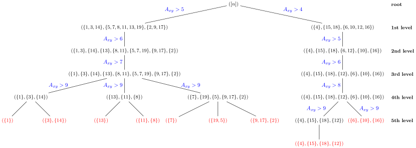
Figure 3: Recursion tree. The weak linear order at each node represent the weak linear order $\psi$ given as input to the recursion node, while the number on the edge between two nodes denotes the minimum value in $A$ set to zero before making a new recursion call. The red weak linear orders are the pruned nodes.

Root node
We set $\psi=(V)$ and invoke Algorithm 4. Then, Algorithm 1 would find two connected components:

$$V_{1}=\{1,2,3,5,7,8,9,11,13,14,17,19\},$$

$$V_{2}=\{4,6,10,12,15,16,18\}.$$

Hence, we can split the problem into two subproblems, where we deal with each connected component independently.

1.0 Connected component $V_{1}$, level 0
The submatrix $A[V_{1}]$ induced by $V_{1}$ is shown below (after shifting the matrix by $a_{\min}=2$, i.e., substracting $2J$ from it).

$$A[V{}_1]=\begin{array}{ccccccccccccc}& 1& 2& 3& 5& 7& 8& 9& 11& 13& 14& 17& 19\\ 1& 9& 0& 7& 3& 3& 3& 0& 3& 3& 4& 0& 3\\ 2& & 9& 0& 7& 6& 3& 8& 3& 3& 0& 8& 6\\ 3& & & 9& 3& 3& 3& 0& 3& 3& 8& 0& 3\\ 5& & & & 9& 6& 5& 7& 5& 5& 3& 7& 8\\ 7& & & & & 9& 5& 6& 5& 5& 3& 6& 7\\ 8& & & & & & 9& 4& 8& 6& 5& 4& 5\\ 9& & & & & & & 9& 4& 3& 0& 8& 6\\ 11& & & & & & & & 9& 7& 5& 4& 5\\ 13& & & & & & & & & 9& 5& 3& 5\\ 14& & & & & & & & & & 9& 0& 3\\ 17& & & & & & & & & & & 9& 6\\ 19& & & & & & & & & & & & 9\end{array}$$ (4)

References

- [1] J.E. Atkins, E.G. Boman, and B. Hendrickson. A spectral algorithm for seriation and the consecutive ones problem. SIAM Journal on Computing, 28:297–310, 1998.
- [2] H.L. Bodlaender, T. Kloks, and R. Niedermeier. SIMPLE MAX-CUT for unit interval graphs and graphs with few s. Electronic Notes in Discrete Mathematics, 3:19–26, 1999.
- [3] K.S. Booth and G.S. Lueker. Testing for the consecutive ones property, interval graphs, and graph planarity using PQ-tree algorithms. Journal of Computer and System Sciences, 13(3):335–379, 1976.
- [4] A. Brandstädt, F.F. Dragan, and F. Nicolai. Lexbfs-orderings and powers of chordal graphs. Discrete Mathematics, 171(1–3):27–42, 1997.
- [5] V. Chepoi and B. Fichet. Recognition of Robinsonian dissimilarities. Journal of Classification, 14(2):311–325, 1997.
- [6] V. Chepoi and M. Seston. Seriation in the presence of errors: A factor 16 approximation algorithm for -fitting Robinson structures to distances. Algorithmica, 59(4):521–568, 2011.
- [7] J. Cohen, F. Fomin, P. Heggernes, D. Kratsch, and G. Kucherov. Optimal linear arrangement of interval graphs. In Mathematical Foundations of Computer Science 2006, volume 4162 of Lecture Notes in Computer Science, pages 267–279. Springer Berlin Heidelberg, 2006.
- [8] D.G. Corneil. A simple 3-sweep LBFS algorithm for the recognition of unit interval graphs. Discrete Applied Mathematics, 138(3):371–379, 2004.
- [9] D.G. Corneil, H. Kim, S. Natarajan, S. Olariu, and A.P. Sprague. Simple linear time recognition of unit interval graphs. Information Processing Letters, 55(2):99–104, 1995.
- [10] D.G. Corneil, S. Olariu, and L. Stewart. The ultimate interval graph recognition algorithm? In Proceedings of the 9th Annual ACM-SIAM Symposium on Discrete Algorithms, SODA ’98, pages 175–180. SIAM, 1998.
- [11] P. Crescenzi, D.G. Corneil, J. Dusart, and M. Habib. New trends for graph search. PRIMA Conference in Shanghai, June 2013. available at http://math.sjtu.edu.cn/conference/Bannai/2013/data/20130629B/slides1.pdf.
- [12] C.M.H de Figueiredo, J.Meidanis, and C.P de Mello. A linear-time algorithm for proper interval graph recognition. Information Processing Letters, 56(3):179–184, 1995.
- [13] X. Deng, P. Hell, and J. Huang. Linear-time representation algorithms for proper circular-arc graphs and proper interval graphs. SIAM Journal on Computing, 25(2):390–403, 1996.
- [14] M. Dom. Algorithmic aspects of the consecutive-ones property. Bulletin of the European Association for Theoretical Computer Science, 98:27––59, 2009.
- [15] F. Fogel, R. Jenatton, F. Bach, and A. d’Aspremont. Convex relaxations for permutation problems. In Advances in Neural Information Processing Systems, pages 1016–1024, 2013.
- [16] D.R. Fulkerson and O.A. Gross. Incidence matrices and interval graphs. Pacific Journal of Mathematics, 15(3):835–855, 1965.
- [17] P.C. Gilmore and A.J. Hoffman. A characterization of comparability graphs and of interval graphs. Canadian Journal of Mathematics, 16:539–548, 1964.
- [18] M.C. Golumbic. Algorithmic graph theory and perfect graphs (Annals of Discrete Mathematics, Vol 57). North-Holland Publishing Co., Amsterdam, The Netherlands, 2004.
- [19] M. Habib, R. McConnell, C. Paul, and L. Viennot. Lex-BFS and partition refinement, with applications to transitive orientation, interval graph recognition and consecutive ones testing. Theoretical Computer Science, 234(1–2):59–84, 2000.
- [20] P. Hell and J. Huang. Certifying LexBFS recognition algorithms for proper interval graphs and proper interval bigraphs. SIAM Journal on Discrete Mathematics, 18(3):554–570, 2005.
- [21] P. Hell, R. Shamir, and R. Sharan. A fully dynamic algorithm for recognizing and representing proper interval graphs. SIAM Journal on Computing, 31(1):289–305, 2002.
- [22] J.Bang-Jensen, J. Huang, and L. Ibarra. Recognizing and representing proper interval graphs in parallel using merging and sorting. Discrete Applied Mathematics, 155(4):442–456, 2007.
- [23] M. Laurent and M. Seminaroti. A Lex-BFS-based recognition algorithm for Robinsonian matrices. In Algorithms and Complexity: Proceedings of the 9th International Conference CIAC 2015, volume 9079 of Lecture Notes in Computer Science, pages 325–338. Springer-Verlag, 2015.
- [24] M. Laurent and M. Seminaroti. The quadratic assignment problem is easy for Robinsonian matrices with Toeplitz structure. Operations Research Letters, 43(1):103–109, 2015.
- [25] I. Liiv. Seriation and matrix reordering methods: An historical overview. Statistical Analysis and Data Mining, 3(2):70–91, 2010.
- [26] P.J. Looges and S. Olariu. Optimal greedy algorithms for indifference graphs. Computers & Mathematics with Applications, 25(7):15–25, 1993.
- [27] R. Mahesh, C.P. Rangan, and A. Srinivasan. On finding the minimum bandwidth of interval graphs. Information and Computation, 95(2):218–224, 1991.
- [28] B.G. Mirkin and S.N. Rodin. Graphs and genes. Biomathematics (Springer-Verlag). Springer, 1984.
- [29] S. Olariu. An optimal greedy heuristic to color interval graphs. Information Processing Letters, 37(1):21–25, 1991.
- [30] P. Préa and D. Fortin. An optimal algorithm to recognize Robinsonian dissimilarities. Journal of Classification, 31:1–35, 2014.
- [31] F.S. Roberts. Indifference graphs. pages 139––146. Academic Press, 1969.
- [32] F.S. Roberts. On the compatibility between a graph and a simple order. Journal of Combinatorial Theory, Series B, 11(1):28–38, 1971.
- [33] F.S. Roberts. Graph theory and its applications to problems of society. Society for Industrial and Applied Mathematics, 1978.
- [34] W.S. Robinson. A method for chronologically ordering archaeological deposits. American Antiquity, 16(4):293–301, 1951.
- [35] D.J Rose and R.E. Tarjan. Algorithmic aspects of vertex elimination. In Proceedings of 7th Annual ACM Symposium on Theory of Computing, STOC ’75, pages 245–254. ACM, 1975.
- [36] M. Seminaroti. Combinatorial Algorithms for the Seriation Problem. PhD thesis, Tilburg University, 2016.
- [37] M. Seston. Dissimilarités de Robinson: algorithmes de reconnaissance et d’approximation. PhD thesis, Université de la Méditerranée, 2008.
- [38] K. Simon. A new simple linear algorithm to recognize interval graphs. In H. Bieri and H. Noltemeier, editors, Computational geometry-methods, algorithms and applications, volume 553 of Lecture Notes in Computer Science, pages 289–308. Springer Berlin Heidelberg, 1991.