Evolution of non-spherical pulsars with plasma-filled magnetospheres

Abstract

Pulsars are famous for their rotational stability. Most of them steadily spin down and display a highly repetitive pulse shape. But some pulsars experience timing irregularities such as nulling, intermittency, mode changing and timing noise. As changes in the pulse shape are often correlated with timing irregularities, precession is a possible cause of these phenomena. Whereas pulsar magnetospheres are filled with plasma, most pulsar precession studies were carried out within the vacuum approximation and neglected the effects of magnetospheric currents and charges. Recent numerical simulations of plasma-filled pulsar magnetospheres provide us with a detailed quantitative description of magnetospheric torques exerted on the pulsar surface. In this paper, we present the study of neutron star evolution using these new torque expressions. We show that they lead to (1) much slower long-term evolution of pulsar parameters and (2) much less extreme solutions for these parameters than the vacuum magnetosphere models. To facilitate the interpretation of observed pulsar timing residuals, we derive an analytic model that (1) describes the time evolution of non-spherical pulsars and (2) translates the observed pulsar timing residuals into the geometrical parameters of the pulsar. We apply this model to two pulsars with very different temporal behaviours. For the pulsar B1828-11, we demonstrate that the timing residual curves allow two pulsar geometries: one with stellar deformation pointing along the magnetic axis and one along the rotational axis. For the Crab pulsar, we use the model show that the recent observation of its magnetic and rotational axes moving away from each other can be explained by precession.

1 Introduction

Studies of pulsar evolution are often performed under the assumption of a spherical neutron star in vacuum. In addition to such idealized studies (Deutsch, 1955), it is now possible to perform more realistic numerical simulations in the limit of a plasma-filled magnetosphere (Contopoulos et al., 1999; Spitkovsky, 2006; Kalapotharakos & Contopoulos, 2009; Tchekhovskoy et al., 2013), and more recently in the full kinetic limit (Philippov & Spitkovsky, 2014; Chen & Beloborodov, 2014; Cerutti et al., 2015; Philippov et al., 2015; Belyaev, 2015). These models predict the evolution of the pulsar rotation period $P$ and the inclination angle $\alpha$ that the magnetic axis makes with the rotational axes. For a spherically-symmetric star, the pulsar period slowly increases and the inclination angle gradually decreases towards $0^{\circ}$ (Philippov et al. 2014; but see Beskin et al. 1993). However, deviations in the pulsar pulse arrival times from the expectations of the above smooth time-evolution, e.g., pulsar timing noise and intermittency, indicate that pulsar spindown may experience quite different, often periodical changes.

One way to introduce an oscillatory behaviour into the spindown is to consider a non-spherical star. In the absence of a physically motivated model of a plasma-filled magnetosphere, previous studies (Goldreich, 1970; Melatos, 2000) considered pulsar evolution in the vacuum approximation. In this paper, we investigate the evolution of non-spherical pulsars whose magnetospheres are filled with plasma. For this, we use recent results of magnetohydrodynamic (MHD) simulations of plasma-filled magnetospheres (Philippov et al., 2014).

The paper is organized as follows. We start with the discussion of the vacuum approximation for pulsar spindown in Section 2. We discuss the parametrisation of magnetospheric torques in Section 3. The solutions for spherical pulsars are presented in Section 4. The effects of stellar non-sphericity are discussed in Section 5. We discuss the implications of our results in Section 6 and conclude in Section 7.

2 Vacuum solution

A pulsar rotating in vacuum emits magnetodipole radiation that carries away the angular momentum of the neutron star. The resulting torque acting on the star could be found by integrating the stresses exerted at its surface,

$$K_{i}=\int\epsilon_{ijk}r_{j}n_{l}T_{kl}{\rm d}S,$$ (1)

where the summation over repeated indices is implied, $T_{kl}$ is the stress tensor (in our case, we have only electromagnetic forces acting on the star, so it is Maxwell’s stress tensor), $\epsilon_{ijk}$ is the Levi-Civita symbol, ${\boldsymbol{r}}$ is the position of surface element with an area element ${\rm d}S$, and $n_{l}$ is the normal vector.

If we know electric and magnetic field components near the stellar surface, it is straightforward to compute the torque $\boldsymbol{K}$ from eq. (1). Deutsch (1955) computed vacuum electromagnetic fields near a rotating spherical star endowed with a dipolar magnetic field. Using these expressions, Michel & Goldwire (1970) derived the torques acting on the pulsar in vacuum. If pulsar’s angular frequency vector ${\boldsymbol{\Omega}}$ is oriented along the $z$-axis and the pulsar magnetic moment vector $\boldsymbol{\mu}$ lies in the $x$ – $z$ plane, the torque components in the vacuum limit are:

$$K_{z} =-\frac{2}{3}K_{\rm aligned}\sin^{2}\alpha,$$ (2)

$$K_{x} =\phantom{-}\frac{2}{3}K_{\rm aligned}\sin\alpha\cos\alpha,$$ (3)

where

$$K_{\rm aligned}=\frac{\mu^{2}\Omega^{3}}{c^{3}}$$ (4)

and $\alpha$ is the inclination angle, i.e., the angle between $\boldsymbol{\Omega}$ and $\boldsymbol{\mu}$.

The torque component due to eq. (2) slows down stellar rotation. The torque component given by eq. (3) points towards $\boldsymbol{\mu}$. Under the action of this torque component, the inclination angle $\alpha$ evolves toward the alignment, and the star approaches the state of minimum angular momentum and energy loss (Philippov et al., 2014).

Though the vacuum magnetosphere model predicts the spindown rate close to the observed value, it has several important shortcomings. The magnetospheres of real pulsars are filled with plasma that inevitably modifies the structure of the magnetic fields via the charges and currents that it carries (Goldreich & Julian, 1969). We discuss these plasma effects below.

3 Magnetospheric torques

Unfortunately, there is no simple analytical solution for magnetospheric torques in the plasma-filled magnetosphere case. Thus, we will rely on the recent advances in numerical simulations of oblique pulsar magnetospheres (Spitkovsky, 2006; Kalapotharakos & Contopoulos, 2009; Tchekhovskoy et al., 2013; Philippov et al., 2015; Tchekhovskoy et al., 2015) that allow us to quantitatively study the influence of magnetospheric charges and currents on the structure of the magnetosphere as well as on the pulsar spindown and alignment.

Philippov et al. (2014) analyzed the results of force-free and MHD simulations and came up with the following parametrization of magnetospheric torques for plasma-filled magnetospheres, to which for simplicity we will refer to below as simply MHD magnetospheres:

$$K_{z} =-K_{\rm aligned}(k_{0}+k_{1}\sin^{2}\alpha),$$ (5)

$$K_{x} =k_{2}K_{\rm aligned}\sin\alpha\cos\alpha,$$ (6)

where $k_{0}$, $k_{1}$ and $k_{2}$ are factors of order unity. They weakly depend on $R_{*}/R_{LC}$, the ratio of the stellar radius $R_{*}$ to the light cylinder radius $R_{LC}=c/\Omega$. Typical parameters for vacuum and MHD models are listed in Table 1 (Philippov et al., 2014).

In addition to torque components (5) and (6), we need to know the anomalous torque, or the torque component directed along ${\boldsymbol{\Omega}}\times{\boldsymbol{\mu}}$, which could be written as

$$K_{y}=k_{3}K_{\rm aligned}\frac{c}{\Omega R}\sin\alpha\cos\alpha,$$ (7)

where $k_{3}={\rm const}$. Melatos (2000) estimated $k_{3}=0.3$. In numerical simulations, anomalous torque is hard to measure as it diverges with $R\rightarrow 0$. We estimate it in our MHD model to be $k_{3}\approx 0.1$ (please see Table 1). As we will show below, the timing residuals do not depend on the strength of the anomalous torque and the value of $k_{3}$ (see Section 5.3).

Table 1: Spindown parameters of different magnetospheric models. $k_{0}$, $k_{1}$ and $k_{2}$ are defined in equations (5) - (6), and $k_{3}$ is referred to the anomalous torque and is defined in equation (7).

Model	$k_{0}$	$k_{1}$	$k_{2}$	$k_{3}$
Vacuum	0	2/3	2/3	$0.3$
MHD/force-free	1	1	1	$\sim 0.1$

The most important difference between vacuum and MHD models is in the value of parameter $k_{0}$, which describes the energy losses of an aligned rotator. In vacuum, an aligned rotator does not spin down, i.e. $\alpha=0$, $\Omega\neq 0$ is a solution to evolution equations. This is impossible in the MHD case, because the spindown luminosity of an aligned rotator is non-zero.

4 Evolution of spherical stars

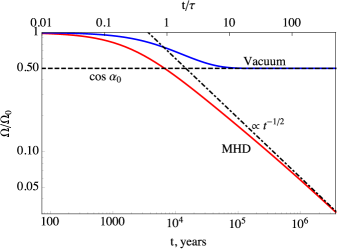
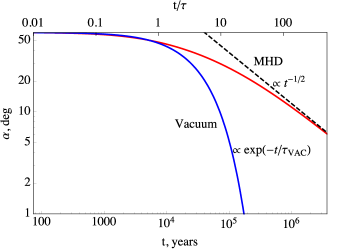
Figure 1: Evolution of a spherical pulsar with initial angle $\alpha_{0}=60$ degrees and angular frequency $\Omega_{0}$. Time on the upper horizontal axis is measured in units of characteristic pulsar spin down time $\tau=Ic^{3}/\mu^{2}\Omega_{0}^{2}$. [Left panel:] The evolution of angular velocity of the neutron star. Vacuum pulsars evolve toward a constant rotational frequency, $\Omega_{0}\cos\alpha_{0}$, while MHD pulsars follow power-law dependence, $\Omega\propto t^{-1/2}$ for $t\gg\tau$. [Right panel:] The evolution of the obliquity angle. In the vacuum case, the evolution is exponentially fast and leads to a very sharp decrease in the inclination angle. In the MHD case, the evolution is a power-law in time, $\alpha\propto t^{-1/2}$.

The torque given by equations (5) – (6) forces the star to change its angular velocity as

$$\text{{{K}}}=I\frac{{\rm d}{\boldsymbol{\Omega}}}{{\rm d}t},$$ (8)

where $I$ is the stellar moment of inertia. The torque component $K_{z}$ acts in the direction opposite to $\boldsymbol{\Omega}$ and reduces the magnitude of angular velocity without changing its direction. On the other hand, $K_{x}$ and $K_{y}$ act perpendicular to $\boldsymbol{\Omega}$ and change its direction without changing its magnitude. $K_{x}$ moves angular velocity towards the magnetic moment $\boldsymbol{\mu}$, so it changes the inclination angle $\alpha$. The anomalous torque component, $K_{y}$, causes the star to precess on the timescale of

$$T_{\rm anom}=2\pi\tau_{\rm anom}=\frac{2\pi IRc^{2}}{\mu^{2}\Omega k_{3}}=\frac{2\pi\xi}{Rc\dot{P}k_{3}},$$ (9)

where the prefactor

$$\xi=k_{0}+k_{1}\sin^{2}\alpha$$ (10)

reflects the inclination-dependence of pulsar radiation losses (see eq. 5). As we will see below, the anomalous torque does not affect the long-term evolution of spherical stars and has only a limited effect on the evolution of non-spherical stars.

A spherical star evolves according to,

$$I\frac{{\rm d}\Omega}{{\rm d}t} =K_{z},$$ (11)

$$I\Omega\frac{{\rm d}\alpha}{{\rm d}t} =-K_{x}.$$ (12)

The solution of pulsar evolution equations could be simplified, because the system of equations (5)–(6) and (11)–(12) has an integral

$$\Omega\left(\frac{\cos^{k_{0}+k_{1}}\alpha}{\sin^{k_{0}}\alpha}\right)^{1/k_{2}}=\Omega_{0}\left(\frac{\cos^{k_{0}+k_{1}}\alpha_{0}}{\sin^{k_{0}}\alpha_{0}}\right)^{1/k_{2}},$$ (13)

which in the case of vacuum losses ($k_{0}=0$, $k_{1}=k_{2}=2/3$, see Tab. 1) reduces to

$$\Omega\cos\alpha=\Omega_{0}\cos\alpha_{0},$$ (14)

and in the MHD case ($k_{0}=k_{1}=k_{2}=1$) to

$$\Omega\frac{\cos^{2}\alpha}{\sin\alpha}=\Omega_{0}\frac{\cos^{2}\alpha_{0}}{\sin\alpha_{0}}.$$ (15)

Most of the works on the pulsar evolution assume magnetodipole (vacuum) radiation and ignore the evolution of the obliquity angle, $\alpha$ (Popov & Turolla, 2012; Igoshev & Popov, 2013). However, as one can show from equations (11)–(12), the inclination angle evolves on the same timescale,

$$\tau=\frac{I\Omega}{K_{\rm aligned}}=\frac{Ic^{3}}{\mu^{2}\Omega^{2}}=\frac{P\xi}{\dot{P}},$$ (16)

as the angular velocity, where $\xi$ is given by eq. (10). Here $P$ and $\dot{P}$ are the pulsar period and period time derivative, respectively.

As pulsars spin down, the obliquity angle evolves and this affects the spindown. Therefore, it is crucial to account for the change in $\alpha$. For instance, if we do not account for the alignment effect in the vacuum case, i.e. postulate $\alpha=$ constant, a pulsar starting out with $\Omega=\Omega_{0}$ and $\alpha=\alpha_{0}$ evolves towards $\Omega_{\rm final}=0$. However, the correct solution of eqs. (11)–(12) with torques given by eqs. (5)–(6) yields $\Omega_{\rm final}=\Omega_{0}\cos\alpha_{0}$, which is comparable to $\Omega_{0}$ for representative $\alpha_{0}\sim 60^{\circ}$.

Though both vacuum and MHD models evolve toward the aligned configuration, they approach it through quite different paths. The inclination angle of a vacuum pulsar evolves according to

$$\sin\alpha=\sin\alpha_{0}\exp\left(-t/\tau^{\rm VAC}_{\rm align}\right),$$ (17)

where $\tau_{\rm align}^{\rm VAC}=1.5\tau\cos^{-2}\alpha_{0}$, and $\tau$ is pulsar spindown timescale given by eq. (16). Thus, the vacuum pulsar evolves to the aligned configuration exponentially fast, without a significant slowdown of its rotation. For an MHD pulsar, we have the following implicit solution,

$$\frac{1}{2\sin^{2}\alpha}+\log(\sin\alpha)=\frac{t}{\tau_{\rm align}^{\rm MHD}}+\frac{1}{2\sin^{2}\alpha_{0}}+\log(\sin\alpha_{0}),$$ (18)

where $\tau_{\rm align}^{\rm MHD}=\tau\sin^{2}\alpha_{0}/\cos^{4}\alpha_{0}$, which asymptotes at late times to a power-law, $\alpha\propto t^{-1/2}$ (Philippov et al., 2014).

Figure 1 illustrates the evolution under vacuum and MHD torques of a spherical pulsar with an initial angle of $\alpha_{0}=60$ degrees and Crab-like parameters, $P=0.033$ s, $B=3.78\times 10^{12}\ {\rm G}$, $\tau=7.4\times 10^{3}$ years. One can see that for a vacuum pulsar the inclination angle becomes exponentially small just after $t\geq\tau^{\rm VAC}_{\rm align}$ which equals to $6\tau$ for Crab’s parameters. On the other hand, the obliquity angle in the MHD case changes only by a factor of few for the same parameters. Note also that MHD pulsars lose angular momentum more efficiently than vacuum ones. Instead of pulsar rotation asymptoting to $\Omega_{\rm final}=\Omega_{0}\cos\alpha_{0}$ as for vacuum pulsars, MHD pulsars lose a substantial amount of angular momentum during its lifetime, and $\Omega$ continuously decreases, asymptotically approaching zero: $\Omega\propto t^{-1/2}$. Characteristic timescale of pulsar spindown is around $10^{4}{-}10^{5}$ years (i.e. the timescale over which $\Omega$ changes by a factor of 2).

5 Evolution of non-spherical stars

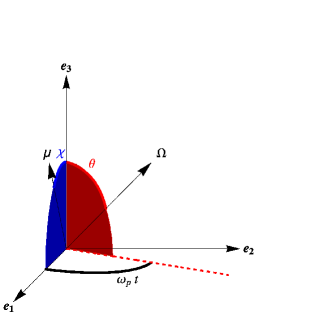
Figure 2: In this work, we use the following coordinate system: $\boldsymbol{e}_{1}$, $\boldsymbol{e}_{2}$, $\boldsymbol{e}_{3}$ denote the principal axes of the star, which is characterised by a stellar magnetic moment $\boldsymbol{\mu}$ and angular frequency $\boldsymbol{\Omega}$. Pulsar geometry is defined by several angles: $\chi$ between $\boldsymbol{\mu}$ and $\boldsymbol{e}_{3}$, $\theta$ between $\boldsymbol{\Omega}$ and $\boldsymbol{e}_{3}$, and $\alpha$ (not shown) between $\boldsymbol{\mu}$ and $\boldsymbol{\Omega}$. During free precession, $\boldsymbol{\Omega}$ rotates around $\boldsymbol{e}_{3}$ and the angle between the $\boldsymbol{e}_{1}$ and the projection of $\boldsymbol{\Omega}$ on $\boldsymbol{e}_{1}$-$\boldsymbol{e}_{2}$ plane increases at a constant rate $\omega_{p}$.

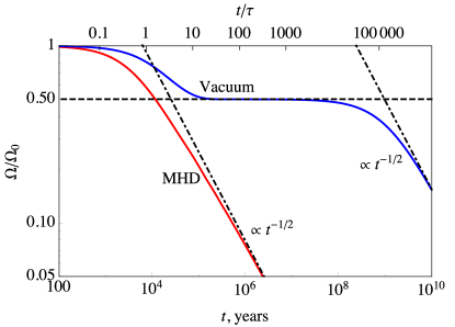
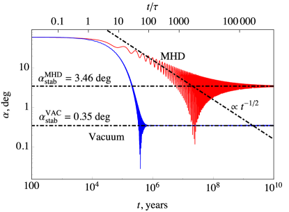
Figure 3: The time evolution of a non-spherical pulsar with the initial inclination angle $\alpha_{0}=60$ deg, angles $\theta_{0}=60$ deg and $\chi_{0}=1$ deg (see Fig. 2 for the angle definitions), ellipticity $\varepsilon=1.66\times 10^{-13}$, and angular frequency $\Omega_{0}$. [Left panel:] The angular velocity $\Omega$ vs time. Despite the star is non-spherical, $\Omega$ evolves in a very similar way to the spherical case. [Right panel:] The inclination angle $\alpha$ vs time. The stellar non-sphericity causes $\alpha$ to oscillate at late time, $t\gtrsim 10\tau$ in both vacuum and MHD cases. Despite that, in a time-average sense the inclination angle undergoes a secular decrease. Eventually, the inclination angle stabilises. The stabilisation in MHD pulsars occurs at a much later time than in vacuum pulsars.

The rotation of pulsars steadily slows down, and the radio pulse profile is mostly stable in time. The deviation from smooth spindown is often less than one part in $10^{11}$, but at this accuracy pulsars experience rather random irregularities, which are referred to as timing noise.

Lyne et al. (2010) presented timing residuals (deviations from steady spindown) of 17 pulsars that showed a quasi-periodic behaviour. The characteristic period of these variations is a few hundred days, hence prolonged observations are needed to investigate this behaviour. Interestingly, a lot of pulsars with timing noise exhibit variations in the pulse profile that are correlated with variations in the period. This makes a change in geometry (e.g., precession-induced changes in the inclination angle) a possible explanation of this phenomenon. Below we focus on the two cases of pulsar B1828-11 and the Crab pulsar. In this section, we set $R=10^{6}$ cm and consider the case of a plasma-filled magnetosphere, i.e., set $k_{0}=k_{1}=k_{2}=1$.

Previously, we discussed a spherical star with an isotropic tensor of inertia. Generally, a rigid star has a triaxial inertia tensor that is diagonalised in the basis of its principal axes. Let us denote the pulsar principal axes as $\boldsymbol{e}_{1}$, $\boldsymbol{e}_{2}$, $\boldsymbol{e}_{3}$ and corresponding moments of inertia as $I_{1}=I$, $I_{2}=I(1+\varepsilon_{12})$ and $I_{3}=I(1+\varepsilon_{13})$, respectively. Here, $\varepsilon_{12}$ and $\varepsilon_{13}$ characterise the degree of stellar non-sphericity.

We will start with the case of a biaxial star, i.e., we will set $\varepsilon_{12}=0$, $\varepsilon_{13}=\varepsilon\neq 0$. Without the loss of generality, we choose $\boldsymbol{e}_{1}$ to lie in the $\boldsymbol{e}_{3}{-}\boldsymbol{\mu}$ plane. As seen in Fig. 2, the problem geometry is now set by three angles: angle $\chi$ between $\boldsymbol{\mu}$ and $\boldsymbol{e}_{3}$, angle $\theta$ between $\boldsymbol{\Omega}$ and $\boldsymbol{e}_{3}$ and angle $\alpha$ between $\boldsymbol{\Omega}$ and $\boldsymbol{\mu}$. Note that the values of these angles are not completely arbitrary but are constrained by $|\theta-\chi|\leq\alpha\leq|\theta+\chi|$. Here and below, indices ($1$, $2$, $3$) refer to the coordinate system set by the principal axes and ($x$, $y$, $z$) to the coordinate system described in Section 2.

For a non-spherical pulsar, instead of equations (11)–(12) we need to solve Euler’s equations of motion of a rigid body:

$$\dot{L}_{i}=\epsilon_{ijk}L_{j}\Omega_{k}+K_{i},$$ (19)

where summation over repeated indices is implied, $K_{i}$ and $\Omega_{i}$ are the components of $\boldsymbol{K}$ and $\boldsymbol{\Omega}$ in the ($\boldsymbol{e}_{1}$, $\boldsymbol{e}_{2}$, $\boldsymbol{e}_{3}$) coordinate system and $L_{i}=I_{i}\Omega_{i}$.

To compute $K_{i}$, we need to make a coordinate transformation from ($\boldsymbol{x}$, $\boldsymbol{y}$, $\boldsymbol{z}$) to ($\boldsymbol{e}_{1}$, $\boldsymbol{e}_{2}$, $\boldsymbol{e}_{3}$). This transformation could be found in Melatos (2000), and we do not give it here. Rewriting equation (19) in the new coordinates, we obtain:

$$\dot{\Omega}_{1}+\varepsilon\Omega_{2}\Omega_{3}=K_{1}/I,$$ (20)

$$\dot{\Omega}_{2}-\varepsilon\Omega_{3}\Omega_{1}=K_{2}/I,$$ (21)

$$(1+\varepsilon)\dot{\Omega}_{3}=K_{3}/I.$$ (22)

We solve these equations numerically using the three angles $\theta_{0}$, $\chi_{0}$ and $\alpha_{0}$ and the initial period $P_{0}$ as the initial conditions. We adopt the following fiducial parameters for a neutron star: mass $M=1.4M_{\sun}$, radius $R=10$ km, dipole moment $\mu=0.5BR^{3}$, and $B=10^{12}$ G.

To see how a small stellar non-sphericity can affect the evolution of a neutron star, let us again consider a Crab-like pulsar, $\alpha_{0}=60^{\circ}$, $P=0.033$ s, $B_{12}=3.78$, $\tau=7.4\times 10^{3}$ years. Fig. 3 shows how this pulsar evolves for $\theta_{0}=60^{\circ}$, $\chi_{0}=1^{\circ}$ and $\varepsilon=1.66\times 10^{-13}$. The right panel in Fig. 3 shows that even such a seemingly small ellipticity causes the inclination angle $\alpha$ to vary with a substantial amplitude. These variations are due to the free precession of the star, at the period set by the degree of stellar non-sphericity:

$$T_{\rm prec}=2\pi\tau_{\rm prec}=\frac{P}{\varepsilon},$$ (23)

which for our choice of parameters is $T_{\rm prec}=6300~{}{\rm years}$. As we will see below, the standard expression (23) applies only in the limit of angular frequency pointing along the symmetry axis of the neutron star, $\boldsymbol{e}_{3}$, i.e., for $\cos\theta_{0}\approx 1$ [see equation (48), which generalises eq. (23) to other values of $\theta_{0}$].

In vacuum, the rotation of a spherical star asymptotes to a non-zero value: this is because pulsars quickly evolve toward the alignment $\alpha=0$ and their spindown torque vanishes. In contrast, the left panel in Fig. 3 shows that non-spherical vacuum pulsar rotation slows down all the way to zero. This is because non-sphericity effects cause the inclination angle to stabilise at a finite value, e.g., at $\alpha_{\rm stab}^{\rm VAC}=0.35$ deg for our choice of pulsar parameters, which prevents the spindown torque from vanishing (see eq. 2). Similarly, for MHD pulsars, stellar non-sphericity leads to the inclination angle stabilisation at a finite value, e.g., at $\alpha^{\rm MHD}_{\rm stab}=3.46^{\circ}$ for our choice of pulsar parameters, as seen in the right panel of Fig. 3. The value of the stabilisation angle depends on the strength of anomalous torque and the $k_{3}$ factor (see Tab. 1) and can substantially differ between vacuum and MHD models; a study of this dependence is beyond the scope of this work.

After stabilisation, the evolution of the angular velocity of the neutron star can be approximated by

$$\langle\dot{\Omega}\rangle=-\frac{\langle\Omega\rangle^{3}\mu^{2}}{Ic^{3}}(k_{0}+k_{1}\sin^{2}\alpha_{\rm stab}),$$ (24)

where brackets $\langle\dots\rangle$ denote the averaging over a precession period. Equation (24) has a solution

$$\frac{1}{\langle\Omega\rangle^{2}}-\frac{1}{\Omega_{\rm stab}^{2}}=\frac{t}{\tau_{\rm evol}},$$ (25)

where $\tau_{\rm evol}$ is the characteristic timescale of evolution and $\Omega_{\rm stab}$ is the value of angular frequency at stabilisation. The timescale $\tau_{\rm evol}$ is determined by the stabilisation angle and is different in vacuum and MHD cases:

$$\tau_{\rm evol}^{\rm VAC} =1.5\tau\sin^{-2}\alpha_{\rm stab}\gg\tau,$$ (26)

$$\tau_{\rm evol}^{\rm MHD} =\tau(1+\sin^{2}\alpha_{\rm stab})^{-1}\approx\tau.$$ (27)

Equation (25) implies a plateau in $\langle\Omega\rangle$ at early times post-stabilisation (see the left panel of Fig. 3) and a power-law evolution at late times, $t\gtrsim\tau_{\rm evol}$. For the case shown in Figure 3 the analytical estimate (26) gives $\tau_{\rm evol}^{\rm VAC}=5.21\times 10^{8}$ years, in agreement with the end of plateau.

Figure 3 shows that until the inclination angle stabilises, the solution for a non-spherical pulsar is similar to the solution for a spherically-symmetric neutron star, except for small-amplitude short timescale oscillations super-imposed on top of the secular alignment trend. This allows us make use of eqs. (17) and (18) to obtain a simple estimate of the time at which the stabilisation sets in:

$$t_{\rm stab}^{\rm VAC} =1.5\tau\frac{\log(\sin\alpha_{0}/\sin\alpha_{\rm stab})}{\cos^{2}\alpha_{0}}\sim{\rm few}\times\tau,$$ (28)

$$t_{\rm stab}^{\rm MHD} \approx\frac{\tau}{\alpha_{\rm stab}^{2}}.$$ (29)

Here we assumed the stabilisation angle to be small and neglected the logarithmic factor in eq. (28). Importantly, the stabilisation time for MHD pulsars is much larger than for vacuum ones:

$$\frac{t_{\rm stab}^{\rm MHD}}{t_{\rm stab}^{\rm VAC}}\sim\frac{1}{{\rm few}\times\alpha_{\rm stab}^{2}}\gg 1,$$ (30)

but even for the vacuum pulsar this is a large timescale: for the initial conditions used in Fig. 3, $t_{\rm stab}^{\rm VAC}\sim 10^{5}$ years. For MHD pulsars it is $\gtrsim 10^{8}$ years (for $\alpha_{\rm stab}\lesssim 0.03$). We thus expect that pulsars cross the death line before their inclination angle has a chance to reach a small value and become stabilised.

5.1 Neutron Star Ellipticities

Due to the uncertainties in the neutron star equation of state (Glendenning, 1997), it is hard to estimate how much the pulsar crust is deformed and therefore to theoretically compute the value of ellipticity. Horowitz & Kadau (2009) performed multi-million ion molecular dynamics simulations showing that the neutron star crust can support ellipticities up to $\epsilon_{\rm max}=4\times 10^{-6}$. This ellipticity corresponds to a precession time of a few days for a one-second pulsar (see eq. 23).

There are two main contributors to the neutron star ellipticity: fast rotation and strong magnetic fields in the interior. The non-sphericity caused by rotation can be estimated as the ratio between its rotational and gravitational energies:

$$\varepsilon_{\rm rot}=\frac{E_{\rm rot}}{E_{\rm grav}}\approx 7\times 10^{-8}P_{1}^{-2}R_{6}^{3}M_{1.4}^{-1},$$ (31)

where $R=R_{6}\times 10^{6}$ cm, $P=P_{1}\times 1$ s, and $M=M_{1.4}\times 1.4M_{\odot}$. This deformation is pointed along the rotational axis.

However, not the entirety of this ellipticity participates in precession. The neutron star supports hydrostatic stresses only after the crystallisation of its crust. The part of the ellipticity that participates in precession is much smaller than the value given by eq. (31) and can be written as (see, e.g., Munk & MacDonald, 1975):

$$\varepsilon_{\rm cr}=\frac{\tilde{\mu}}{1+\tilde{\mu}}\varepsilon_{\rm rot}=2\times 10^{-11}\mu_{30}P^{-2}R_{6}^{7}M_{1.4}^{-3},$$ (32)

where $\tilde{\mu}=19\mu^{\rm cr}/2\rho gR$, where $g$ is the surface gravity, $\rho$ is the density and $\mu^{\rm cr}$ is shear modulus of the crust, whose fiducial value is $10^{30}\ {\rm dyn\;cm^{-2}}$.

The impact of the magnetic field can be calculated in a similar way:

$$\varepsilon_{\rm mag}=\frac{E_{\rm mag}}{E_{\rm grav}}\approx 10^{-12}B_{12}^{2}R_{6}^{4}M_{1.4}^{-2},$$ (33)

where $B=B_{12}\times 10^{12}\ {\rm G}$. This deformation is pointed along the magnetic moment. We discuss the possible origin of stellar non-sphericity in Section 6.

5.2 Pulsar B1828-11

Pulsar B1828-11 was the first to show highly periodic long-term variations in timing residuals that are correlated with variations in the pulse profile. The spectrum of timing residuals consists of three harmonics with periods 1000, 500 and 250 days. If the period of free precession $P/\varepsilon$ (see eq. 23) equals the largest period in spectrum, ellipticity equals $\varepsilon\approx 4.69\times 10^{-9}$.

We will use the following timing parameters for pulsar B1828-11: $P^{0}=0.405$ s, $\dot{P}_{-15}^{0}=60$. The values with the superscript ‘0’ denote the best fit parameters, and the values without this superscript denote the observations. The characteristic timescales of the pulsar evolution are:

$$\tau =6.75\times 10^{12}\xi~{}{\rm s}$$ (34)

$$\tau_{\rm anom} =3.49\times 10^{9}\xi k_{3}^{-1}~{}{\rm s},$$ (35)

where $\tau$ is spindown timescale given by eq. (16) and $\xi=1+\sin^{2}\alpha$ is a number between $1$ and $2$ that reflects the dependence of MHD pulsar spindown on the inclination angle (see eq. 5).

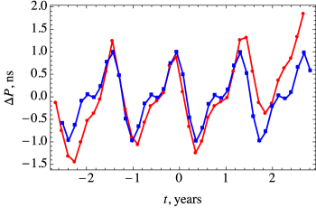
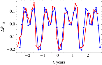
Figure 4: Numerical solution of Euler’s equations (blue squares) giving our best-fit for PSR B1828-11, $\chi=89$ deg, $\theta=6$ deg, and the observed residuals (red dots). [Left panel:] Period residual. The numerical solution is in good agreement with observations, reproducing both the characteristic period and the amplitude. [Right panel:] Period derivative residual. Our numerical solution reproduces the two-bump structure well.

This pulsar also has a well-measured second period derivative $\ddot{P}^{0}=-1.70\times 10^{-25}s^{-1}$ and the changes in the pulse profile are correlated with the changes in $P$ and $\dot{P}$. As seen in Fig. 4, the period timing residual, $\Delta P=P-P^{0}-\dot{P}^{0}t-\ddot{P}^{0}t^{2}/2$, is periodic and has an amplitude of 1.65 ns, and the residual for the period derivative, $\Delta\dot{P}=\dot{P}-\dot{P}^{0}-\ddot{P}^{0}t$, is also periodic and has a magnitude of about $0.19\times 10^{-15}$. In order to compare the outcome of our models to the observations, i.e., compare the simulated values of $\Delta P$ and $\Delta\dot{P}$ to the observations in Fig. 4, we will use the same procedure as was used to determine the observed values of residuals (Lyne et al., 2013): every 50 days (indicated by dots in the figure), we average the residual over the time interval of 100 days.

Stairs et al. (2000) concluded that the most probable explanation for these variations is the precession of the neutron star. Link & Epstein (2001) presented a calculation, where they attempted to find the best-fitting pulsar geometry under the vacuum approximation, that matches the residuals, $\Delta P$, and the changes in the emission profile. We now look for a solution under a more realistic assumption of the plasma-filled magnetosphere.

To reproduce the observational data for pulsar B1828-11, we set $\tau_{\rm prec}=\pm 0.218$ years. The timescale can formally be negative because of the negativity of $\varepsilon$; for the comparison of time scales, what matters is its absolute value, which corresponds to the period of variation of about $500$ days – the leading harmonic in the spectrum – and $\varepsilon=\pm 9.44\times 10^{-9}$. One can also show that for a biaxial star, the timing residuals do not depend on the sign of the ellipticity.

We numerically solve equations (20)–(22) for different initial values of $\alpha$, $\theta$ and $\chi$. After that, we find the mean value of the period and its first two derivatives, and compute the residuals:

$$\delta P =P-\langle P\rangle-\langle\dot{P}\rangle t-\langle\ddot{P}\rangle t^{2}/2,$$ (36)

$$\delta\dot{P} =\dot{P}-\langle\dot{P}\rangle-\langle\ddot{P}\rangle t.$$ (37)

Angles $\theta$, $\chi$ and $\alpha$ are set to their initial values (which are denoted with the subscript ‘0’) at time $t=0$ that corresponds to 50,300 MJD. Euler’s equations are solved in $t$ from $-3$ years to $3$ years to mimic the observed data range. The mean values are calculated over the entire time range.

Table 2: Pulsar B1828-11: Best fit parameters obtained by fitting the pulsar timing residuals (see Fig. 4).

Case	$\theta$, deg	$\chi$, deg	$\varepsilon_{13}$
large $\chi$	5	89	$9.4\times 10^{-9}$
small $\chi$	89	5	$5.4\times 10^{-7}$

Our best fit gives $\chi=89$ deg and $\theta=6$ deg and is presented in Fig. 4 and in Table 2. The solution implies that the evolution of a neutron star is close to free precession with small perturbations caused by the magnetospheric torque. Inclination angle $\alpha$ varies from $\chi-\theta=83$ deg to $\chi+\theta=95$ deg and its initial value simply sets the initial phase of the evolution. As we will discuss below, a symmetry exists between the values of $\theta$ and $\chi$. This symmetry implies the existence of a “mirror” solution with the values of $\theta$ and $\chi$ swapped (see Table 2). To distinguish between these two solutions, we refer to them as the “large $\chi$” and “small $\chi$” solutions. For brevity, we do not show the small $\chi$ solution in Figure 4.

In order to reproduce the magnitude of the observed residuals, in our numerical solution we need to choose the angle $\theta$ to be small and the angle $\chi$ large, or vice versa: as we discuss below, this is required for the residuals to have such a small amplitude as observed, as well as the two-peak structure of the $\dot{P}$ residual.

5.3 Analytical solution for B1828-11

Our numerical solution for pulsar B1828-11 implies that the motion of a slightly non-spherical neutron star is essentially a free precession with a small perturbation caused by the magnetospheric torques.

5.3.1 Free precession

For freely precessing body, Euler’s equations of motion take the following form:

$$\dot{\boldsymbol{L}}+{\boldsymbol{\Omega}}\times\boldsymbol{L}=0.$$ (38)

These equations can be solved analytically in terms of Jacobian elliptic functions $\rm cn,~{}sn~{}and~{}dn$ (Landau & Lifshitz, 1976):

$$L_{1}/I\Omega_{0} =\sin\theta_{0}\;{\rm cn}(\omega_{\rm p}t,k\tan^{2}\theta_{0}),$$ (39)

$$L_{2}/I\Omega_{0} =\sin\theta_{0}(1+k)^{1/2}\;{\rm sn}(\omega_{\rm p}t,k\tan^{2}\theta_{0}),$$ (40)

$$L_{3}/I\Omega_{0} =\cos\theta_{0}\;{\rm dn}(\omega_{\rm p}t,k\tan^{2}\theta_{0}),$$ (41)

where

$$k=\frac{I_{3}(I_{2}-I_{1})}{I_{1}(I_{3}-I_{2})}=\frac{\varepsilon_{12}(1+\varepsilon_{13})}{\varepsilon_{13}-\varepsilon_{12}}\approx\frac{\varepsilon_{12}}{\varepsilon_{13}-\varepsilon_{12}}$$ (42)

and

$$\omega_{\rm p}=\frac{\varepsilon_{13}L\cos\theta_{0}}{I_{3}(1+k)^{1/2}}\approx\frac{\varepsilon_{13}\Omega_{0}\cos\theta}{(1+k)^{1/2}}.$$ (43)

The precession period is equal

$$T_{\rm prec}=\frac{P}{\varepsilon_{13}\cos\theta_{0}}\frac{2F(\pi/2,k\tan^{2}\theta_{0})}{\pi},$$ (44)

where $F(\phi,m)$ is the Legendre elliptic integral of the first kind.

In the case of $\varepsilon_{12}=0$, that is of an axisymmetric star, the solution takes a much simpler form:

$$L_{1}/I\Omega_{0} =\sin\theta_{0}\cos(\omega_{\rm p}t),$$ (45)

$$L_{2}/I\Omega_{0} =\sin\theta_{0}\sin(\omega_{\rm p}t),$$ (46)

$$L_{3}/I\Omega_{0} =\cos\theta_{0},$$ (47)

where $\omega_{\rm p}=\varepsilon_{13}\Omega_{0}\cos\theta_{0}$ and $\Omega_{0}$ is the initial rotational frequency. In this case, the precession period is simply

$$T_{\rm prec}=\frac{P}{\varepsilon_{13}\cos\theta_{0}}.\quad{\rm(biaxial\ star)}$$ (48)

Now we have an exact solution $\boldsymbol{\Omega}_{0}(t)$ for free precession and can use perturbation theory to find the solution for a nonzero magnetospheric torque.

5.3.2 Full perturbative solution for a biaxial star

We find the exact solution for the equation

$$\dot{\boldsymbol{L}}+{\boldsymbol{\Omega}}\times\boldsymbol{L}=\boldsymbol{K}\left[\boldsymbol{\Omega}_{0}(t)\right].$$ (49)

in Appendix A. Here we summarise the most important results.

For an axisymmetric (biaxial) MHD pulsar, the residual in $\dot{P}$ takes the following form (see Appendix A.4 for a derivation):

$$\delta\dot{P}=-\dot{P}^{\rm obs}f(\theta_{0},\chi)[\cos\omega_{\rm p}t+g(\theta_{0},\chi)\cos 2\omega_{\rm p}t]$$ (50)

where $\dot{P}^{\rm obs}$ is the observed value of $\dot{P}$ and

$$f(\theta,\chi) =\frac{\sin 2\theta\sin 2\chi}{4-2\cos^{2}\theta\cos^{2}\chi-\sin^{2}\theta\sin^{2}\chi},$$ (51)

$$g(\theta,\chi) =\tan\theta\tan\chi/4.$$ (52)

The amplitude of the residual is proportional to $\sin 2\theta\sin 2\chi$, and the residual does not depend on the anomalous torque. If we have residuals that are much smaller than $\dot{P}^{\rm obs}$ (which is usually the case), the best-fit values of $\theta$ and $\chi$ are pushed close either to $0$ or to $90$ deg. As the observed residuals for B1828-11 are much smaller than $\dot{P}^{\rm obs}$ and we observe the two-hump structure (and thus have $g(\theta,\chi)\approx 1$), one of the angles is close to 0, and the other one close to 90 deg.

One can see that expressions (51) and (52) are symmetric in respect to the substitution $\theta\leftrightarrow\chi$. This means that we cannot distinguish between the cases of small $\theta$ and small $\chi$, which, as we mentioned previously, we refer to as the cases of large $\chi$ and small $\chi$, respectively. For small $\theta$, the stellar deformation points in the direction of stellar rotation and it is natural to assume that it is caused by rotation. If so, it should be on the order of the analytic expectation, $\varepsilon_{\rm cr}$ (eq. 32). On the other hand, for small $\chi$ it is natural to assume that the deformation is caused by the magnetic field. If so, we would expect the ellipticity to be on the order of $\varepsilon_{\rm mag}$ (eq. 33).

The special case of a biaxial star corresponds to $k=0$ (see eq. 42). For $k=0$ and a small $\theta$ value, we have $\cos\theta\sim 1$ and $T_{\rm prec}=P/\varepsilon$ (see eq. 48). This implies $\varepsilon=9.4\times 10^{-9}$. For $k=0$ and small $\chi$, we find $\cos\theta\sim(\pi/2-\theta)$ and $T_{\rm prec}=P/\varepsilon(\pi/2-\theta)$. For $\theta=89$ deg, this implies $\varepsilon=5.4\times 10^{-7}$. These results are summarised in Tab. 2. We discuss the possible origin of the ellipticity in Sec. 6. Note that for our numerical solution shown in Fig. 4 we chose a small $\theta$ and large $\chi$. For brevity, we do not show the opposite case.

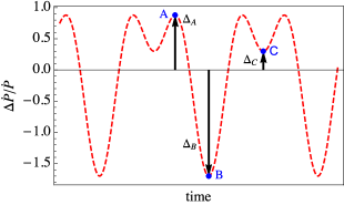
Figure 5: Method of obtaining geometrical parameters of precessing neutron stars from the observations. One needs to measure the residual values at three extremum points ($\Delta_{\rm A}$, $\Delta_{\rm B}$, $\Delta_{\rm C}$) and then calculate $f(\chi,\theta)$ and $g(\chi,\theta)$ using equations (53)-(55). After that, $\chi$ and $\theta$ are implicitly set by the values of $f$ and $g$.

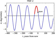
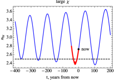
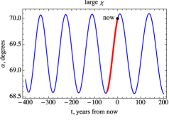
Figure 6: Blue line shows our best-fit numerical solution of Euler’s equations for the Crab pulsar in the large $\chi$ case is shown (see Fig. 7 for the small $\chi$ case). This red line indicates the time range over which timing residuals have been observed and the black dot indicates the present time. Black dashed lines show the observationally-inferred values. The pulsar parameters at $t=0$ are: $\alpha_{0}=70^{\circ}$, $\theta_{0}=2^{\circ}$, $\chi_{0}=68.05^{\circ}$. [Left panel:] The rate of change of the inclination angle, $\dot{\alpha}$. The solution shows an order of magnitude agreement with observations. [Central panel:] The braking index $n_{\rm br}$ vs time. [Right panel:] The inclination angle $\alpha$ vs time. Over the observed time range, $\alpha$ increases almost linearly with time, in agreement with observations.

Using the analytic model we have developed, we now can estimate directly from the observations the values of angles $\theta$ and $\chi$, or, equivalently, the values of the functions $f(\theta,\chi)$ and $g(\theta,\chi)$ (see eqs. 51 and 52). For this, we only needs to measure the following three extremum points, as shown in Fig. 5: the global maximum $\Delta_{\rm A}$ and minimum $\Delta_{\rm B}$ as well as the local minimum $\Delta_{\rm C}$ of the residual,

$$\Delta_{\rm A} = f(\theta_{0},\chi)\left[g(\theta_{0},\chi)+\frac{1}{8g(\theta_{0},\chi)}\right],$$ (53)

$$\Delta_{\rm B} = -f(\theta_{0},\chi)[1+g(\theta_{0},\chi)],$$ (54)

$$\Delta_{\rm C} = f(\theta_{0},\chi)[1-g(\theta_{0},\chi)],$$ (55)

invert these to obtain the values of $f$ and $g$. Note that this system of equations is over-constrained, and this offers a self-consistency check.

5.3.3 Full perturbative solution for a triaxial star

If the star is not axisymmetric, the solution has a much more complex form (but still does not depend of the anomalous torque, see Appendix A.5 for a derivation):

$$\delta\dot{P}=-\dot{P}^{\rm obs}f(\theta_{0},\chi)\mathcal{P}(\theta_{0},\chi,t)$$ (56)

with

$$\mathcal{P} ={\rm cn}(\omega_{p}t){\rm dn}(\omega_{p}t)+{\rm cn}(2\omega_{p}t)\frac{2g(\theta_{0},\chi)}{(1+{\rm dn}(2\omega_{p}t))}+$$ (57)

$$+({\rm dn}(2\omega_{p}t)-1)\left(\frac{g(\theta_{0},\chi)}{(1+{\rm dn}(2\omega_{p}t))}+\frac{g(\theta_{0},\chi)^{-1}}{8(1+{\rm cn}(2\omega_{p}t))}\right).$$

Here we for simplicity do not write the second argument of Jacobian elliptic functions which always equals $k\tan^{2}\theta_{0}$. The second ellipticity does not qualitatively change the behaviour of solution and only influences the precession period (see eq. 44).

5.4 Crab pulsar

The emission from the Crab pulsar (pulsar B0531+21) was observed since 1969 in radio, optical, x-ray and gamma-ray wavebands. The radio pulse profile of this pulsar consists of two components separated by $145^{\circ}$ in phase: the main pulse and the interpulse. During high-precision daily observations performed since year 1991 at Jodrell Bank Observatory, Lyne et al. (2013) found a steady increase in separation between the main pulse and the interpulse, at $0.62^{\circ}\pm 0.03^{\circ}$ per century.

Because radio and gamma-ray pulses of the Crab pulsar arrive at the same pulse phase, it is thought that the radio emission from the Crab pulsar comes from the same magnetospheric region as the gamma-ray emission. Using this fact, as well as gamma-ray emission models, Lyne et al. (2013) concluded that the increase in the separation between the main pulse and the interpulse indicates an increase of the inclination angle at approximately the same rate. The increase of the inclination angle also naturally leads to a braking index value less than 3, in agreement with observations. However, for a spherically symmetric star, MHD models predict a decrease of the inclination angle for a spherical star (see Sect. 4), and a braking index that is always larger than 3. Philippov et al. (2014) suggested that the observed increase of the inclination angle could be due to the precession of the neutron star caused by stellar non-sphericity.

Later, Lyne et al. (2015) revealed the observational data for the Crab pulsar over a 45-year time range. Although the timing residuals show some oscillatory behaviour, they are corrupted by a large number of glitches. This makes it impossible to get an accurate precession model fit. Nevertheless, between the subsequent glitches Crab pulsar behaves as if it were precessing.

The observed increase in the inclination angle of the Crab pulsar can be explained with a precession model. Just as for PSR B1828-11, the timing residuals residuals in $P$ and $\dot{P}$ (Lyne et al., 2015) imply that either $\theta\approx 0$ and $\chi\approx 90$ deg or $\chi\approx 0$ and $\theta\approx 90$ deg.

Table 3: Crab pulsar: Best fit parameters for large and small $\chi$ cases. The second and third frequency derivatives agree with observations to within an order of magnitude, as expected given the large number of Crab’s glitches. The best-fit values of the inclination angle $\alpha$ are agreement with independent estimates (Lyne et al., 2013). Our solution implies a precession period of about $100$ years. Deviations from the near-linear increase in time of the inclination angle could be observed on shorter timescales, perhaps as short as $\sim 20$ years.

Case	$\theta$, deg	$\chi$, deg	$\alpha$, deg	$T_{\rm prec}$, years	$\varepsilon$	$\ddot{\nu},~{}10^{-20}$ Hz/s2	$\dddot{\nu},~{}10^{-30}$ Hz/s3
observations	-	-	-	-	-	1.12	-2.73
large $\chi$	2	68.05	70	126.7	$8.3\times 10^{-12}$	1.15	-0.8
small $\chi$	59.1	1	60	108.5	$1.11\times 10^{-11}$	1.27	0.8

Figure 6 shows our best fit obtained for large $\chi$ case and $\alpha=70^{\circ}$. One can see that for the past 45 years the inclination of the Crab pulsar has increased almost linearly. On larger timescale, the inclination angle is oscillating and its mean value is almost constant. Our fit produces values of $\dot{\nu}$, $\ddot{\nu}$ and $\dddot{\nu}$ close to the observed values. We summarise the inferred pulsar geometry in Table 3. The precession period in this solution is roughly $T_{\rm prec}=126$ years, but there is a strong degeneracy between values of $\theta$ and $T_{\rm prec}$. Making precession period $T_{\rm prec}$ larger (which is allowed by the data) and the wobble angle smaller, one could obtain sufficiently good fits.

Fig. 7 shows the solution for precession model in the case of small $\chi$. The inferred geometrical parameters are listed in Table 3. The solution reproduces the observed data for the past 25 years, but unlike the case of large $\chi$, the inclination angle oscillates on top of a global alignment trend. There is the same degeneracy between $\theta$ and $\tau_{\rm prec}$. So, $\sim 100$ years is roughly the smallest period which leads to the good agreement with observations.

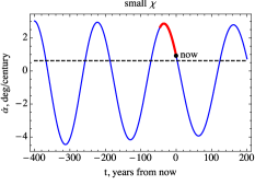
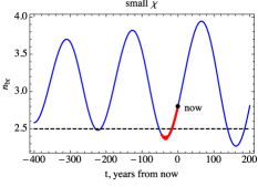
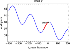
Figure 7: Similar to Fig. 6, but for the small $\chi$ case. The parameters of this solution at $t=0$ are: $\alpha=60^{\circ}$, $\theta=59.1^{\circ}$, $\chi=1^{\circ}$. The solution shows order of magnitude agreement with observations. Note that for $\chi\ll 1$, i.e., when the magnetic and stellar symmetry axes are close to each other, $\alpha$ shows a secularly decreasing trend, as opposed to the large $\chi$ case, shown in Fig. 6, where $\alpha$ oscillates about a constant value.

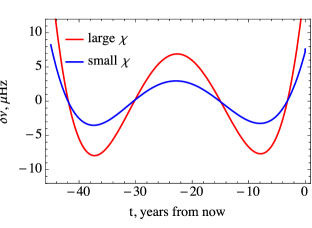
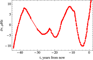
Figure 8: Comparison of our model results and the observed frequency residual for Crab pulsar. [Left panel:] The frequency residuals vs time in our numerical simulations are shown with the red line for the case of large $\chi$ and the blue line for the case of small $\chi$. [Right panel:] The observed frequency residual vs time. Despite a large number of glitches in the data, our model shows an order of magnitude agreement with the observations. Note that the variations in the frequency residual occur not on the precession period but on a much larger time scale set by the fourth-order frequency derivative. In order to observe variations caused by precession (as in the case of PSR B1828-11), one needs to observe Crab pulsar for at least several precession periods.

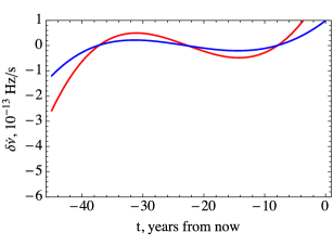
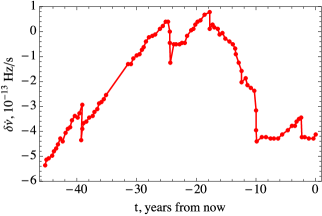
Figure 9: The comparison of our Crab modelling results to the observations of the frequency derivative residual. [Left panel] The red line shows the simulated residuals for the large $\chi$ case and the blue line for the small $\chi$ case. [Right panel] Observed timing residuals. As in Fig. 8, our modelling results show an order of magnitude agreement with the observed values, as expected given the large number of Crab’s glitches that are not included into our modelling.

For isolated pulsars it is common to consider a dimensionless quantity called the braking index:

$$n_{\rm br} \equiv\frac{\ddot{\Omega}\Omega}{\dot{\Omega}^{2}}.$$ (58)

A spherical pulsar rotating in vacuum has

$$n_{\rm br}^{\rm VAC} =3+2\tan^{-2}\alpha\geq 3,$$ (59)

and a spherical MHD pulsar has

$$n_{\rm br}^{\rm MHD} =3+2\frac{\sin^{2}\alpha\cos^{2}\alpha}{(1+\sin^{2}\alpha)^{2}},~{}~{}3\leq n_{\rm br}^{\rm MHD}\leq 3.25.$$ (60)

Although $n_{\rm br}\geq 3$ for both models, observations show values not only less than 3 (e.g., the Crab pulsar has $n_{\rm br}\approx 2.5$) but even negative values. In fact, braking indices span the range from $-10^{6}$ to $+10^{6}$. If the pulsar experiences precession, it can have an arbitrary value of braking index both larger and smaller than 3, and can also be negative. As we show in Figures 6 and 7, the observed braking index of the Crab pulsar can be easily reproduced by our model.

We note that our precessing solutions show that the near-linear increase of the inclination angle of Crab pulsar will be inevitably followed by its decrease, and the minimal timescale for this switch is $\sim 100$ years. It is possible that deviations from the linear increase could be detectable on much shorter timescales, perhaps as short as $\sim 20$ years.

For the Crab pulsar, it is quite difficult to fit the timing residuals data due to the presence of glitches that are not included into our modelling. Nevertheless, we can compare the characteristic amplitudes of simulated to observed timing residuals, as shown in Figs. 8 and 9. In both small and large $\chi$ cases, our modelling results and observations agree to within an order of magnitude.

We conclude that precession is a plausible explanation of observed behaviour of Crab pulsar, quantitatively reproducing the range of observed frequency derivatives, the braking index, inclination angle derivative, and the timing residuals.

6 Discussion

In this Section, we discuss and compare our results for the Crab pulsar and pulsar B1828-11, and discuss astrophysical implications.

6.1 Vacuum vs. Plasma-filled Magnetospheres

We start by discussing the differences between the vacuum and MHD models in terms of their effect on the timing residuals. As we showed in Sec. 5.3, the anomalous torque has no effect on the timing residuals. This means that the uncertainties in its estimate do not affect our results. From the point of view of timing residuals, the difference between vacuum and MHD models is evident in the denominator of equation (51):

$$f^{\rm MHD}=\frac{\sin 2\theta_{0}\sin 2\chi}{4-A(\theta_{0},\chi)},$$ (61)

which for the vacuum case takes the following form:

$$f^{\rm VAC}=\frac{\sin 2\theta_{0}\sin 2\chi}{2-A(\theta_{0},\chi)},$$ (62)

where $A(\theta,\chi)=2\cos^{2}\theta\cos^{2}\chi+\sin^{2}\theta\sin^{2}\chi$. Since the observed timing residuals, given by eq. (50), are observationally inferred to be very small, i.e., $\delta\dot{P}/\dot{P}\ll 1$, the $f$ factors given by eqs. (61) and (62) are also $\ll 1$. To get a good fit, the values of $\theta$ and $\chi$ must be either near zero $0$ or $90$ degrees. Importantly, the two-peak structure, such as seen in the residuals of the pulsar B1828-11, is reproduced only for $g=\tan\chi\tan\theta_{0}/4\sim 1$ (see eq. 52). So, either $\theta$ is close to 0 and $\chi$ is close to 90 degrees or vice versa. Thus, the angular dependence in the denominators of equations (61) and (62) is negligible, i.e., $A\ll 1$, and

$$f^{\rm MHD}=0.5f^{\rm VAC}.$$ (63)

The twice as small residuals implied by plasma-filled models lead to a larger space of allowed solutions (Sec. 5.3) and allow values of $\chi$ or $\theta$ to be further away from the extreme values (e.g., $0$ or $90$ degrees) than in the vacuum models. For instance, previous studies of pulsar B1828-11 in the context of the vacuum model (Jones & Andersson, 2001; Link & Epstein, 2001) found $\theta\lesssim 1$ degree while our plasma-filled model gives $\theta=5$ degrees.

The effect of stellar non-sphericity on the long-term evolution of pulsar parameters depends on the magnitude of the $\chi$ angle between the magnetic moment and the principle axis of the star. In the case of large $\chi$, the angles $\theta$ and $\alpha$ oscillate at the precession period and their averages show no long-term trends, as seen in Fig. 6.

In the case of small $\chi$, the values of $\alpha$ and $\chi$ also oscillate on the precession timescale but undergo a secular decrease over longer timescales, as seen in the right panel of Fig. 3: both vacuum and MHD pulsars evolve toward alignment. Thus, if most pulsars are in the small $\chi$ case, non-sphericity effects will have very few implications for the pulsar statistics, which favors an alignment trends on the timescale of $10^{6}{-}10^{7}$ years in agreement with spherical pulsar models (Tauris & Manchester 1998; Young et al. 2010; Gullón et al. 2014). The vacuum pulsars approach the alignment exponentially fast and the MHD pulsars do so much more slowly, as a power-law in time. These long-term evolutionary trends are quantitatively similar to those for spherically-symmetric pulsars (Philippov et al., 2014). However, unlike the spherical pulsars, which evolve toward complete alignment ($\alpha=0$), non-sphericity causes the inclination angle to stabilise at a finite value, $\alpha_{\rm stab}>0$. The precise value of $\alpha_{\rm stab}$ can differ between vacuum and MHD models: for instance, for the parameters chosen in Fig. 3, an MHD pulsar stabilises at $\alpha^{\rm MHD}_{\rm stab}=3.46$ deg and a vacuum pulsar at a much smaller value, $\alpha^{\rm VAC}_{\rm stab}=0.35$ deg. Note that since vacuum pulsars align exponentially fast, they can reach stabilization after $10^{5}$ years, which is much shorter than the pulsar lifetime. In contrast, stabilisation can take $\sim 10^{8}$ years for MHD pulsars, and it is unclear how many MHD pulsars reach stabilisation in their lifetime.

6.2 Crab pulsar vs. B1828-11

We demonstrated that the increase in time of Crab pulsar’s inclination angle could be easily explained if this pulsar experiences precession, confirming our earlier expectations (Philippov et al., 2014). A precession period, $T_{\rm prec}\sim 100$ years, and rotational period, $P=0.033$ s, imply a rather small stellar ellipticity $\varepsilon_{\rm Crab}\lesssim 10^{-11}$ (see Tab. 3). Indeed, this value is much smaller than the minimum allowed value of ellipticity for the pulsar B1828-11, $\varepsilon_{1828}\sim 10^{-8}$.

When this work was completed, a preprint by Zanazzi & Lai (2015) was posted on the archives. They considered a precession model for the Crab pulsar in the framework of vacuum magnetosphere and obtained $\varepsilon=4\times 10^{-11}$, slightly higher than our value. Their geometrical parameters are more extreme, as one would expect from a vacuum model: $\chi=0.15$ deg (vs $\ll 1$ deg in MHD models) in the small $\chi$ case and $\theta=0.1$ deg ($\ll 2$ deg) in the large $\chi$ case.

For the Crab pulsar, the MHD spindown formula (11) implies a surface magnetic field $B_{12}=2.33$ for a characteristic pulsar obliquity angle $\alpha=60$ deg (the magnetodipole formula gives a slightly larger value $B_{12}=3.78$). The estimate (33) for magnetically-induced ellipticity gives $\varepsilon=0.6\times 10^{-11}$, i.e., very close to the inferred value, so Crab’s ellipticity could be accounted for by a magnetically-induced deformation of its crust. We note that the we can only place a rough lower limit on the precession period of the Crab pulsar, and it could be significantly longer than $100$ years. Long-term observations in the next several decades might help to break this degeneracy and measure the precession period if it is not much longer than a century.

The pulsar B1828-11 has approximately the same surface magnetic field, but its inferred ellipticity is $3$ orders of magnitude larger, $\epsilon\simeq 10^{-8}$. One way to reconcile this difference from the Crab pulsar is to postulate strong ($\sim 10^{14}$ G) internal magnetic fields in the pulsar B1828-11. Another possible explanation for the difference in the values of ellipticities can be found in the framework of rotational ellipticity model. Equation (31) gives very large ellipticity values. However, as Jones & Andersson (2001) pointed out, only a small fraction of this deformation participates in the precession due to the pinning of magnetic vortexes to the crustal lattice. Crab is younger, has a lot of glitches, so, the pinning fraction is large and the effective ellipticity small. Since PSR B1828-11 is older, it is conceivable that it has a smaller pinning fraction and a larger effective ellipticity. In this context, it is interesting that all known pulsars that experience timing noise on the timescale of several years, have ages larger than that of B1828-11 (Lyne et al., 2010). Thus, we may expect that the older the pulsar, the larger the effective ellipticity that participates in precession. Dissipative processes in the stellar interior such as crust-core coupling may also affect the long-term evolution of the neutron star (Barsukov et al., 2014).

Pulsar B1828-11 does not show an observed interpulse, and this might seem at odds with our precessing solution, in which $\alpha$ is very close to 90 degrees. However, due to the uncertainties in the radio emission mechanism and the plasma distribution near the polar cap of nearly orthogonal rotators, it is not clear that an interpulse will necessarily be visible. It is possible that magnetospheric synchrotron absorption (Beskin & Philippov, 2012) can significantly damp the interpulse emission. More detailed investigation is needed to produce reliable models of the observed radio profiles of this pulsar and independently confirm the geometry inferred from precession models.

7 Conclusions

In this work, we presented the analysis of pulsar evolution that self-consistently takes into account magnetospheric plasma effects, as measured in 3D MHD simulations of pulsar magnetospheres. We showed that the MHD effects expand the allowed parameter space of pulsar precession solutions and thereby allow for less extreme solutions than the vacuum models. To facilitate the interpretation of pulsar timing residual curves, we developed an analytic model that converts the observed residuals into the pulsar geometrical parameters.

We applied this model to the timing residuals of PSR B1828-11 and obtained its parameters: e.g., stellar ellipticity and the orientation of the stellar ellipsoid, magnetic and rotational axes. With the best-fit parameters, both the period and period derivative timing residual curves are well-reproduced by our model. Our best-fitting values for the pulsar parameters are less extreme than in the vacuum models.

In the context of spherically-symmetric stars, it is expected that the magnetic and rotational axes of the pulsars evolve toward each other as the pulsar ages. Recently a puzzling observation of an opposite trend was reported for the Crab pulsar (Lyne et al., 2013). In this work, we showed that this surprising trend can be explained by the precession of a neutron star, in agreement with our earlier expectations (Philippov et al. 2014; see Zanazzi & Lai 2015 for a consideration of this effect in the vacuum approximation). The data is consistent with a precession period of the Crab pulsar that is as short as $\lesssim 100$ years. If the true precession period is not exceedingly larger than that, it could be measured in the next decades, warranting a continuous monitoring of the Crab pulsar.

Appendix A Analytical solution

In this section we describe analytical solution for pulsar precession. The exact solution could be treated as small perturbations of free precession motion. We describe free precession in Section A.1, perturbation caused by anomalous torque are discussed in Section A.2, effects of regular alignment torque are considered in Section A.3, two-peak structure in residuals are obtained in Section A.4 and we finally discuss the effects of the second ellipticity in Section A.5.

A.1 Free precession

For freely precessing body Euler’s equations of motion take the following form:

$$\dot{\boldsymbol{L}}+{\boldsymbol{\Omega}}\times\boldsymbol{L}=0.$$ (64)

These equations can be solved analytically (Landau & Lifshitz (1976)) in terms of Jacobian elliptic functions:

$$L_{1}/I\Omega_{0} = \sin\theta_{0}\times{\rm cn}(\omega_{\rm p}t,k\tan^{2}\theta_{0}),$$ (65)

$$L_{2}/I\Omega_{0} = \sin\theta_{0}\sqrt{1+k}\times{\rm sn}(\omega_{\rm p}t,k\tan^{2}\theta_{0}),$$ (66)

$$L_{3}/I\Omega_{0} = \cos\theta_{0}\times{\rm dn}(\omega_{\rm p}t,k\tan^{2}\theta_{0}),$$ (67)

where $k=I_{3}(I_{2}-I_{1})/I_{1}(I_{3}-I_{2})=\varepsilon_{12}(1+\varepsilon_{13})/(\varepsilon_{13}-\varepsilon_{12})\approx\varepsilon_{12}/(\varepsilon_{13}-\varepsilon_{12})$ and $\omega_{\rm p}=\varepsilon_{13}L\cos\theta_{0}/I_{3}\sqrt{1+k}\approx\varepsilon_{13}\Omega_{0}\cos\theta/\sqrt{1+k}$. The precession period is equal

$$\tau_{\rm prec}=\frac{P}{\varepsilon_{13}\cos\theta_{0}}\frac{2F(\pi/2,k\tan^{2}\theta_{0})}{\pi},$$ (68)

where $F(\phi,m)$ is the Legendre elliptic integral of the first kind.

In the case of $\varepsilon_{12}=0$, that is of an axisymmetric star, the solution takes on a much simpler form:

$$L_{1}/I\Omega_{0} = \sin\theta_{0}\times\cos(\omega_{\rm p}t),$$ (69)

$$L_{2}/I\Omega_{0} = \sin\theta_{0}\times\sin(\omega_{\rm p}t),$$ (70)

$$L_{3}/I\Omega_{0} = \cos\theta_{0},$$ (71)

where $\omega_{\rm p}=\varepsilon_{13}\Omega_{0}\cos\theta_{0}$ and $\Omega_{0}$ is the initial rotational frequency. In this case, the precession period is simply

$$\tau_{\rm prec}=P/\varepsilon_{13}\cos\theta_{0}.\quad{\rm(axisymmetric\ star)}$$ (72)

A.2 Effects of the anomalous torque

In reality the precession of radio pulsar is not free. In order to correctly describe it one have to solve the following equation:

$$\dot{\boldsymbol{L}} +{\boldsymbol{\Omega}}\times\boldsymbol{L}={\boldsymbol{K}}=$$ (73)

$$= K_{\rm aligned}\left(-2\frac{\boldsymbol{\Omega}}{\Omega}+\cos\alpha\frac{\boldsymbol{\mu}}{\mu}+\frac{k_{3}\sin\alpha\cos\alpha}{\Omega R/c}\frac{\boldsymbol{\Omega}\times\boldsymbol{\mu}}{|\Omega\times\mu|}\right),$$

where we already use MHD torques with $k_{0}=k_{1}=k_{2}=1$.

After we normalize this equation by $I\Omega_{0}$ and set ${\boldsymbol{L}}=I(\boldsymbol{\Omega}+\varepsilon_{12}\Omega_{2}\boldsymbol{e}_{2}+\varepsilon_{12}\Omega_{3}\boldsymbol{e}_{3})$, we obtain the following expression:

$$\dot{\boldsymbol{\omega}} +\frac{1}{\tau_{\rm prec}}\left[\frac{\dot{\omega}_{3}}{\Omega_{0}}\boldsymbol{e}_{3}+\frac{\varepsilon_{12}}{\varepsilon_{13}}\frac{\dot{\omega}_{2}}{\Omega_{0}}\boldsymbol{e}_{2}+\omega_{3}\boldsymbol{\omega}\times\boldsymbol{e}_{3}+\frac{\varepsilon_{12}}{\varepsilon_{13}}\omega_{3}\boldsymbol{\omega}\times\boldsymbol{e}_{2}\right]=$$ (74)

$$= \frac{\omega^{3}}{\tau}\left[-2\frac{\boldsymbol{\omega}}{\omega}+\cos\alpha\frac{\boldsymbol{\mu}}{\mu}\right]+\frac{\omega^{2}}{\tau_{\rm anom}}\sin\alpha\cos\alpha\frac{\boldsymbol{\omega}\times\boldsymbol{\mu}}{|\omega\times\mu|},$$

where $\omega_{i}=\Omega_{i}/\Omega_{0}$, $\tau_{\rm prec}=1/\varepsilon_{13}\Omega_{0}$, $\tau=I\Omega_{0}/K_{\rm aligned}^{0}$ and $\tau_{\rm anom}=(\Omega_{0}R/c)I\Omega_{0}/k_{3}K_{\rm aligned}^{0}$.

In this section we consider $\varepsilon_{12}=0$ and $\tau_{\rm prec}\ll\tau_{\rm anom}\ll\tau$. This approximation is well-satisfied for pulsars and we can treat torque effects as perturbations of free precession motion.

Using these assumptions and the relation $\cos\alpha=\omega_{1}\sin\chi+\omega_{3}\cos\chi$ we can write the equations for perturbations $\delta\omega_{i}$ in the following way:

$$\delta\dot{\omega}_{1} +\frac{\omega_{3}\delta\omega_{1}+\omega_{1}\delta\omega_{3}}{\tau_{\rm prec}}=$$

$$=\frac{\omega^{2}}{\tau_{\rm anom}}(\omega_{1}\sin\chi+\omega_{3}\cos\chi)\omega_{2}\cos\chi,$$ (75)

$$\delta\dot{\omega}_{2} -\frac{\omega_{3}\delta\omega_{2}+\omega_{2}\delta\omega_{3}}{\tau_{\rm prec}}=$$

$$=\frac{\omega^{2}}{\tau_{\rm anom}}(\omega_{1}\sin\chi+\omega_{3}\cos\chi)(\omega_{3}\sin\chi-\omega_{1}\cos\chi),$$ (76)

$$\delta\dot{\omega}_{3} =-\frac{\omega^{2}}{\tau_{\rm anom}}(\omega_{1}\sin\chi+\omega_{3}\cos\chi)\omega_{2}\sin\chi.$$ (77)

Here we neglect the effects of $\tau$ and the first two terms in brackets in LHS of equation (74) as they are much smaller than $\dot{\omega}$.

Now we set $\omega_{i}$ to be equal to their unperturbed values and solve the system of linear differential equations (A.2)-(77). This is the system of linear differential equations with constant coefficients, so it is straightforward to find a solution:

$$\delta\omega_{1}= -\psi_{0}+\psi_{1}\omega_{\rm p}t\sin\omega_{\rm p}t-\psi_{2}\cos\omega_{\rm p}t-$$

$$-\psi_{3}\sin^{2}\omega_{\rm p}t\cos\omega_{\rm p}t,$$ (78)

$$\delta\omega_{2}= -\psi_{1}\omega_{\rm p}t\cos\omega_{\rm p}t+\psi_{3}\sin\omega_{\rm p}t\cos^{2}\omega_{\rm p}t$$ (79)

$$\delta\omega_{3}= \psi_{0}\tan\theta_{0}\cos\omega_{\rm p}t+\psi_{2}\tan\theta_{0}\cos^{2}\omega_{\rm p}t,$$ (80)

where $\omega_{\rm p}=\cos\theta_{0}/\tau_{\rm prec}$ and

$$\psi_{0} =\frac{\tau_{\rm prec}}{\tau_{\rm anom}}\sin\chi\cos\chi\cos\theta_{0},$$ (81)

$$\psi_{1} =\frac{\tau_{\rm prec}}{\tau_{\rm anom}}\left(\cos^{2}\chi\sin\theta_{0}-\sin^{2}\chi\frac{2\sin\theta_{0}-\sin^{3}\theta_{0}}{4\cos^{2}\theta_{0}}\right),$$ (82)

$$\psi_{2} =\frac{\tau_{\rm prec}}{\tau_{\rm anom}}\sin^{2}\chi\sin\theta_{0}/2,$$ (83)

$$\psi_{3} =\frac{\tau_{\rm prec}}{\tau_{\rm anom}}\frac{\sin^{2}\chi}{4}\frac{\sin^{3}\theta_{0}}{\cos^{2}\theta_{0}}.$$ (84)

It is important to notice that the amplitude of $\omega$ remains unperturbed: $\omega_{1}\delta\omega_{1}+\omega_{2}\delta\omega_{2}+\omega_{3}\delta\omega_{3}\equiv 0$. This is because the anomalous torque is perpendicular to $\boldsymbol{\Omega}$ and thus cannot change its amplitude.

On the other hand, anomalous torque causes the changes in $\theta$ since $\delta\omega_{3}=-\sin\theta_{0}\delta\theta$.

$$\delta\theta=-\frac{\cos\omega_{\rm p}t}{\cos\theta_{0}}(\psi_{0}+\psi_{2}\cos\omega_{\rm p}t).$$ (85)

The maximum deviation is given by

$$\max|\theta-\theta_{0}|\approx\frac{\tau_{\rm prec}}{\tau_{\rm anom}}\frac{\sin 2\chi+\sin^{2}\chi\tan\theta_{0}}{2}.$$ (86)

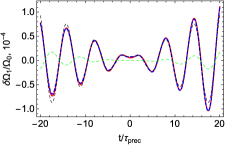
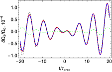
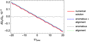
Figure 10: The comparison of exact numerical solution with analytical asymptotic for $\chi=88.5$ deg, $\theta_{0}=6$ deg. The figure shows an excellent agreement of numerical solution and observations. This allows us to use simple analytical expressions (56)–(57) instead of numerical procedures.

A.3 Effects of the alignment torque

If one considers in equation (74) the contribution of alignment torque, it is possible to complete exactly the same procedure as in Section A.2. The solution in this case is quite different:

$$\delta\omega_{1} =\phi_{2}\sin 2\omega_{\rm p}t-\phi_{3}\omega_{\rm p}t\cos\omega_{\rm p}t+\phi_{4}\omega_{\rm p}^{2}t^{2}\sin\omega_{\rm p}t,$$ (87)

$$\delta\omega_{2} =\phi_{0}+\phi_{1}\cos\omega_{\rm p}t-\phi_{2}\cos 2\omega_{\rm p}t-\phi_{3}\omega_{\rm p}t\sin\omega_{\rm p}t-$$

$$-\phi_{4}\omega_{\rm p}^{2}t^{2}\cos\omega_{\rm p}t,$$ (88)

$$\delta\omega_{3} =(\phi_{2}\sin\omega_{\rm p}t-\phi_{4}\omega_{\rm p}t)\cot\theta_{0},$$ (89)

where

$$\phi_{0} =\frac{\tau_{\rm prec}}{\tau}\frac{2-\tan^{2}\theta_{0}}{2}\sin\chi\cos\chi,$$ (90)

$$\phi_{1} =\frac{\tau_{\rm prec}}{\tau}\frac{\sin^{2}\chi\tan\theta_{0}}{2},$$ (91)

$$\phi_{2} =\frac{\tau_{\rm prec}}{\tau}\sin\chi\cos\chi\tan^{2}\theta_{0},$$ (92)

$$\phi_{3} =\frac{\tau_{\rm prec}}{\tau}\frac{7+\cos 2\chi}{4}\tan\theta_{0},$$ (93)

$$\phi_{4} =\frac{\tau_{\rm prec}}{\tau}\frac{3-\cos 2\chi}{4}\tan\theta_{0}.$$ (94)

If we combine the effects of both alignment and anomalous torque we obtain the total perturbation. Fig. 10 compares exact numerical solution with total perturbation as well as the perturbations caused by alignment and anomalous torques separately.

The alignment torque causes $\omega$ to change. The perturbation to the frequency takes the following form:

$$\delta\omega =\omega_{1}\delta\omega_{1}+\omega_{2}\delta\omega_{2}+\delta\omega_{3}\omega_{3}=$$ (95)

$$=-\frac{\tau_{\rm prec}}{\tau}\omega_{\rm p}t(3-\cos 2\chi+7\tan^{2}\theta_{0}-\cos 2\chi\tan^{2}\theta_{0})\cos\theta_{0}/2+$$

$$+\frac{\tau_{\rm prec}}{\tau}\sin 2\chi\sin\theta_{0}(\sin\omega_{\rm p}t+1/8\tan\theta_{0}\tan\chi\sin 2\omega_{\rm p}t).$$

Here we can see spin down as well as the two harmonics that are actually presented in observations.

Summing up, the observed residual curves are the first-order perturbation over free precession motion caused by the alignment torque. The first-order residual has up to two harmonics.

A.4 Two-peak structure

The frequency residual $\delta\omega$ could be found in much more simple way. In order to find it we multiply equation (74) by $\boldsymbol{\omega}$:

$$\dot{\omega}=-\frac{\omega_{3}\dot{\omega}_{3}+\varepsilon_{12}/\varepsilon_{13}\omega_{2}\dot{\omega}_{2}}{\omega\tau_{\rm prec}\Omega_{0}}-\frac{\omega^{3}(1+\sin^{2}\alpha)}{\tau}$$ (96)

Puting zero-order solution for $\varepsilon_{12}=0$ in RHS of this equation gives the following equation:

$$\dot{\omega} =-\frac{1}{\tau}(2-\cos^{2}\theta_{0}\cos^{2}\chi-1/2\sin^{2}\theta_{0}\sin^{2}\chi)+$$ (97)

$$+\frac{1}{\tau}\frac{\sin 2\theta_{0}\sin 2\chi}{2}(\cos\omega_{\rm p}t+\cos 2\omega_{\rm p}t\tan\theta_{0}\tan\chi/4).$$ (98)

The first term of this expression is the observed spindown. Having that we can rewrite this equation in the following way:

$$\dot{\omega}=-\frac{\dot{P}^{\rm obs}}{P^{\rm obs}}\left(1-\frac{\sin 2\theta_{0}\sin 2\chi(\cos\omega_{\rm p}t+\cos 2\omega_{\rm p}t\tan\theta_{0}\tan\chi/4)}{4-2\cos^{2}\theta_{0}\cos^{2}\chi-\sin^{2}\theta_{0}\sin^{2}\chi}\right).$$ (99)

Finally, the residual in $\dot{P}$ now takes a form

$$\delta\dot{P}=-\dot{P}^{\rm obs}f(\theta_{0},\chi)(\cos\omega_{\rm p}t+g(\theta_{0},\chi)\cos 2\omega_{\rm p}t)$$ (100)

with

$$f(\theta_{0},\chi)=\frac{\sin 2\theta_{0}\sin 2\chi}{4-2\cos^{2}\theta_{0}\cos^{2}\chi-\sin^{2}\theta_{0}\sin^{2}\chi},$$ (101)

$$g(\theta,\chi)=\tan\theta_{0}\tan\chi/4.$$ (102)

The amplitude of residual is proportional to $\sin 2\theta_{0}\sin 2\chi$. If we have residuals which are much smaller than $\dot{P}^{\rm obs}$ (which is usually the case), $\theta_{0}$ and $\chi$ should be close either to 0 or to 90 deg. As observed residuals are much smaller than $\dot{P}^{\rm obs}$ and we observe two-bump structure (so, $g(\theta_{0},\chi)\approx 1$), one of the angles should be very close to 0, and another one – to 90 deg.

A.5 Effects of the second ellipticity

For $\varepsilon_{12},\varepsilon_{23}\ll 1$, one can show that

$$\frac{\varepsilon_{12}}{\varepsilon_{13}}\approx\frac{k}{k+1}.$$ (103)

In this case, zero-order solution implies

$$\omega_{3}\dot{\omega}_{3}+\varepsilon_{12}/\varepsilon_{23}\omega_{2}\dot{\omega}_{2}\equiv 0.$$ (104)

The solution for perturbations takes now very similar form:

$$\delta\dot{P}=-\dot{P}^{\rm obs}f(\theta_{0},\chi)\mathcal{P}(\theta_{0},\chi,t)$$ (105)

with

$$\mathcal{P} ={\rm cn}(\omega_{p}t){\rm dn}(\omega_{p}t)+{\rm cn}(2\omega_{p}t)\frac{2g(\theta_{0},\chi)}{(1+{\rm dn}(2\omega_{p}t))}+$$ (106)

$$+({\rm dn}(2\omega_{p}t)-1)\left(\frac{g(\theta_{0},\chi)}{(1+{\rm dn}(2\omega_{p}t))}+\frac{g(\theta_{0},\chi)^{-1}}{8(1+{\rm cn}(2\omega_{p}t))}\right).$$

It shows that the second ellipticity does not qualitatively change the behaviour of solution and only influences the precession period (see eq. (68)).

References

- Barsukov et al. (2014) Barsukov D. P., Goglichidze O. A., Tsygan A. I., 2014, MNRAS, 444, 1318
- Belyaev (2015) Belyaev M. A., 2015, New Ast., 36, 37
- Beskin et al. (1993) Beskin V. S., Gurevich A. V., Istomin Y. N., 1993, Physics of the pulsar magnetosphere. Cambridge University Press
- Beskin & Philippov (2012) Beskin V. S., Philippov A. A., 2012, MNRAS, 425, 814
- Cerutti et al. (2015) Cerutti B., Philippov A., Parfrey K., Spitkovsky A., 2015, MNRAS, 448, 606
- Chen & Beloborodov (2014) Chen A. Y., Beloborodov A. M., 2014, ApJ, 795, L22
- Contopoulos et al. (1999) Contopoulos I., Kazanas D., Fendt C., 1999, ApJ, 511, 351
- Deutsch (1955) Deutsch A. J., 1955, Annales d’Astrophysique, 18, 1
- Glendenning (1997) Glendenning N. K., 1997, Journal of Physics G Nuclear Physics, 23, 2013
- Goldreich (1970) Goldreich P., 1970, ApJ, 160, L11
- Goldreich & Julian (1969) Goldreich P., Julian W. H., 1969, ApJ, 157, 869
- Gullón et al. (2014) Gullón M., Miralles J. A., Viganò D., Pons J. A., 2014, MNRAS, 443, 1891
- Horowitz & Kadau (2009) Horowitz C. J., Kadau K., 2009, Physical Review Letters, 102, 191102
- Igoshev & Popov (2013) Igoshev A. P., Popov S. B., 2013, MNRAS, 432, 967
- Jones & Andersson (2001) Jones D. I., Andersson N., 2001, MNRAS, 324, 811
- Kalapotharakos & Contopoulos (2009) Kalapotharakos C., Contopoulos I., 2009, A&A, 496, 495
- Landau & Lifshitz (1976) Landau L. D., Lifshitz E. M., 1976, Electrodynamics of continuous media. Pergamon Press
- Link & Epstein (2001) Link B., Epstein R. I., 2001, ApJ, 556, 392
- Lyne et al. (2013) Lyne A., Graham-Smith F., Weltevrede P., Jordan C., Stappers B., Bassa C., Kramer M., 2013, Science, 342, 598
- Lyne et al. (2010) Lyne A., Hobbs G., Kramer M., Stairs I., Stappers B., 2010, Science, 329, 408
- Lyne et al. (2015) Lyne A. G., Jordan C. A., Graham-Smith F., Espinoza C. M., Stappers B. W., Weltevrede P., 2015, MNRAS, 446, 857
- Melatos (2000) Melatos A., 2000, MNRAS, 313, 217
- Michel & Goldwire (1970) Michel F. C., Goldwire Jr. H. C., 1970, Astrophys. Lett., 5, 21
- Munk & MacDonald (1975) Munk W. H., MacDonald G. J. F., 1975, The rotation of the earth: a geophysical discussion.. Cambridge University Press
- Philippov et al. (2014) Philippov A., Tchekhovskoy A., Li J. G., 2014, MNRAS, 441, 1879
- Philippov & Spitkovsky (2014) Philippov A. A., Spitkovsky A., 2014, ApJ, 785, L33
- Philippov et al. (2015) Philippov A. A., Spitkovsky A., Cerutti B., 2015, ApJ, 801, L19
- Popov & Turolla (2012) Popov S. B., Turolla R., 2012, Ap&SS, 341, 457
- Spitkovsky (2006) Spitkovsky A., 2006, ApJ, 648, L51
- Stairs et al. (2000) Stairs I. H., Lyne A. G., Shemar S. L., 2000, Nature, 406, 484
- Tauris & Manchester (1998) Tauris T. M., Manchester R. N., 1998, MNRAS, 298, 625
- Tchekhovskoy et al. (2015) Tchekhovskoy A., Philippov A., Spitkovsky A., 2015, ArXiv e-prints
- Tchekhovskoy et al. (2013) Tchekhovskoy A., Spitkovsky A., Li J. G., 2013, MNRAS, 435, L1
- Young et al. (2010) Young M. D. T., Chan L. S., Burman R. R., Blair D. G., 2010, MNRAS, 402, 1317
- Zanazzi & Lai (2015) Zanazzi J. J., Lai D., 2015, ArXiv:1503.01486