Minimal subspace rotation on the Stiefel manifold for stabilization and enhancement of projection-based reduced order models for the compressible Navier-Stokes equations

Abstract

For a projection-based reduced order model (ROM) of a fluid flow to be stable and accurate, the dynamics of the truncated subspace must be taken into account. This paper proposes an approach for stabilizing and enhancing projection-based fluid ROMs in which truncated modes are accounted for a priori via a minimal rotation of the projection subspace. Attention is focused on the full non-linear compressible Navier-Stokes equations in specific volume form as a step toward a more general formulation for problems with generic non-linearities. Unlike traditional approaches, no empirical turbulence modeling terms are required, and consistency between the ROM and the full order model from which the ROM is derived is maintained. Mathematically, the approach is formulated as a trace minimization problem on the Stiefel manifold. The reproductive as well as predictive capabilities of the method are evaluated on several compressible flow problems, including a problem involving laminar flow over an airfoil with a high angle of attack, and a channel-driven cavity flow problem.

1 Introduction

The past several decades have seen an exponential growth of computer processing speed and memory capacity. The massive, complex simulations that run on supercomputers allow exploration of fields for which physical experiments are too impractical, hazardous, and/or costly. A striking number of these fields require computational fluid dynamics (CFD) models and simulations. Accurate and efficient CFD simulations are critical to many defense, climate and energy missions, e.g., simulations aimed to design and qualify nuclear weapons components carried within an aircraft weapons bay; global climate simulations aimed to predict anticipated twenty-first century sea-level rise; aero-elastic simulations for optimal design of wind systems for power generation.

Unfortunately, even with the aid of massively parallel next-generation computers, CFD simulations for applications such as these are still too expensive for real-time and multi-query applications such as uncertainty quantification (UQ), optimization and control design. Reduced order modeling is a promising tool for bridging the gap between high-fidelity, and real-time simulations/UQ. Reduced order models (ROMs) are derived from a sequence of high-fidelity simulations but have a much lower computational cost. Hence, ROMs can enable real-time simulations of complex systems for more rapid analysis, control and decision-making in the presence of uncertainty.

Most existing ROM approaches are based on projection. In projection-based reduced order modeling, the state variables are approximated in a low-dimensional subspace. There exist a number of approaches for calculating this low-dimensional subspace, e.g., Proper Orthogonal Decomposition (POD) [44, 19], Dynamic Mode Decomposition (DMD) [38, 41] balanced POD (BPOD) [35, 49], balanced truncation [17, 27], and the reduced basis method [39, 47]. In all of these methods, a basis for the low-dimensional subspace is obtained from a basis for a higher-dimensional subspace through truncation – the removal of modes that are believed to be unimportant in representing a problem solution. Typically, the size of the reduced basis is chosen according to an energy criterion: modes with low energy are discarded, so that the reduced basis subspace is spanned by the highest energy modes. Although truncated modes are negligible from a data compression point of view, they are often crucial for representing solutions to the dynamical flow equations. Dynamics of the truncated orthogonal subspace must be taken into account for to ensure stability and accuracy of the ROM.

For linear systems, a variety of techniques for generating low-dimensional projection- based ROMs with rigorous stability guarantees and accuracy bounds are available [17, 27, 1, 23]. Equivalent results are lacking for nonlinear systems. Traditionally, low-dimensional ROMs of fluid flows have been stabilized and enhanced using empirical turbulence models. In this approach, the nonlinear dynamics of the truncated subspace are modeled using additional constant and linear terms in the ROM system of ordinary differential equations (ODEs) [2, 34, 12, 14]. More recently, nonlinear eddy-viscosity models have also been proposed [30, 28, 20, 32]. One downside of turbulence models is that they destroy consistency between the Navier-Stokes partial differential equations (PDEs) and the ODE system of the ROM. Accurately identifying and matching free coefficients of the turbulence models is another challenge. Moreover, these methods are usually limited to the incompressible Navier-Stokes equations.

Consider, for concreteness, the POD/Galerkin approach to model reduction applied to the incompressible Navier-Stokes equations. For these equations, the natural choice of inner product for the Galerkin projection step of the model reduction procedure is the $L^{2}$ inner product. This is because, in these models, the solution vector is taken to be the velocity vector $\mathbf{u}$, so that $||\mathbf{u}||_{2}$ is a measure of the global kinetic energy in the domain, and the POD modes optimally represent the kinetic energy present in the ensemble from which they were generated. The same is not true for the compressible Navier-Stokes equations. Hence, if a compressible fluid ROM is constructed in the $L^{2}$ inner product (a common choice of inner product in projection-based model reduction), the ROM solution may not satisfy the conservation relation implied by the governing equations, and may exhibit non-physical instabilities [37].

Unfortunately, ROM instability is a real problem for many compressible flow problems: as demonstrated in [6, 9, 7, 22], a compressible fluid POD/Galerkin ROM might be stable for a given number of modes, but unstable for other choices of basis size. Several researchers have proposed ways to circumvent this difficulty through the careful construction of an energy-based inner product for the projection step of the model reduction. Rowley et al. [37] show that Galerkin projection preserves the stability of an equilibrium point at the origin if the ROM is constructed in an energy–based inner product. Barone et al. [7], Kalashnikova et al. [22] demonstrate that a symmetry transformation leads to a stable formulation for a Galerkin ROM for the linearized compressible Euler equations and nonlinear compressible Navier-Stokes equations with solid wall and far-field boundary conditions. Serre et al. [42] propose applying the stabilizing projection developed by Barone et al. [7], Kalashnikova et al. [22] to a skew-symmetric system constructed by augmenting a given linear system with its adjoint system. The downside to these methods is that they are inherently embedded methods: access to the governing PDEs and/or the code that discretizes these PDEs is required.

Other ROM approaches, e.g., the Gauss-Newton with Approximated Tensors (GNAT) method of Carlberg et al. [10], have better stability properties, as they formulate the ROM at the fully discrete level. The drawback of this approach is that an additional layer of approximation – usually called hyper-reduction — is required to gain computational speed-up. Moreover, the approach lacks stability guarantees for low-dimensional expansions.

In this paper, a stabilization and enhancement approach to ROMs for the compressible Navier-Stokes equations is developed. The approach is an extension of the methodology developed in [3, 5] specifically for the incompressible Navier-Stokes equations. The specific volume ($\zeta$–) form of the compressible Navier-Stokes equations is utilized. Since these equations have polynomial (quadratic) nonlinearities, the Galerkin projection can be computed offline, once and for all; no hyper-reduction is required [21]. Unlike traditional eddy-viscosity-based stabilization methods, the proposed approach requires no additional empirical turbulence modeling terms – truncated modes are accounted for a priori via a minimal rotation of projection subspace. The method is also non-intrusive, as it operates only on the matrices and tensors defining a ROM ODE system, which are stabilized through the offline solution of a small trace minimization problem on the Stiefel manifold. The proposed new approach can be interpreted as a combination of several previously developed ideas. Following Iollo et al. [21], we propose to stabilize and enhance projection-based ROMs by modifying the projection subspace in order to capture more of the low-energy, but high dissipative scales of the flow solution. Similarly to Amsallem and Farhat [1], a rotation of the projection subspace is used to achieve this goal. Specifically, a larger set of basis is linearly superimposed to provide a smaller set of basis that generate a stable and accurate ROM. Finally, in the spirit of most previously proposed eddy-viscosity-based turbulence models, the eigenvalues of the linear part of the Galerkin system of ODEs are used as a proxy to guide the stabilization algorithm.

The remainder of this paper is organized as follows. In § 2, the standard projection-based model reduction approach is outlined in the context of the specific volume form of the compressible Navier-Stokes equations. Also overviewed is the POD method for constructing an optimal reduced basis, and some eddy-viscosity based closure models used for accounting for modal truncation. The proposed methodology of “rotating” the projection subspace into a more dissipative regime to better resolve the small, energy dissipative scales of the flow is detailed in § 3. Here, the approach is formulated mathematically as a constrained optimization problem on the Stiefel manifold. In § 4, the performance of the proposed method is evaluated on several compressible flow problems, including a problem involving a laminar flow over an airfoil with a high angle of attack, and a channel-driven cavity flow problem. Finally, conclusions are offered in § 5.

2 Projection-based model reduction for nonlinear compressible flow

In this section the standard projection-based model reduction approach is laid out. In § 2.1 the approach for a general nonlinear system is presented while in § 2.2 the approach is applied to the compressible Navier-Stokes equations. The POD method for calculating a reduced basis using a set of snapshots from a high-fidelity simulation is outlined in § 2.3, followed by a brief overview of eddy-viscosity-based closure models that account for modes truncated in the application of the POD method (§  2.4).

2.1 Nonlinear projection-based model order reduction

Consider a dynamical system of the form:

$${\frac{d}{{dt}}\bm{w}}=\bm{F}\left(\bm{w}\right),$$ (1)

where $\bm{F}$ is the propagator in $H$, a Hilbert space. In fluid flows, the state variable $\bm{w}=\bm{w}(\bm{x},t)\in H$ depends on space $\bm{x}\in\Omega$, $\Omega$ being the flow domain, and time $t\in\left[{0,T}\right]$, $T$ representing the period of integration. Then, the propagator $\bm{F}$ contains spatial derivatives. The associated Hilbert space of square-integrable functions $L^{2}(\Omega)$ is equipped with the standard inner product for its elements $\bm{w}\in L^{2}(\Omega)$, defined by:

$$\left({\bm{w},\bm{w}}\right)_{\Omega}:=\int\limits_{\Omega}\bm{w}\cdot\bm{w}\>d\bm{x}.$$ (2)

In the Galerkin ROM approach, the governing variable, $\bm{w}(\bm{x},t)$ is discretized using basis functions (modes) $\left\{\bm{w}_{i}(\bm{x})\right\}_{i=1}^{n}\in H$ with corresponding mode coefficients $\left\{a_{i}(t)\right\}_{i=1}^{n}$

$$\bm{w}(\bm{x},t)\approx\bm{w}_{0}(\bm{x})+\bm{w}^{[1..n]}(\bm{w},t):=\bm{w}_{0}(\bm{x})+\sum\limits_{i=1}^{n}{a_{i}(t)\>\bm{w}_{i}(\bm{x})},$$ (3)

where $\bm{w}_{0}(\bm{x})$ denotes the (steady) mean flow.

In the method of lines, the modes $\bm{w}_{i}$ are known a priori and the goal is to find mode coefficients $a_{i}$ that satisfy the differential equation (1). In general, the modes $\bm{w}_{i}$ can be chosen in a number of ways. In the context of spectral methods in CFD for example, the basis vectors are usually analytical functions, e.g. trigonometric functions or Chebyshev polynomials. The advantage of these functions is that their spatial derivatives have analytical representations and numerically efficient algorithms such as the Fast Fourier Transform (FFT) can be utilized. In the context of ROMs, the spatial basis functions are usually derived a posteriori from a snapshot of a solution data set, like the Proper Orthogonal Decomposition (POD) [19] or Dynamic Mode Decomposition (DMD) [38, 41]. Attention is restricted here to modes computed using the POD method (detailed in $\S$ 2.3), but it is noted that the methods proposed here hold for any choice of reduced basis. The reason for the choice of the POD reduced basis is two-fold. First, the POD is a widely used approach for computing efficient bases for fluid dynamical systems. Moreover, ROMs constructed via the POD/Galerkin method lack in general an a priori stability guarantee (meaning POD/Galerkin ROMs would benefit from ROM stabilization approaches such as the one developed herein).

The mode coefficients in (3) $a_{i}$ are chosen to minimize the residual of the Galerkin expansion

$$\left({\bm{w}_{i},{\frac{d}{{dt}}\bm{w}^{[1..n]}}}\right)_{\Omega}-\left({\bm{w}_{i},\bm{F}\left(\bm{w}_{0}(\bm{x})+{\bm{w}^{[1..n]}}\right)}\right)_{\Omega}=0,$$ (4)

for $i=1,...,n$. This projection yields a set of evolution equations for the mode coefficients $a_{i}$

$$\frac{{d}}{{dt}}a_{i}=f_{i}(\bm{a}),$$ (5)

where $\bm{a}:=(a_{1},\ldots,a_{n})^{T}$ represents the state and $\bm{f}:=(f_{1},\ldots,f_{n})^{T}$ its propagator. Given some initial conditions, the evolution equation (5) can be integrated using standard numerical integration techniques. The ROM system (5) is, by construction, small, and can be integrated forward in time in real or near-real time unlike the full order dynamical system from which it is derived.

2.2 Nonlinear reduction of the compressible Navier-Stokes equations

Consider the 2D compressible Navier-Stokes equations in primitive variables:

$$\zeta_{t}+u\zeta_{x}+v\zeta_{y}-u_{x}\zeta-v_{y}\zeta =0,$$ (6a)

$$u_{t}+uu_{x}+vu_{y}+\zeta p_{x} =\frac{1}{{\rm Re}}\zeta\left[\left(\frac{4}{3}u_{x}-\frac{2}{3}v_{y}\right)_{x}+(v_{x}+u_{y})_{y}\right],$$ (6b)

$$v_{t}+uv_{x}+vv_{y}+\zeta p_{y} =\frac{1}{{\rm Re}}\zeta\left[\left(\frac{4}{3}v_{y}-\frac{2}{3}u_{x}\right)_{y}+(v_{x}+u_{y})_{x}\right],$$ (6c)

$$\begin{split}p_{t}+up_{x}+vp_{y}+\gamma p(v_{x}+u_{y})&=\frac{\gamma}{{\rm Re}\,{\rm Pr}}\left[(p\zeta)_{xx}+(p\zeta)_{yy}\right]\\ &+\frac{1-\gamma}{{\rm Re}}\left[u_{x}\left(\frac{4}{3}u_{x}-\frac{2}{3}v_{y}\right)+v_{y}\left(\frac{4}{3}v_{y}-\frac{2}{3}u_{x}\right)+(u_{y}+v_{x})^{2}\right].\end{split}$$ (6d)

Here, $\zeta(\bm{x},t)=1/\rho(\bm{x},t)$ is the specific volume (the inverse of the density, $\rho(\bm{x},t)$), $u(\bm{x},t)$ and $v(\bm{x},t)$ are the Cartesian components of the flow velocity, $p(\bm{x},t)$ is the pressure, $\gamma$ is the specific heat ratio, ${\rm Re}$ is the Reynolds number, ${\rm Pr}$ is the Prandtl number, and the subscripts denote partial derivatives. A Galerkin projection yields a system of coupled quadratic ODEs whose constant coefficients are calculated off-line and once and for all (see A and Iollo et al. [21] for details). This system has the form:

$$\frac{d\bm{a}}{dt}=\bm{C}+\bm{L}\bm{a}+\left[{\begin{array}[]{*{20}c}{\bm{a}^{\rm T}\bm{Q}^{(1)}\bm{a}}&{\bm{a}^{\rm T}\bm{Q}^{(2)}\bm{a}}&\cdots&{\bm{a}^{\rm T}\bm{Q}^{(n)}\bm{a}}\end{array}}\right]^{\rm T},$$ (7)

where $\bm{C}\in\mathbb{R}^{n}$, $\bm{L}\in\mathbb{R}^{n\times n}$ and $\bm{Q}^{(i)}\in\mathbb{R}^{n\times n},\,\forall i=1,\ldots,n$.

Remark 1: The compressible Navier-Stokes equations are typically expressed in conservative form. This form is convenient for many applications including CFD. The conservative form contains rational functions of the unknowns and it is therefore not possible to pre-compute ROMs using standard Galerkin projection; to attain any computational speed-up a hyper-reduction step is necessary. Hyper-reduction is not always desirable, as it can destroy energy conservation properties and/or symplectic time-evolution maps [11, 22]. On the other hand, if the equations are expressed in primitive variables, hyper-reduction can be avoided because all nonlinearities that appear are polynomial. It is for this reason that, in our approach, we base the ROM on the equations (6). It is possible to extend our proposed approach to problems where the full-order model (FOM) is based on the compressible Navier-Stokes equations in conservative form; see Remark 2.

2.3 Construction of optimal reduced-order basis via the POD

As discussed earlier, there exist a number of methods for calculating a reduced basis $\left\{\bm{w}_{i}(\bm{x})\right\}_{i=1}^{n}\in H$, e.g., proper orthogonal decomposition (POD) [44, 19], Dynamic Mode Decomposition (DMD) [38, 41] balanced POD (BPOD) [35, 49], balanced truncation [17, 27], and the reduced basis method [39, 47]. In this paper, attention is restricted to reduced bases constructed using the first of these approaches, namely the POD method. This method is reviewed succinctly below.

Discussed in detail in Lumley [25] and Holmes et al. [19], POD is a mathematical procedure that, given an ensemble of data and an inner product, constructs a basis for the ensemble. The POD basis is optimal in the sense that it describes more energy (on average) of the ensemble in the chosen inner product than any other linear basis of the same dimension $n$. Let $\bm{w}^{n}\in\mathbb{R}^{4N}$ denote a snapshot vector, computed as the solution of the fully discretized version of Eq. (6). Here, $N$ is the number of grid points in the full order model, for some instance of its parameters — that is, for some specific time $t$, some specific value of the set of flow parameters, or some boundary/initial conditions underlying this governing equation. Suppose a total of $K\in\mathbb{N}$ snapshots are collected from a high fidelity simulation. A snapshot matrix is defined as a matrix $\bm{M}\in\mathbb{R}^{4N\times K}$ whose columns are individual snapshots. The main focus of this paper is on unsteady flows and on snapshots associated with different time-instances. Hence, $M_{:,i}:=\bm{w}^{i}$ for $i=1,\ldots,K$. Mathematically, POD seeks an $n$-dimensional ($n\ll K$ and $n\ll 4N$) subspace spanned by the set $\left\{\bm{w}_{i}(\bm{x})\right\}_{i=1}^{n}$ such that the difference between the ensemble $\{\bm{w}^{i}\}_{i=1}^{K}$ and its projection onto the reduced subspace is minimized on average. That is, a POD basis is obtained by solving the following low-rank matrix approximation problem:

For a given snapshot matrix $\bm{M}~{}\in~{}\mathbb{R}^{4N\times K}$, find a lower rank matrix $\widetilde{\bm{M}}~{}\in~{}\mathbb{R}^{4N\times K}$ that solves the minimization problem

$$\underset{{\rm rank}(\widetilde{\bm{M}})=n}{\text{min}}\displaystyle\|\bm{M}-\widetilde{\bm{M}}\|_{F},$$ (8)

where $n\ll 4N$.

In this problem, the rank constraint can be taken care of by representing the unknown matrix as $\widetilde{\bm{M}}=\widetilde{\bm{U}}\widetilde{\bm{V}}$, where $\widetilde{\bm{U}}~{}\in~{}\mathbb{R}^{4N\times n}$ and $\widetilde{\bm{V}}~{}\in~{}\mathbb{R}^{n\times K}$, so that problem (8) becomes

$$\underset{\widetilde{\bm{U}}\in\mathbb{R}^{4N\times n},\widetilde{\bm{V}}\in\mathbb{R}^{n\times K}}{\text{min}}\displaystyle\|\bm{M}-\widetilde{\bm{U}}\widetilde{\bm{V}}\|_{F}.$$ (9)

It is well-known that the solution of the above low-rank approximation problem is given by the Eckart-Young-Mirsky [13, 26] theorem via the Singular Value Decomposition (SVD) of $\bm{M}$. Specifically, $\widetilde{\bm{U}}=U_{:,1:n}$ and $\widetilde{\bm{V}}=(\bm{\Sigma}\bm{V}^{{\rm T}})_{1:n,:}$ where $\bm{X}=\bm{U}\bm{\Sigma}\bm{V}^{{\rm T}}$. This is the so-called “method of snapshots” for computing a POD basis [44].

2.4 Accounting for modal truncation: eddy-viscosity based closure models

In the Kolmogorov description of the turbulence cascade, the large, energy–carrying flow scales transfer energy to successively smaller scales where finally dissipative forces can dissipate their energy [46, 31]. The large, energy-carrying scales are associated with the large singular values of the snapshot matrix $\bm{M}$, while the smaller, energy-dissipative scales of the flow are associated with the smaller singular values. Since low order POD-based ROMs remove modes corresponding to small singular values, these ROMs are, by construction, not endowed with the dissipative dynamics of the flow.

Many of the popular methods for accounting for truncated modes fall in to the family of eddy-viscosity based closure models. In this family of methods, dynamics of the truncated modes are modeled by modifying the constant and linear terms of the Galerkin model. In the most general case, the resulting modified Galerkin system is of the following form:

$$\frac{d\bm{a}}{dt}=\tilde{\bm{C}}+\tilde{\bm{L}}\bm{a}+\left[{\begin{array}[]{*{20}c}{\bm{a}^{\rm T}\bm{Q}^{(1)}\bm{a}}&{\bm{a}^{\rm T}\bm{Q}^{(2)}\bm{a}}&\cdots&{\bm{a}^{\rm T}\bm{Q}^{(n)}\bm{a}}\end{array}}\right]^{\rm T}.$$ (10)

For a detailed review of the performance of the various methods based on this approach the reader is referred to Wang et al. [48]. Broadly speaking, the modified constant and linear terms, $\tilde{\bm{C}}$, and $\tilde{\bm{L}}$, are constructed in an effort to decrease energy production and increase energy dissipation. For example, consider the “modal constant eddy-viscosity” approach first proposed by Rempfer and Fasel [34]. In this approach, the linear term is modified using a constant matrix, $\tilde{\bm{L}}=\bm{L}+\hat{\bm{L}}$ and the constant term is unmodified. This approach may be interpreted as a modification of the eigenvalues of the linear operator. In other words, the additional linear term is constructed to decrease the magnitude of the real positive eigenvalues of $\bm{L}$ (i.e., decrease energy production) and increase the magnitude of the negative eigenvalues of $\bm{L}$ (i.e., increase energy dissipation). Since the appropriate eigenvalue distribution is not known a priori, the additional linear term must be identified by solution matching techniques.

The linear eddy-viscosity approach has been successfully applied to a large number of Galerkin models of complex, high-Reynolds number flows. The method has been particularly successful for ROMs of the incompressible Navier-Stokes equations where energy conservation and symmetry arguments can be used to further motivate the approach.

The main drawback of the eddy-viscosity based stabilization approach is the loss of consistency between the Navier-Stokes equations and the Galerkin system. The Galerkin system is modified empirically and, therefore, the quadratic system of ODEs no longer corresponds to a Galerkin projection of the Navier-Stokes equations. In the following section, a novel stabilization and enhancement approach that retains consistency is introduced.

3 Stabilization and enhancement of compressible flow ROMs via subspace rotation

In the new approach proposed herein, the truncated modes are modeled a priori by “rotating” the projection subspace into a more dissipative regime. Specifically, instead of approximating the solution using only the first $n$ most energetic POD modes, the solution is approximated using a linear-superposition of $n+p$ (with $p>0$) most energetic POD modes. Mathematically this can be expressed as:

$$\tilde{{\bm{w}}}_{i}=\sum\limits_{j=1}^{n+p}{X_{ji}}{{\bm{w}}_{j}}\hskip 14.22636pti=1,\cdots,n,$$ (11)

where $\mathbf{X}\in\mathbb{R}^{(n+p)\times n}$ is the orthonormal ($\mathbf{X}^{T}\mathbf{X}=\mathbf{I}_{n\times n}$) “rotation” matrix. The Galerkin system tensors associated with these new modes are expressed as a function of $\bm{X}$ as follows:

$$\tilde{{Q}}_{jk}^{(i)} =\sum\limits_{s,q,r=1}^{n+p}{X_{si}Q_{qr}^{(s)}X_{qj}X_{rk}}\hskip 14.22636pti,j,k=1,\cdots,n,$$ (12a)

$$\tilde{\bm{L}} =\bm{X}^{\rm{T}}\bm{L}\bm{X},$$ (12b)

$$\tilde{\bm{C}} =\bm{X}^{T}\bm{C}^{*},$$ (12c)

where ${\bm{C}}\in\mathbb{R}^{n+p}$, ${\bm{L}}\in\mathbb{R}^{(n+p)\times(n+p)}$ and ${\bm{Q}}^{(i)}\in\mathbb{R}^{(n+p)\times(n+p)}$,$\forall i=1,\cdots,(n+p)$ are the Galerkin system coefficients corresponding to the first $n+p$ most energetic POD modes. The new Galerkin system is hence:

$$\frac{d\bm{a}}{dt}=\tilde{\bm{C}}+\tilde{\bm{L}}\bm{a}+\left[{\begin{array}[]{*{20}c}{\bm{a}^{\rm T}\tilde{\bm{Q}}^{(1)}\bm{a}}&{\bm{a}^{\rm T}\tilde{\bm{Q}}^{(2)}\bm{a}}&\cdots&{\bm{a}^{\rm T}\tilde{\bm{Q}}^{(n)}\bm{a}}\end{array}}\right]^{\rm T},$$ (13)

where the matrices $\tilde{\bm{Q}}^{(i)}$, $\tilde{\bm{L}}$ and $\tilde{\bm{C}}$ are given by (12).

The goal of the proposed approach is to find $\bm{X}$ such that 1.) the new modes $\tilde{{\bm{w}}}_{i}$ remain good approximations of the flow, and 2.) the new Galerkin ROM is stable and accurate. To ensure that these properties are satisfied, a constrained optimization problem is formulated for $\bm{X}$. To guarantee that the new modes remain good approximations of the flow, the distance $||\bm{X}-\bm{I}_{n+p,n}||_{F}$ is minimized, where $\bm{I}_{n+p,n}$ are the first $n$ columns of an ${n+p}$ identity matrix, and $||\cdot||_{F}$ is the Frobenious norm To ensure that the ROM is stable and accurate, an eddy-viscosity-based constraint equation is used as a proxy. In other words, the eigenvalues of the linear operator are modified until a stable and accurate ROM is generated.

Mathematically, the constrained optimization problem for $\bm{X}$ outlined above reads as follows:

$$\underset{\bm{X}\in\mathcal{V}_{(n+p),n}}{\text{minimize}} -{\rm{tr}}\left(\bm{X}^{\rm{T}}\bm{I}_{(n+p)\times n}\right)$$ (14)

subject to $${\rm{tr}}(\bm{X}^{\rm{T}}\bm{L}\bm{X})=\eta$$

where $\eta\in\mathbb{R}$ and

$$\mathcal{V}_{(n+p),n}\in\{\bm{X}\in\mathbb{R}^{(n+p)\times n}~{}:~{}\bm{X}^{\rm T}\bm{X}=\bm{I}_{n}~{},~{}p>0\}.$$ (15)

In (15), $\mathcal{V}_{(n+p),n}$ is the Stiefel manifold, defined as the set of $(n+p)\times n$ matrices satisfying the orthonormality condition $\bm{X}^{\rm T}\bm{X}=\bm{I}_{n}$ [33, 45]. In Equation (14) the objective function is simplified by utilizing the property that for a real matrix $||\bm{A}||_{F}^{2}={\rm{tr}}(\bm{A}^{\rm T}\bm{A})$. Thus, minimizing $||\bm{X}-\bm{I}_{n+p,n}||_{F}$ is equivalent to minimizing $-{\rm{tr}}(\bm{X}^{\rm{T}}\bm{I}_{(n+p)\times n})$.

The appropriate eigenvalue distribution $\eta$, must be identified using a solution matching procedure. Discussion of an approach for selecting $\eta$ is deferred until § 3.2.

Remark 2: In this paper, we assume that the ROM advanced forward in time during the online time-integration step of the model reduction is a system of the form (10), which arises when projecting the compressible Navier-Stokes equations in primitive specific volume form (6) onto the reduced basis modes. As suggested in Remark 1, the method described here can be applied in the case the ROM is based on the compressible Navier-Stokes equations in conservative form (with or without hyper-reduction). In this case, the model reduction would proceed as follows:

• Run a high-fidelity code to generate snapshots from which the POD basis will be constructed.

• Construct from the snapshots collected in Step 1 a POD basis $\left\{\bm{w}_{i}(\bm{x})\right\}_{i=1}^{n+p}$ for the primitive variables.

• Project the compressible Navier-Stokes equations in primitive specific-volume form (6) onto the modes from Step 2 to obtain a system of the form (10).

• Use the matrices $\mathbf{L}$ and $\mathbf{Q}^{(i)}$ to obtain from the original basis $\left\{\bm{w}_{i}(\bm{x})\right\}_{i=1}^{n+p}$ a stabilized basis $\tilde{{\bm{w}}}_{i}=\sum\nolimits_{j=1}^{n+p}{X_{ji}}{{\bm{w}}_{j}},i=1,\cdots,n$, where ${{\bm{X}}}$ is the solution to (14).

• Transform the stabilized basis $\left\{\tilde{\bm{w}}_{i}(\bm{x})\right\}_{i=1}^{n}$ into conservative variables, and use it in a ROM code that projects the compressible Navier-Stokes equations in conservative form (with or without hyper-reduction).

To apply this procedure, two ROM codes are required: a ROM code that projects the compressible Navier-Stokes equations in primitive specific-volume form, and a ROM code that projects the compressible Navier-Stokes equations in conservative form. The former code is only needed to calculate the $\mathbf{L}$ and $\mathbf{Q}^{(i)}$ matrices, which are used for the basis stabilization.

3.1 Solution of constrained optimization problem

A common method for solving constrained optimization problems of the form (14) is the method of Lagrange multipliers [29]. In this method, the Lagrangian of the optimization problem is computed, and its stationary points are sought, yielding necessary optimality conditions for local maxima and minima. The reader can verify that the Lagrangian for Eq. (14) is

$$\mathcal{L}(\bm{X},\bm{\Lambda}_{1},\bm{\Lambda}_{2}):=-{\rm{tr}}(\bm{X}^{\rm{T}}\bm{I}_{(n+p)\times n})+{\rm{tr}}(\bm{\Lambda}_{1}(\bm{X}^{\rm T}\bm{L}^{*}\bm{X}-\tfrac{\eta}{n}\bm{I}_{n}))+{\rm tr}(\bm{\Lambda}_{2}(\bm{X}^{\rm T}\bm{X}-\bm{I}_{n})),$$ (16)

where $\bm{\Lambda}_{1}$ and $\bm{\Lambda}_{2}$ are diagonal matrices of Lagrange multipliers.

Suppose that $\bm{X}$ is a local maximizer of problem (14). Then $\bm{X}$ satisfies the first-order optimality condition $\mathcal{L}_{\bm{X}}=-\bm{I}_{(n+p)\times n}+\bm{\Lambda}_{1}(\bm{L}^{*}+{\bm{L}^{*}}^{\rm T})\bm{X}+2\bm{\Lambda}_{2}\bm{X}=0$, ${\rm{tr}}(\bm{X}^{\rm{T}}\bm{L}^{*}\bm{X}-\tfrac{\eta}{n}\bm{I}_{n})=\bm{0}$, and $\bm{X}^{\rm T}\bm{X}-\bm{I}_{n}=\bm{0}$. Solving Eq.(14) using Lagrange multipliers is possible; however, it is inefficient. Significant speed-ups are possible by satisfying the orthonormality constraint directly via optimization on the Stiefel matrix manifold. In this method, with the help of the augmented Lagrange method, the constrained optimization problem is reduced to an unconstrained optimization problem on the Stiefel manifold as follows:

$$\underset{\bm{X}\in\mathcal{V}_{(n+p),n}}{\text{minimize}} -{\rm{tr}}(\bm{X}^{\rm{T}}\bm{I}_{(n+p)\times n})+\frac{\mu_{k}}{2}{\rm{tr}}(\bm{X}^{\rm T}\bm{L}^{*}\bm{X}-\tfrac{\eta}{n}\bm{I}_{n})^{2}-\lambda_{\mathcal{L}}{\rm{tr}}(\bm{X}^{\rm T}\bm{L}^{*}\bm{X}-\tfrac{\eta}{n}\bm{I}_{n}),$$ (17)

where $\mu_{k}$ is increased until the constraint is satisfied to some desired precision. The variable $\lambda_{\mathcal{L}}$ is an estimate of the Lagrange multiplier and is updated according to the rule

$${\lambda_{\mathcal{L}}}_{i+1}\leftarrow{\lambda_{\mathcal{L}}}_{i}-\mu_{k}{\rm{tr}}{(\bm{X}^{(k)}}^{\rm T}\bm{L}^{*}\bm{X}^{(k)}-\tfrac{\eta}{n}\bm{I}_{n}),$$ (18)

where $\bm{X}^{(k)}$ is the solution of the unconstrained problem at the $k^{th}$ step. In this work, the Manopt MATLAB toolbox [8] is used to solve (17). All derivatives in the optimization algorithm are calculated analytically.

3.2 Solution matching procedure for identification of stabilizing eigenvalue spectrum $\eta$

In this work, the distribution of stabilizing eigenvalues $\eta$ in (17) is identified using a brute force approach. A brute force approach is feasible in this case because the associated ROMs are small and relatively inexpensive to integrate numerically.

Given the initial guess $\eta^{(0)}$, the optimization problem is solved and the corresponding transformation matrix $\bm{X}^{(0)}$ identified. Using Eq. (12) the new Galerkin ROM is constructed and integrated numerically. A global ROM “energy” is defined as follows: $E(t)^{(k)}=\sum_{i}^{n}(a(t)_{i}^{(k)})^{2}$. A linear fit of the temporal data is performed: ${E}(t)^{(k)}\approx c_{1}^{(k)}t+c_{0}^{(k)}$. If the absolute value of $c_{1}^{(k)}$ is below some predefined tolerance, the ROM is deemed stable and the procedure halts. If the value of $c_{1}^{(k)}$ is positive (indicating increasing energy) then $\eta^{(k+1)}=\eta^{(k)}+\epsilon$, where $\epsilon<0$. If the value of $c_{1}^{(k)}$ is negative (indicating decreasing energy) then $\eta^{(k+1)}=\eta^{(k)}+\epsilon$ where $\epsilon>0$. This search is automated using MATLAB’s fzero root finding algorithm. The overall stabilization procedure is summarized in Algorithm 1. In Remark 3 below, we give some guidelines for selecting the parameters in Algorithm 1, and some general remarks about the numerical solution of the optimization problem (14).

Remark 3. Here, we provide some general guidelines and remarks pertaining to Algorithm 1.

• We recommend initializing the algorithm with $\bm{X}^{(0)}=\bm{I}_{n}$ and $\eta^{(0)}=(\bm{X}^{(0)}\bm{L}\bm{X}^{(0)})=tr(\bm{L}_{1:n,1:n})$, which corresponds to the trivial solution.

• Our numerical experiments suggests $n=p$ provides best performance; however the optimal choice of $p$ remains an open question.

• The proposed algorithm requires that $p\geq 1$. For $p=0$, the rotation matrix $\bm{X}$ is square and therefore corresponds to a coordinate transformation that, by definition, can have no effect on the dynamics of the system.

• Existence and uniqueness results for the solution to (14) are not provided in this work. We have found the results to be insensitive to the initial conditions, and the solutions to (14) to be unique for a large number of random initial conditions.

• For some choices of $p$ and $\eta$ the optimization problem (17) has no solutions. Let $\lambda_{1}>\lambda_{2}>\cdots>\lambda_{n+p}$ be the eigenvalues of the symmetric part of $\bm{L}$ and let $\bm{V}$ be a matrix of the associated eigenvectors. By definition ${\rm{tr}}(\bm{L})=\sum_{i=1}^{n+p}\lambda_{i}$. Therefore, $\sum_{i=1}^{n}(\lambda_{i})\leq\eta\leq\sum_{i=n+1}^{n+p}(\lambda_{i})$ is a necessary condition for the existence of a solution to (17). The lower and upper bounds for this $\eta$ are provided by the transformations $\bm{X}=\bm{V}_{:,1:n}$ and $\bm{X}=\bm{V}_{:,n+1:n+p}$, respectively.

input : Initial guess for stabilizing eigenvalue distribution $\eta^{(0)}$, ROM size $n$ and $p\geq 1$, Galerkin system matrices associated with the first $n+p$ most energetic POD modes. ${\bf C}\in\mathbb{R}^{n+p}$, ${\bf L}\in\mathbb{R}^{(n+p)\times(n+p)}$ and ${\bf Q}^{(i)}\in\mathbb{R}^{(n+p)\times(n+p)},i=1,\cdots,n+p$, convergence tolerance $TOL$, and maximum number of iterations. $k_{max}$

output : Stabilizing rotation matrix $\bm{X}$

1 for $k=0,\cdots,k_{max}$ do

2       Solve constrained optimization problem on Stiefel manifold:

$$\underset{\bm{X}^{(k)}\in\mathcal{V}_{(n+p),n}}{\text{minimize}} -{\rm{tr}}\left(\bm{X}^{(k)\rm{T}}\bm{I}_{(n+p)\times n}\right)$$

subject to $${\rm{tr}}(\bm{X}^{(k)\rm{T}}\bm{L}\bm{X}^{(k)})=\eta^{(k)}.$$

3      

4      Construct new Galerkin matrices using (12)

5      

6      Integrate numerically new Galerkin system

7       Calculate modal energy $E(t)^{(k)}=\sum_{i}^{n}(a(t)_{i}^{(k)})^{2}$

8       Perform linear fit of temporal data ${E}(t)^{(k)}\approx c_{1}^{(k)}t+c_{0}^{(k)}$

9       Based on energy growth $c_{1}^{(k)}$, calculate $\epsilon$ using root-finding algorithm and perform update $\eta^{(k+1)}=\eta^{(k)}+\epsilon$

10       if $||c_{1}^{(k)}||<TOL$ then

11             $\bm{X}:=\bm{X}^{(k)}$

12             terminate the algorithm

13            

14       end if

15      

16 end for

Algorithm 1 Stabilization algorithm for compressible Navier-Stokes equations

4 Numerical experiments

In this section, we evaluate the performance of Algorithm 1 for stabilizing compressible flow ROMs on several 2D problems: a problem involving a laminar flow around an inclined airfoil, and a channel driven cavity problem at two Reynolds numbers. In all cases, the flow is governed by the full compressible Navier-Stokes equations with constant viscosity. Direct Numerical Simulations (DNS) are performed and POD basis functions are derived from snapshots collected during these simulations. ROMs are derived by projecting the fully compressible Navier-Stokes equations in specific volume ($\zeta$–) form onto the first $n$ most energetic basis modes. The projection is performed off-line, and once and for all, resulting in a system of $n$ coupled quadratic ODEs in the form of (7). From this point forward, such ROMs are referred to as “standard POD-Galerkin ROMs”, where “standard” refers to the fact that no model is used to account for the dynamics of the truncated modes, $n+1,n+2,\cdots,\infty$. ROMs derived using the stabilization approach proposed in this paper are referred to as “stabilized POD-Galerkin ROMs”.

4.1 High angle of attack laminar airfoil

The first test case involves the 2D flow around an inclined NACA0012 airfoil at Mach 0.7, and ${\rm Re}=500$ at $25$ degrees angle of attack. The Reynolds number is based on the chord of the airfoil, $c$. At this Reynolds number and angle of attack, the flow is separated and the solution corresponds to a stable limit cycle. High-fidelity simulation snapshots are generated using a second-order, finite-difference, embedded boundary (EB) solver. The no-slip adiabatic boundary conditions are satisfied using a first-order ghost fluid method. For a detailed description of the scheme the reader is referred to Balajewicz and Farhat [4]. The snapshots correspond to a DNS of the compressible Navier-Stokes equations. The viscosity of the fluid inside the domain is assumed constant. The computational domain extends $20c$ in all directions and a sponge zone of thickness $2c$ is used to absorb all waves entering and leaving the domain. The domain is discretized using a non-uniform $300\times 300$ tensor grid. The flow is initialized by setting the solution at all grid points to the free stream values. Time integration is performed using an implicit second order BDF scheme and a constant time step corresponding to a CFL=$1$ is used. Snapshot collection begins after $5000$ time steps to ensure the solution has reached the limit cycle. A total of $K=500$ snapshots are collected every 5 simulation time steps. The first four basis functions capture approximately 86% of the snapshot energy.

Figure 1 illustrates the performance of a stabilized $n,p=4$ ROM of the laminar airfoil. In Figure 1(a), the global energy of the DNS, standard (i.e., unstabilized) and stabilized ROMs are illustrated. The stabilized ROM is shown to track very accurately the mean of the fluctuating energy of the original DNS snapshots while the standard ROM over predicts the mean by an order of magnitude. To investigate the long term stability of the stabilized ROM, the system was numerically integrated $100\times$ the duration of the original snapshots. No change or drift in trajectory was observed during this long integration period. In Figure 1(b) the trajectories of the first and second temporal coefficient, $a_{1}(t),$ and $a_{2}(t)$ respectively, are illustrated. The stabilized ROM accurately reproduces the closed orbit of the stable limit cycle while the standard ROM predicts an unstable spiral. Figures 1(a) and 1(b) demonstrate how the stabilized ROM reproduces reliably both the global mean and fluctuating components of the DNS snapshots. The stabilizing transformation matrix $\bm{X}$ for this problem is illustrated Figure 1(c). As expected the rotation of the projection subspace is small as demonstrated by the fact that $\bm{X}\approx\bm{I}_{(n+p)\times n}$. For this configuration, the normalized error defined as $||\bm{X}-\bm{I}_{(n+p)\times n}||_{F}/n$ is $0.083$.

Finally, the predicted velocity magnitude at the final snapshot is illustrated in Figure 2. The stabilized ROM (Figure 2(a)) reproduces the velocity contours of the original high-fidelity DNS simulation (Figure 2(c)) remarkably well, in contrast to the standard ROM (Figure 2(b)). This demonstrates the effectiveness of the proposed model reduction approach.

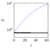
(a)

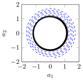
(b)

(c)

Figure 1: Nonlinear model reduction of the laminar airfoil. Evolution of modal energy (a), and phase plot of the first and second temporal basis, $a_{1}(t)$ and $a_{2}(t)$ (b); DNS (thick gray line), standard $n=4$ ROM (dashed blue line), stabilized $n,p=4$ ROM (solid black line). Stabilizing rotation matrix, $\bm{X}$ (c)

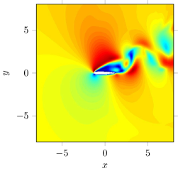
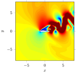
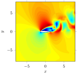
Figure 2: Snapshot of high angle of attack airfoil at final snapshot; contours of velocity magnitude. DNS (top), standard $n=4$ ROM (middle), and stabilized $n,p=4$ ROM (bottom)

4.2 Channel driven laminar cavity

For the results presented in this section, the high-fidelity fluid simulation data are generated using a Sandia National Laboratories’ in-house finite volume flow solver known as SIGMA CFD. This code is derived from LESLIE3D [40], a Large Eddy Simulations (LES) flow solver originally developed in the Computational Combustion Laboratory at the Georgia Institute of Technology. The code has LES as well as DNS capabilities. For the channel driven laminar cavity problem considered here, the code was run in DNS mode. For a detailed description of the schemes and models implemented within LESLIE3D, the reader is referred to [15, 16].

ROMs for the channel driven laminar cavity problem are constructed using a Sandia in-house parallel C++ model reduction code known as Spirit, which constructs ROMs for compressible flow problems using the POD and continuous projection method. This code, detailed in [22], reads in the snapshot and mesh data written by a high-fidelity flow solver, creates a finite element representation of the snapshots and computes the numerical quadrature necessary for evaluation of the inner products arising in the Galerkin projection step of the model reduction. All calculations are performed in parallel using distributed matrix and vector data structures and parallel eigensolvers from the Trilinos project [18], which allows for large data sets and a relatively large number of POD modes. The libmesh finite element library [24] is used to compute the element quadratures.

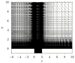
Figure 3: Domain and mesh for viscous channel driven cavity problem

In the discussion that follows, two variants of the 2D channel driven laminar cavity problem are considered: a low Reynolds number variant (${\rm Re}\approx 1500$) and a moderate Reynolds number variant (${\rm Re}\approx 5500$). Both tests cases involve a Mach 0.6 viscous laminar flow over a cavity in a $T$–shaped domain (Figure 3). The flow conditions for both tests are similar to case L2 in [36]. The free stream pressure is $25$ Pa, the free stream temperature is $300$ K, and the free stream velocity is $208.8$ m/s. The viscosity $\mu$ is spatially constant and calculated such that the above Reynolds numbers are achieved. The thermal conductivity $\kappa$ is also constant, calculated such that the Prandtl number is Pr$=0.72$. At the inflow boundary, a value of the velocity and temperature that is above the free stream values is specified. The flow at the cavity walls is assumed to be adiabatic and to satisfy a no-slip condition. The remaining outflow boundaries are open, and a far-field boundary condition that suppresses the reflection of waves into the computational domain is implemented here. The high-fidelity simulation is initialized by setting the flow in the cavity to have a zero velocity, free stream pressure, and temperature. The region above the cavity is initialized to free stream conditions and the flow is allowed to evolve. As both SIGMA CFD and Spirit are 3D codes, a 2D mesh of the domain $\Omega$ is converted to a 3D mesh by extruding the 2D mesh in the $z$-direction by one element. Finally, it is noted that SIGMA CFD and Spirit work with different meshes. The former code requires a structured hexahedral discretization, whereas the latter assumes a tetrahedral discretization. To overcome this difference, the hexahedral high-fidelity meshes associated with the snapshots are converted to tetrahedral meshes prior to constructing the ROMs. This is accomplished by breaking up each hexahedral element into six tetrahedral elements.

4.2.1 Low Reynolds number $({\rm Re}\approx 1500)$

For the first, low Reynolds number variant of the channel driven laminar cavity problem, the free-stream viscosity is set to $\mu_{\infty}=3.17\times 10^{-6}$ kg/(m$\cdot$s), so that ${\rm Re}=1453.9$. The discretized domain, illustrated in Figure 3, consists of 98,408 nodes, cast as 292,500 tetrahedral finite elements within the ROM code, Spirit. The 2D extent of the domain is: $[(-6.42,10)\times(-1,10)]\backslash[(-6.42,10)\times(-1,0)\cup(2,10)\times(-1,0)]$ m. The reader can observe that the mesh is structured but non-uniform.

The high-fidelity solver, SIGMA CFD, is initiated with the conditions described above and allowed to run until a statistically stationary flow regime is reached. At this point, a total of $K_{max}=500$ snapshots are collected from SIGMA CFD, taken every $\Delta t_{snap}=1\times 10^{-4}$ seconds. The snapshots are used to construct a POD basis of size 4 modes in the $L^{2}$ inner product. This basis captured about 91% of the snapshot energy. For more details on this test case, the reader is referred to [22].

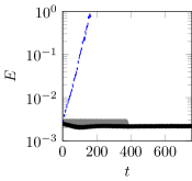
(a)

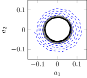
(b)

(c)

Figure 4: Nonlinear model reduction of channel drive cavity at ${\rm Re}\approx 1500$. Evolution of modal energy (a) and phase plot of the first and second temporal basis, $a_{1}(t)$ and $a_{2}(t)$ (b); DNS (thick gray line), standard $n=4$ ROM (dashed blue line), stabilized $n,p=4$ ROM (solid black line). Stabilizing rotation matrix, $\bm{X}$ (c)

Figure 4 illustrates the performance of a stabilized $n,p=4$ ROM of the low Reynolds number cavity. In Figure 4(b), the modal energy of the DNS, standard, and stabilized ROMs are illustrated. The stabilized ROM is shown to track very accurately the energy of the original DNS snapshots while the standard ROM is unable to reproduce this trajectory. The long term stability of the stabilized ROM was validated by numerically integrating the system $100\times$ the duration of the original snapshots. No change or drift in trajectory was observed during this long integration period. In Figure 4(b) the trajectories of the first and second temporal coefficient, $a_{1}(t),$ and $a_{2}(t)$ respectively, are illustrated. The stabilized ROM predicts correctly the closed orbit of the stable limit cycle while the standard ROM predicts an unstable spiral. The stabilizing transformation matrix $\bm{X}$ for this problem is illustrated Figure 4(c). As before, the rotation of the projection subspace is small as demonstrated by the fact that $\bm{X}\approx\bm{I}_{(n+p)\times n}$. For this configuration, the normalized error defined as $||\bm{X}-\bm{I}_{(n+p)\times n}||_{F}/n$ is $0.1182$.

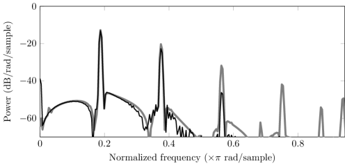
Figure 5: PSD of $p(\bm{x},t)$ where $x=(2,-1)$ of channel drive cavity ${\rm Re}\approx 1500$. DNS (thick gray line), stabilized $n,p=4$ ROM (black line)

Figure 5 shows the Power Spectral Density (PSD) of the predicted pressure fluctuations at the bottom right corner of the cavity, $\bm{x}=(2,-1)$, Both the fundamental and first harmonic of the response is accurately predicted by the stabilized $n,p=4$ ROM. The PSD of the CFD signal was computed using all available snapshots from $t=0$ to $t=380$ where $t$ is non-dimensional. On the other hand, the PSD of the stabilized ROM was computed from the signal $100\times$ past the duration of the original snapshots; i.e. $t=(38000-380)$ to $t=38000$.

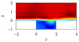
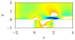
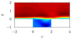
Figure 6: Snapshot of channel drive cavity ${\rm Re}\approx 1500$; contours of $u$-velocity magnitude at the final snapshot. DNS (top), standard $n=4$ ROM (middle) and stabilized $n,p=4$ ROM (bottom)

Finally, a snapshot of the predicted velocity magnitude at the final snapshot is illustrated in Figure 6. The stabilized ROM (Figure 6(a)) reproduces the velocity contours of the original high-fidelity DNS simulation (Figure 6(c)) remarkably well. In contrast, the standard ROM (Figure 6(c)) is unstable and inaccurate.

4.2.2 Moderate Reynolds number $({\rm Re}\approx 5500)$

The next test case considered is also a channel drive laminar cavity problem, but at a higher Reynolds number. The only parameter that is different is the free-stream viscosity, now set to $\mu_{\infty}=8.46\times 10^{-7}$ kg/(m$\cdot$s), so that ${\rm Re}=5452.1$. Also changed is the size of the geometry extent, which has a larger sponge region near the outflow regions. This is needed to suppress adequately the reflection of waves into the computational domain for this problem. Toward this effect, the 2D extent of the domain is: $[(-6.42,30)\times(-1,30)]\backslash[(-6.42,30)\times(-1,0)\cup(2,30)\times(-1,0)]$ m. The geometry is discretized by 117,328 nodes, cast as 345,900 tetrahedral elements in Spirit. As before, the mesh is structured but non-uniform. The flow is significantly more chaotic than the ${\rm Re}\approx 1500$ case considered in Section 4.2.1.

A total of $K=500$ snapshots are collected from SIGMA CFD at increments $\Delta t_{snap}=1\times 10^{-5}$ seconds. As before, snapshots collection does not begin until a statistically stationary flow regime has been reached. From these snapshots, a POD basis of size 20 modes is constructed in the $L^{2}$ inner product. This basis captures about 72% of the snapshot energy. Typically, $n$ would be selected such that the POD basis captures a greater percentage of the snapshot ensemble energy (e.g., $\approx 90\%$ or more). We choose a basis that captures less energy of the snapshot set to highlight the effectiveness of our approach for low-dimensional POD expansions.

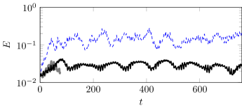
(a)

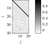
(b)

Figure 7: Nonlinear model reduction of channel drive cavity at ${\rm Re}\approx 5500$. Evolution of modal energy (a); DNS (thick gray line), standard $n=20$ ROM (dashed blue line), stabilized $n,p=20$ ROM (solid black line). Stabilizing rotation matrix, $\bm{X}$ (b)

Figure 7 illustrates the performance of a stabilized $n,p=20$ ROM of the higher Reynolds number cavity problem. In Figure 7(a), the modal energy of the DNS, standard, and stabilized ROMs are illustrated. The standard ROM is shown to over predict the energy of the original DNS snapshots by an order of magnitude. The predictive power of the stabilized ROM is demonstrated by numerically integrating the ROM $10\times$ the duration of the original snapshots. The stabilizing transformation matrix $\bm{X}$ for this problem is illustrated Figure 7(b). As before, the rotation of the projection subspace is small as demonstrated by the fact that $\bm{X}\approx\bm{I}_{(n+p)\times n}$. For this configuration, the normalized error defined as $||\bm{X}-\bm{I}_{(n+p)\times n}||_{F}/n$ is $0.0384$.

Figures 8 and 9 shows the PSDs of the predicted pressure fluctuations at locations $\bm{x}_{1}=(2,-0.5)$ and $\bm{x}_{2}=(2,0.5)$, respectively. The PSD of the CFD signal was computed using all available snapshots from $t=0$ to $t=67$ where $t$ is non-dimensional. On the other hand, the PSD of the stabilized ROM was computed from the signal $10\times$ past the duration of the original snapshots; i.e. $t=(670-67)$ to $t=670$. The stabilized ROM accurately predicts the chaotic pressure fluctuations at both locations. Figure 10 illustrates the Cross Power Spectral Density (CPSD) for pressure fluctuations at $\bm{x}_{1}$ and $\bm{x}_{2}$. Both the power and phase lag at the fundamental frequency, and the first two super harmonics (normalized frequency ($\times\pi$ rad/sample) $\approx 0.18,0.35,$ and $0.53$) are predicted accurately using the stabilized ROM. The phase lag at these three frequencies in Figure 10 as predicted by the CFD and the stabilized ROM is identified by red squares and blue triangles, respectively. As expected, the low-dimensional ROM is unable to reproduce the phase lag of low-amplitude frequencies or higher-order super harmonics. Finally, a snapshot of the predicted velocity and pressure magnitudes at the final snapshot are illustrated in Figure 11 and 12. Since the flow at this higher Reynolds number is chaotic, the low-dimensional model can not be expected to track the original snapshots exactly. However, the snapshots demonstrates that the stabilized ROMs faithfully reproduce the large features of the flow. The same cannot be said of the standard ROMs.

4.3 Computational speed-up

For each problem considered, the speed-up factor delivered by its ROM for the online computations is reported in Table 1. All ROMs are solved in MATLAB using the variable order solver ODE15s; Jacobians are provided analytically. For more details on this algorithm, the reader is referred to Shampine et al. [43]. All online time-integration CPU times were measured using the tic-toc function on a single computational thread via the -singleCompThread start-up option. The FOM time-integration, basis construction and Galerkin projection times given in the table are reported in CPU-hours, calculated as the product of the number of processors used in the computation and the mean CPU time over all processors. The number of processors employed varied between 1 and 128. The online speed-up is calculated by evaluating the ratio between the time-integration of the FOM and the time-integration of the ROM. The reader can observe that the ROM online speedup is on the order of at least $10^{4}$ for all three problems considered. Moreover, the stabilization step takes very little time (on the order of seconds/minutes).

Table 1: CPU times for off-line and on-line computations.

	Numerical Experiment
Procedure	Airfoil	Cavity, Low-Re	Cavity, Moderate-Re
FOM # of DOF	360,000	288,250	243,750
Time-integration of FOM	7.8 hrs	72 hrs	179 hrs
Basis construction (size $n+p$ ROM)	0.16 hrs	0.88 hrs	3.44 hrs
Galerkin projection (size $n+p$ ROM)	0.74 hrs	5.44 hrs	14.8 hrs
Stabilization	28 sec	14 sec	170 sec
ROM # of DOF	4	4	20
Time-integration of ROM	0.31 sec	0.16 sec	0.83 sec
Online computational speed-up	$9.1\times 10^{4}$	$1.6\times 10^{6}$	$7.8\times 10^{5}$

5 Conclusions

In this paper, an approach for stabilizing and enhancing projection-based fluid ROMs of the compressible Navier-Stokes equations is developed. Unlike traditional approaches, no empirical turbulence modeling terms are required, and consistency between the ROM and the full order model from which the ROM is derived is maintained. Mathematically, the approach is formulated as a trace minimization on the Stiefel manifold. The method is shown to yield both stable and accurate low-dimensional models of several representative compressible flow problems. In particular, the method is demonstrated on flows at higher Reynolds number where the dynamics are chaotic. Future work will include the extension of the proposed approach to problems with generic non-linearities, where the ROM involves some form of hyper-reduction (e.g., DEIM, gappy POD) following the procedure described in Remark 2, as well as to predictive applications with varying Reynolds number and geometry.

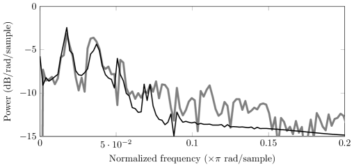
Figure 8: PSD of $p(\bm{x}_{1},t)$ where $\bm{x}_{1}=(2,-0.5)$ of channel driven cavity at ${\rm Re}\approx 5500$. DNS (thick gray line), stabilized $n,p=20$ ROM (black line)

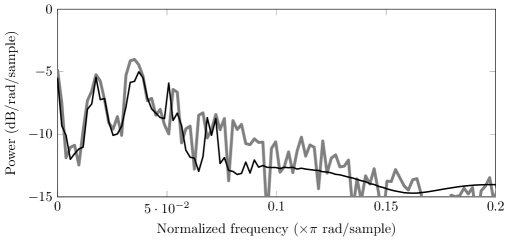
Figure 9: PSD of $p(\bm{x}_{2},t)$ where $\bm{x}_{2}=(0,-0.5)$ of channel driven cavity at ${\rm Re}\approx 5500$. DNS (thick gray line), stabilized $n,p=20$ ROM (black line)

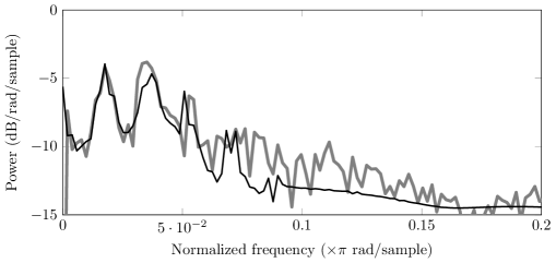
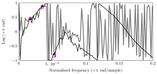
Figure 10: CPSD of $p(\bm{x}_{1},t)$ and $p(\bm{x}_{2},t)$ where $\bm{x}_{1}=(2,-0.5)$ and $\bm{x}_{2}=(0,-0.5)$ of channel driven cavity at ${\rm Re}\approx 5500$. DNS (thick gray line), stabilized $n,p=20$ ROM (black line)

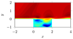
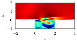
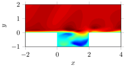
Figure 11: Snapshot of channel drive cavity ${\rm Re}\approx 5500$; contours of $u$-velocity magnitude at the final snapshot. DNS (top), standard $n=20$ ROM (middle), and stabilized $n,p=20$ ROM (bottom)

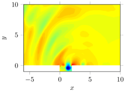
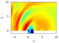
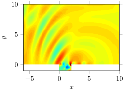
Figure 12: Snapshot of channel driven cavity ${\rm Re}\approx 5500$; contours of pressure at the final snapshot. DNS (top), standard $n=20$ ROM (middle), and stabilized $n,p=20$ ROM (bottom)

Appendix A Construction of Galerkin matrices for the compressible Navier-Stokes equations

In this section the construction of Galerkin matrices for the compressible Navier-Stokes equations (6) is outlined. Consider the standard orthonormal POD vectors $u^{i}$, $v^{i}$, $\zeta^{i}$, and $p^{i}$, $i=0,\cdots,n$ where $i=0$ identifies the constant mean flow. The following products are generated for $j,k=0,\cdots,n$:

$$\phi_{1}^{(j,k)} =u^{j}\odot\zeta_{x}^{k}+v^{j}\odot\zeta_{y}^{k}-u_{x}\odot\zeta^{k}-v_{y}^{j}\odot\zeta^{k},$$ (19a)

$$\phi_{2}^{(j,k)} =u^{j}\odot u_{x}^{k}+v^{j}\odot u_{y}^{k}+\zeta^{j}\odot p_{x}^{k}-\frac{1}{{\rm Re}}\zeta^{j}\odot\left[\left(\frac{4}{3}u_{x}^{k}-\frac{2}{3}v_{y}^{k}\right)_{x}+(v_{x}^{k}+u_{y}^{k})_{y}\right],$$ (19b)

$$\phi_{3}^{(j,k)} =u^{j}\odot v_{x}^{k}+v^{j}\odot v_{y}^{k}+\zeta^{j}\odot p_{y}^{k}-\frac{1}{{\rm Re}}\zeta^{j}\odot\left[\left(\frac{4}{3}v_{y}^{k}-\frac{2}{3}u_{x}^{k}\right)_{y}+(v_{x}^{k}+u_{y}^{k})_{x}\right],$$ (19c)

$$\begin{split}\phi_{4}^{(j,k)}&=u^{j}\odot p_{x}^{k}+v^{j}\odot p_{y}^{k}+\gamma p^{j}\odot(v_{x}^{k}+u_{y}^{k})-\frac{\gamma}{{\rm Re}\,{\rm Pr}}\left[(p^{j}\odot\zeta_{k})_{xx}+(p^{j}\odot\zeta_{k})_{yy}\right]\\ &+\frac{1-\gamma}{{\rm Re}}\left[u_{x}^{j}\odot\left(\frac{4}{3}u_{x}^{k}-\frac{2}{3}v_{y}^{k}\right)+v_{y}^{j}\odot\left(\frac{4}{3}v_{y}^{k}-\frac{2}{3}u_{x}^{k}\right)+(u_{y}^{j}+v_{x}^{j})\odot(u_{y}^{k}+v_{x}^{k})\right],\end{split}$$ (19d)

where subscripts identify partial spatial derivatives, and $\odot$ is the Hadamard element-by-element product. A standard $L^{2}$ Galerkin projection for $i,j,k=0,\cdots,n$ is performed as follows:

$$b^{(i)}(j,k)=\sum_{m=0}^{N}\left[h\odot\left(\zeta^{i}\odot\phi_{1}^{(j,k)}+u^{i}\odot\phi_{2}^{(j,k)}+v^{i}\odot\phi_{3}^{(j,k)}+p^{i}\odot\phi_{4}^{(j,k)}\right)\right]_{m},$$ (20)

where $h$ is a vector of element volumes. Finally, the standard Galerkin matrices for $i,j,k=1,\cdots,n$ with $a_{0}=1$, are given by

$$C_{i} =b^{(i)}(0,0),$$ (21a)

$$L_{i,j} =b^{(i)}(j,0)+b^{(i)}(0,j),$$ (21b)

$$Q^{(i)}_{j,k} =b^{(i)}(j,k).$$ (21c)

References

- Amsallem and Farhat [2012] Amsallem, D., Farhat, C., 2012. Stabilization of projection-based reduced-order models. International Journal for Numerical Methods in Engineering 91 (4), 358–377.
- Aubry et al. [1988] Aubry, N., Holmes, P., Lumley, J. L., Stone, E., 1988. The dynamics of coherent structures in the wall region of a turbulent boundary layer. Journal of Fluid Mechanics 192, 115–173.
- Balajewicz and Dowell [2012] Balajewicz, M., Dowell, E. H., 2012. Stabilization of projection-based reduced order models of the Navier–Stokes. Nonlinear Dynamics 70 (2), 1619–1632.
- Balajewicz and Farhat [2014] Balajewicz, M., Farhat, C., 2014. Reduction of nonlinear embedded boundary models for problems with evolving interfaces. Journal of Computational Physics 274, 489–504.
- Balajewicz et al. [2013] Balajewicz, M. J., Dowell, E. H., Noack, B. R., 2013. Low-dimensional modelling of high-Reynolds-number shear flows incorporating constraints from the Navier–Stokes equation. Journal of Fluid Mechanics 729, 285–308.
- Barone [2015] Barone, M. F., 2015. Survey of model reduction methods for compressible flows (in preparation). Tech. rep., Sandia National Laboratories, Albuquerque, NM.
- Barone et al. [2009] Barone, M. F., Kalashnikova, I., Segalman, D. J., Thornquist, H. K., 2009. Stable galerkin reduced order models for linearized compressible flow. Journal of Computational Physics 228 (6), 1932–1946.
- Boumal et al. [2014] Boumal, N., Mishra, B., Absil, P. A., Sepulchre, R., 2014. Manopt, a Matlab toolbox for optimization on manifolds. Journal of Machine Learning Research 15, 1455–1459.
- Bui-Thanh et al. [2007] Bui-Thanh, T., Willcox, K., Ghattas, O., van Bloemen Waanders, B., 2007. Goal-oriented, model-constrained optimization for reduction of large-scale systems. Journal of Computational Physics 224 (2), 880–896.
- Carlberg et al. [2013] Carlberg, K., Farhat, C., Cortial, J., Amsallem, D., 2013. The GNAT method for nonlinear model reduction: effective implementation and application to computational fluid dynamics and turbulent flows. Journal of Computational Physics 242, 623–647.
- Carlberg et al. [2015] Carlberg, K., Tuminaro, R., Boggs, P., 2015. Preserving Lagrangian structure in nonlinear model reduction with application to structural dynamics. SIAM J. Sci. Comput. 47 (2) B153–B184.
- Cazemier et al. [1998] Cazemier, W., Verstappen, R. W. C. P., Veldman, A. E. P., 1998. Proper orthogonal decomposition and low-dimensional models for driven cavity flows. Physics of Fluids (1994-present) 10 (7), 1685–1699.
- Eckart and Young [1936] Eckart, C., Young, G., 1936. The approximation of one matrix by another of lower rank. Psychometrika 1 (3), 211–218.
- Galletti et al. [2004] Galletti, B., Bruneau, C. H., Zannetti, L., Iollo, A., 2004. Low-order modelling of laminar flow regimes past a confined square cylinder. Journal of Fluid Mechanics 503, 161–170.
- Génin and Menon [2010a] Génin, F., Menon, S., 2010a. Dynamics of sonic jet injection into supersonic crossflow. Journal of Turbulence 11 (4), 1–30.
- Génin and Menon [2010b] Génin, F., Menon, S., 2010b. Studies of shock/turbulent shear layer interaction using large-eddy simulation. Computers & Fluids 39 (5), 800–819.
- Gugercin and Antoulas [2004] Gugercin, S., Antoulas, A. C., 2004. A survey of model reduction by balanced truncation and some new results. International Journal of Control 77 (8), 748–766.
- Heroux et al. [2005] Heroux, M. A., Bartlett, R. A., Howle, V. E., Hoekstra, R. J., Hu, J. J., Kolda, T. G., Lehoucq, R. B., Long, K. R., Pawlowski, R. P., Phipps, E. T., Salinger, A. G., Thornquist, H. K., Tuminaro, R. S., Willenbring, J. M., Williams, A., Stanley, K. S., 2005. An overview of the trilinos project. ACM Transactions on Mathematical Software (TOMS) 31 (3), 397–423.
- Holmes et al. [2012] Holmes, P., Lumley, J. L., Berkooz, G., Rowley, C. W., 2012. Turbulence, coherent structures, dynamical systems and symmetry, 2nd Edition. Cambridge university press.
- Iliescu and Wang [2014] Iliescu, T., Wang, Z., 2014. Variational multiscale proper orthogonal decomposition: Navier-stokes equations. Numerical Methods for Partial Differential Equations 30 (2), 641–663.
- Iollo et al. [2000] Iollo, A., Lanteri, S., Désidéri, J., 2000. Stability properties of POD–Galerkin approximations for the compressible Navier–Stokes equations. Theoretical and Computational Fluid Dynamics 13 (6), 377–396.
- Kalashnikova et al. [2014a] Kalashnikova, I., Arunajatesan, S., Barone, M. F., van Bloemen Waanders, B. G., Fike, J. A., 2014a. Reduced order modeling for prediction and control of large-scale systems. Tech. rep., Sandia National Laboratories, Albuquerque, NM.
- Kalashnikova et al. [2014b] Kalashnikova, I., van Bloemen Waanders, B., Arunajatesan, S., Barone, M., 2014b. Stabilization of projection-based reduced order models for linear time-invariant systems via optimization-based eigenvalue reassignment. Computer Methods in Applied Mechanics and Engineering 272, 251–270.
- Kirk et al. [2006] Kirk, B. S., Peterson, J. W., Stogner, R. H., Carey, G. F., 2006. libmesh: a c++ library for parallel adaptive mesh refinement/coarsening simulations. Engineering with Computers 22 (3-4), 237–254.
- Lumley [1971] Lumley, J. L., 1971. Stochastic tools in turbulence. Academic Press: New York.
- Mirsky [1960] Mirsky, L., 1960. Symmetric gauge functions and unitarily invariant norms. Quarterly Journal of Mathematics 11, 50–59.
- Moore [1981] Moore, B., 1981. Principal component analysis in linear systems: Controllability, observability, and model reduction. Automatic Control, IEEE Transactions on 26 (1), 17–32.
- Noack et al. [2008] Noack, B. R., Schlegel, M., Ahlborn, B., Mutschke, G., Morzyński, M., Comte, P., 2008. A finite-time thermodynamics of unsteady fluid flows. Journal of Non-Equilibrium Thermodynamics 33 (2), 103–148.
- Nocedal [1999] Nocedal, J., 1999. Numerical Optimization. Springer.
- Östh et al. [2014] Östh, J., Noack, B. R., Krajnović, S., Barros, D., Borée, J., 2014. On the need for a nonlinear subscale turbulence term in POD models as exemplified for a high-Reynolds-number flow over an ahmed body. Journal of Fluid Mechanics 747, 518–544.
- Pope [2000] Pope, S. B., 2000. Turbulent flows, 6th Edition. Cambridge university press.
- Protas et al. [2014] Protas, B., Noack, B. R., Östh, J., 2014. Optimal nonlinear eddy viscosity in galerkin models of turbulent flows. arXiv preprint arXiv:1406.1912.
- Rapcsák [2002] Rapcsák, T., 2002. On minimization on stiefel manifolds. European Journal of Operational Research 143 (2), 365–376.
- Rempfer and Fasel [1994] Rempfer, D., Fasel, H. F., 1994. Dynamics of three-dimensional coherent structures in a flat-plate boundary layer. Journal of Fluid Mechanics 275, 257–283.
- Rowley [2005] Rowley, C. W., 2005. Model reduction for fluids, using balanced proper orthogonal decomposition. International Journal of Bifurcation and Chaos 15 (03), 997–1013.
- Rowley et al. [2002] Rowley, C. W., Colonius, T., Basu, A. J., 2002. On self-sustained oscillations in two-dimensional compressible flow over rectangular cavities. Journal of Fluid Mechanics 455, 315–346.
- Rowley et al. [2004] Rowley, C. W., Colonius, T., Murray, R. M., 2004. Model reduction for compressible flows using pod and Galerkin projection. Physica D: Nonlinear Phenomena 189 (1), 115–129.
- Rowley et al. [2009] Rowley, C. W., Mezić, I., Bagheri, S., Schlatter, P., Henningson, D. S., 2009. Spectral analysis of nonlinear flows. Journal of Fluid Mechanics 641, 115–127.
- Rozza [2011] Rozza, G., 2011. Reduced basis approximation and error bounds for potential flows in parametrized geometries. Communication in Computational Physics 9, 1–48.
- Sankaran and Menon [2005] Sankaran, V., Menon, S., 2005. Les of scalar mixing in supersonic mixing layers. Proceedings of the combustion Institute 30 (2), 2835–2842.
- Schmid [2010] Schmid, P. J., 2010. Dynamic mode decomposition of numerical and experimental data. Journal of Fluid Mechanics 656, 5–28.
- Serre et al. [2012] Serre, G., Lafon, P., Gloerfelt, X., Bailly, C., 2012. Reliable reduced-order models for time-dependent linearized euler equations. Journal of Computational Physics 231 (15), 5176–5194.
- Shampine et al. [1997] Shampine, L., Reichelt, M., 1997. The MATLAB ODE suite. SIAM Journal of Scientific Computing 18 (1), 1–22.
- Sirovich [1987] Sirovich, L., 1987. Turbulence and the dynamics of coherent structures. Part III: dynamics and scaling. Quarterly of applied mathematics 45 (3), 583–590.
- Stiefel [1935] Stiefel, E., 1935. Richtungsfelder und fernparallelismus in n-dimensionalen mannigfaltigkeiten. Commentarii Mathematici Helvetici 8 (1), 305–353.
- Tennekes and Lumley [1972] Tennekes, H., Lumley, J. L., 1972. A first course in turbulence. MIT press.
- Veroy and Patera [2005] Veroy, K., Patera, A. T., 2005. Certified real-time solution of the parametrized steady incompressible navier–stokes equations: rigorous reduced-basis a posteriori error bounds. International Journal for Numerical Methods in Fluids 47 (8-9), 773–788.
- Wang et al. [2012] Wang, Z., Akhtar, I., Borggaard, J., Iliescu, T., 2012. Proper orthogonal decomposition closure models for turbulent flows: a numerical comparison. Computer Methods in Applied Mechanics and Engineering 237, 10–26.
- Willcox and Peraire [2002] Willcox, K., Peraire, J., 2002. Balanced model reduction via the proper orthogonal decomposition. AIAA journal 40 (11), 2323–2330.