NCTS-TH/1502

Inflation from radion gauge-Higgs potential
at Planck scale

Yugo Abe^a, Takeo Inami^b, Yoshiharu Kawamura^a and Yoji Koyama^c

${}^{a}\,$Department of Physics, Shinshu University, Matsumoto 390-8621, Japan
${}^{b}\,$Mathematical Physics Lab., Riken Nishina Center, Saitama, Japan
${}^{b}\,$Department of Physics, National Taiwan University, Taipei, Taiwan
${}^{c}\,$National Center for Theoretical Science, Hsinchu, Taiwan 300

We study whether the inflation is realized based on the radion gauge-Higgs potential obtained from the one-loop calculation in the 5-dimensional gravity coupled to a $U(1)$ gauge theory. We show that the gauge-Higgs can give rise to inflation in accord with the astrophysical data and the radion plays a role in fixing the values of physical parameters. We clarify the reason why the radion dominated inflation and the hybrid inflation cannot occur in our framework.

1 Introduction

It is believed that the universe has evolved into the present one as a result of a rapid expansion called $``$inflation” in its very early stage. The well-known difficulties in the standard big-bang model are solved by the slow-roll inflation scenario [1, 2]. Furthermore recent accurate measurements have confirmed the predictions of a flat universe with a nearly scale-invariant density perturbation [3].

A remaining big problem is to explore the origin of inflation or to disclose the identity of a scalar particle called $``$inflaton”. The following requirements can be imposed on the model as clues to a solution. The inflaton should be the inevitable product of a theory at a high-energy scale. The potential of inflaton should be stable against various corrections. Concretely, there should be no fine tuning among parameters receiving quantum corrections and no sensitivity to gravitational corrections.

On a 4-dimensional (4D) space-time, no model has yet been known to solve the problem completely. In most models, the inflaton is an ad-hoc particle introduced by hand, and the stability of potential is threatened by radiative corrections and gravitational ones relating non-renormalizable terms suppressed by the power of the Planck mass because the inflaton takes a larger value than the Planck mass and such corrections cannot be controlled without any powerful symmetries and/or mechanisms.

Effective field theories on a higher-dimensional space-time provide a possible solution to the problem. Some scalar fields exist inevitably as parts of ingredients in the theory and are massless at the tree level. The scalar potential can be induced radiatively and stabilized by local symmetries. Typical ones are the extranatural inflation model [4, 5] and the radion inflation model [6]. In the former model, a scalar field called $``$gauge-Higgs” appears from the extra-dimensional component(s) of the gauge field. It becomes dynamical degrees of freedom called the Wilson line phase and its value is fixed by quantum corrections [7]. In the latter model, a scalar field called $``$radion” originates from the extra-dimensional component(s) of the graviton, and its vacuum expectation value (VEV) is related to the size of the extra space.

Recently, the effective potential with respect to both the radion and the gauge-Higgs has been derived at the one-loop level upon the $S^{1}$ compactification, from the gravity theory coupled to a $U(1)$ gauge boson and matter fermions on a 5-dimensional (5D) space-time [8]. We refer to the potential as the $``$radion gauge-Higgs potential”. It is interesting to investigate whether it works as the inflaton potential and what features exist in such a coexisting system.

In this article, we study whether the slow-roll inflation is realized compatible with the astrophysical data, based on the radion gauge-Higgs potential. In the analysis, we pay attention to which particle can play the role of inflaton and the magnitude of physical parameters.

The content of our article is as follows. In the next section, we explain the radion gauge-Higgs potential and constraints on the inflaton potential. In Sect. 3, we study the gauge-Higgs inflation after focusing on a candidate of inflaton. It will be shown that the inflation can be achieved in our framework. In the last section, we give conclusions and discussions.

2 Setup

2.1 Radion gauge-Higgs potential

Based on a 5D theory containing a graviton, a $U(1)$ gauge boson and fermions, the following radion gauge-Higgs potential have been obtained at the one-loop level [8],

$$V(\chi,\varphi)=\frac{3}{\pi^{2}\chi^{2}L^{4}}\left[-2\zeta(5)+c_{1}\sum^{\infty}_{k=1}\left(\frac{1}{k^{5}}+r_{m}\frac{Lm\chi^{1/3}}{k^{4}}+r^{2}_{m}\frac{L^{2}m^{2}\chi^{2/3}}{3k^{3}}\right)e^{-kr_{m}Lm\chi^{1/3}}~{}~{}~{}~{}~{}~{}~{}\right.$$

$$~{}~{}~{}~{}~{}\left.+c_{2}\sum^{\infty}_{k=1}\left(\frac{1}{k^{5}}+\frac{Lm\chi^{1/3}}{k^{4}}+\frac{L^{2}m^{2}\chi^{2/3}}{3k^{3}}\right)e^{-kLm\chi^{1/3}}\cos{(kg_{4}L\varphi)}\right]+aL\chi^{-1/3}+\cdots~{},$$ (2.1)

where $\chi$ is the radion, $\varphi$ the gauge-Higgs, $L$ the $S^{1}$ circumference, $g_{4}$ the 4D gauge coupling constant, $c_{1}$ and $c_{2}$ the numbers of neutral and charged fermions whose masses are $\mu$ and $m$, $r_{m}=\mu/m$ and the ellipsis stands for terms including infinities whose form is consistent with the general covariance, e.g. $\Lambda^{5}L\chi^{-1/3}$ with $\Lambda$ the UV cutoff. Using $r_{m}$, we can control contributions of two kinds of fermions to the potential through the factor $e^{-kr_{m}Lm\chi^{1/3}}$. Note that the 5D cosmological constant counter term $aL\chi^{-1/3}$ is introduced to remove infinities [9, 10].

The stabilization of $\chi$ and $\varphi$ has been studied and it has been shown that the potential has a stable minimum if $c_{1}>c_{2}+2$. The physical length of the 5-th dimension $L_{\rm phys}$, the physical fermion masses $m_{\rm phys}$ and $\mu_{\rm phys}$ are given by

$$L_{\rm phys}=L\langle\chi\rangle^{1/3}~{},~{}~{}m_{\rm phys}=m\langle\chi\rangle^{-1/6}~{},~{}~{}\mu_{\rm phys}=r_{m}m_{\rm phys}~{},$$ (2.2)

where $\langle\chi\rangle$ is the VEV of $\chi$ at the minimum of $V$.

It is an attractive idea that the structure and evolution of our 4D space-time might be deeply linked to the dynamics of quantities relating an extra space. The $V(\chi,\varphi)$ must describe the physics around the Planck scale if the magnitude of $L_{\rm phys}^{-1}$, $m_{\rm phys}$ and/or $\mu_{\rm phys}$ can be comparable to the reduced Planck mass $M_{G}$ ($\equiv(8\pi G)^{-1/2}=2.4\times 10^{18}$GeV). There are nearly flat domains around the minimum of $V(\chi,\varphi)$. Hence it is reasonable to expect that the radion gauge-Higgs potential plays the role of inflaton potential.

2.2 Constraints on inflaton potential

From the inflation theory and the observational data, we have several constraints on the inflaton potential $V$ [1, 3]. Leading constraints are listed as

$$\cdot {\rm the~{}slow\mathchar 45\relax roll~{}parameters}~{}~{}~{}~{}~{}~{}~{}~{}\epsilon\equiv\frac{1}{2}M^{2}_{G}\left(\frac{V^{\prime}}{V}\right)^{2}\ll 1~{},~{}~{}~{}\eta~{}\equiv~{}M^{2}_{G}\frac{V^{\prime\prime}}{V}\ll 1~{},$$ (2.3)

$$\cdot {\rm the~{}spectral~{}index}~{}~{}~{}~{}~{}~{}~{}~{}~{}~{}~{}~{}~{}~{}~{}~{}n_{s\ast}\equiv 1-6\epsilon_{\ast}+2\eta_{\ast}=0.9655\pm 0.0062~{},$$ (2.4)

$$\cdot {\rm the~{}number~{}of~{}e\mathchar 45\relax foldings}~{}~{}~{}~{}~{}~{}~{}N\equiv\frac{1}{M^{2}_{G}}\left|\int^{\phi_{e}}_{\phi_{\ast}}\frac{V}{V^{\prime}}d\phi\right|=50\sim 60~{},$$ (2.5)

$$\cdot {\rm the~{}scalar~{}power~{}spectrum}~{}~{}~{}~{}~{}{\mathcal{P}}_{\zeta\ast}\equiv\left.\frac{1}{12\pi^{2}M^{6}_{G}}\frac{V^{3}}{(V^{\prime})^{2}}\right|_{\phi=\phi_{\ast}}\!\!\!\!\!=(2.196\pm 0.079)\times 10^{-9},$$ (2.6)

$$\cdot {\rm the~{}tensor\mathchar 45\relax to\mathchar 45\relax scalar~{}ratio}~{}~{}~{}~{}~{}~{}~{}r=16\epsilon_{\ast}<0.12~{},$$ (2.7)

$$\cdot {\rm the~{}vacuum~{}energy}~{}~{}~{}~{}~{}~{}~{}~{}~{}~{}~{}~{}~{}~{}~{}V(\phi_{e})\cong 0~{},$$ (2.8)

where $\phi$ is the inflaton field canonically normalized with a mass dimension, $V^{\prime}=\partial V/\partial\phi$ and $V^{\prime\prime}=\partial^{2}V/\partial\phi^{2}$. The quantities at the horizon exit are indicated by $\ast$. The subscript $e$ denotes the value at the end of the slow-roll when $\epsilon\sim 1$ or $\eta\sim 1$.

Our 4D effective theory contains two scalar fields inevitably. One is the canonically normalized radion $\chi^{\prime}$ defined by

$$\chi^{\prime}\equiv\frac{M_{G}}{\sqrt{6}}\ln{\chi}~{}.$$ (2.9)

The other is the gauge-Higgs $\varphi$ given as a canonically normalized one. In the analysis of the slow-roll inflation, it is often convenient to use the dimensionless field variables such as $x(=L^{3}m^{3}\chi)$ and the Wilson line phase $\theta(=g_{4}L\varphi)$. Using them, the potential (2.1) is rewritten as

$$V(x,\theta) = \frac{3L^{2}m^{6}}{\pi^{2}x^{2}}\left[-2\zeta(5)+c_{1}\sum^{\infty}_{k=1}\left(\frac{1}{k^{5}}+r_{m}\frac{x^{1/3}}{k^{4}}+r^{2}_{m}\frac{x^{2/3}}{3k^{3}}\right)e^{-kr_{m}x^{1/3}}\right.$$ (2.10)

$$~{}~{}~{}\left.+c_{2}\sum^{\infty}_{k=1}\left(\frac{1}{k^{5}}+\frac{x^{1/3}}{k^{4}}+\frac{x^{2/3}}{3k^{3}}\right)e^{-kx^{1/3}}\cos{(k\theta)}\right]+\frac{L^{2}m}{x^{1/3}}a+\cdots~{}.$$

The constraint (2.8) means that the inflation ends at $\phi=\phi_{e}$, and it is given by the renormalization condition $V(\langle\chi\rangle,\langle\varphi\rangle)=0$ because the inflation must be terminated near the minimum of $V$. Here, $\langle\varphi\rangle$ is the VEV of $\varphi$ at the minimum of $V$.

3 Analysis

3.1 Candidate of inflaton

Let us guess the inflaton $\phi$ under the assumption that $V(x,\theta)$ is the inflaton potential. There are several possibilities. (a) $\phi$ is a mixture of $x$ and $\theta$. (b) $\phi$ is $x$ or $\theta$. In the hybrid inflation scenario [11], there is a field called $``$waterfall” $\omega$ other than $\phi$. The role of $\omega$ is to terminate the inflation induced by $\phi$, through the fall into the minimum of $V$.

The candidate of $\phi$ is focused on by the slow-roll conditions (2.3). The first and second derivatives of $V$ with respect to $\chi^{\prime}$ and $\varphi$ are given by

$$\frac{\partial V}{\partial\chi^{\prime}}=\frac{\sqrt{6}x}{M_{G}}\frac{\partial}{\partial x}V(x,\theta)=-\frac{6\sqrt{6}L^{2}m^{6}}{M_{G}\pi^{2}x^{2}}\left[\frac{\pi^{2}x^{5/3}}{18m^{5}}a-2\zeta(5)\right.$$

$$~{}~{}~{}~{}~{}~{}~{}~{}~{}~{}~{}~{}~{}~{}+c_{1}\sum^{\infty}_{k=1}\left(\frac{1}{k^{5}}+r_{m}\frac{x^{1/3}}{k^{4}}+r^{2}_{m}\frac{7x^{2/3}}{18k^{3}}+r^{3}_{m}\frac{x}{18k^{2}}\right)e^{-kr_{m}x^{1/3}}$$

$$~{}~{}~{}~{}~{}~{}~{}~{}~{}~{}~{}~{}~{}~{}\left.+c_{2}\sum^{\infty}_{k=1}\left(\frac{1}{k^{5}}+\frac{x^{1/3}}{k^{4}}+\frac{7x^{2/3}}{18k^{3}}+\frac{x}{18k^{2}}\right)e^{-kx^{1/3}}\cos{(k\theta)}\right],$$

$$\frac{\partial^{2}V}{\partial\chi^{\prime 2}}=\frac{6x}{M_{G}^{2}}\frac{\partial}{\partial x}V(x,\theta)+\frac{6x^{2}}{M_{G}^{2}}\frac{\partial^{2}}{\partial x^{2}}V(x,\theta)=\frac{72L^{2}m^{6}}{M_{G}^{2}\pi^{2}x^{2}}\left[\frac{\pi^{2}x^{5/3}}{108m^{5}}a-2\zeta(5)\right.$$

$$~{}~{}~{}~{}~{}~{}~{}~{}~{}~{}~{}~{}~{}~{}+c_{1}\sum^{\infty}_{k=1}\left(\frac{1}{k^{5}}+r_{m}\frac{x^{1/3}}{k^{4}}+r_{m}^{2}\frac{23x^{2/3}}{54k^{3}}+r_{m}^{3}\frac{5x}{54k^{2}}+r_{m}^{4}\frac{x^{4/3}}{108k}\right)e^{-kr_{m}x^{1/3}}$$

$$~{}~{}~{}~{}~{}~{}~{}~{}~{}~{}~{}~{}~{}~{}\left.+c_{2}\sum^{\infty}_{k=1}\left(\frac{1}{k^{5}}+\frac{x^{1/3}}{k^{4}}+\frac{23x^{2/3}}{54k^{3}}+\frac{5x}{54k^{2}}+\frac{x^{4/3}}{108k}\right)e^{-kx^{1/3}}\cos{(k\theta)}\right]~{},$$ (3.2)

$$\frac{\partial V}{\partial\varphi}=\frac{1}{f}\frac{\partial}{\partial\theta}V(x,\theta)=-\frac{3L^{2}m^{6}}{f\pi^{2}x^{2}}c_{2}\sum^{\infty}_{k=1}\left(\frac{1}{k^{4}}+\frac{x^{1/3}}{k^{3}}+\frac{x^{2/3}}{3k^{2}}\right)e^{-kx^{1/3}}\sin{(k\theta)}~{},$$ (3.3)

$$\frac{\partial^{2}V}{\partial\varphi^{2}}=\frac{1}{f^{2}}\frac{\partial^{2}}{\partial\theta^{2}}V(x,\theta)=-\frac{3L^{2}m^{6}}{f^{2}\pi^{2}x^{2}}c_{2}\sum^{\infty}_{k=1}\left(\frac{1}{k^{3}}+\frac{x^{1/3}}{k^{2}}+\frac{x^{2/3}}{3k}\right)e^{-kx^{1/3}}\cos{(k\theta)}~{},$$

$$\frac{\partial^{2}V}{\partial\chi^{\prime}\partial\varphi}=\frac{\sqrt{6}x}{fM_{G}}\frac{\partial^{2}}{\partial x\partial\theta}V(x,\theta)$$

$$~{}~{}~{}~{}~{}~{}~{}~{}~{}=-\frac{6\sqrt{6}L^{2}m^{6}}{fM_{G}\pi^{2}x^{2}}c_{2}\sum^{\infty}_{k=1}\left(\frac{1}{k^{4}}+\frac{x^{1/3}}{k^{3}}+\frac{7x^{2/3}}{18k^{2}}+\frac{x}{18k}\right)e^{-kx^{1/3}}\sin{(k\theta)}~{},$$ (3.5)

where $f=1/(g_{4}L)$.

We consider the case that both $\chi^{\prime}$ and $\varphi$ are apart from $\langle\chi^{\prime}\rangle$ and $\langle\varphi\rangle$ and they are traveling toward the minimum of $V$. Then, using (3.1) – (3.1), the counterparts of $\epsilon$ and $\eta$ are estimated as

$$\epsilon_{\chi^{\prime}}\equiv\frac{1}{2}M^{2}_{G}\left(\frac{\partial V/\partial\chi^{\prime}}{V}\right)^{2}=O(1)~{},~{}~{}\eta_{\chi^{\prime}}\equiv M^{2}_{G}\frac{\partial^{2}V/\partial\chi^{\prime 2}}{V}=O(1)~{},$$ (3.6)

$$\epsilon_{\varphi}\equiv\frac{1}{2}M^{2}_{G}\left(\frac{\partial V/\partial\varphi}{V}\right)^{2}=O((M_{G}/f)^{2})~{},~{}~{}\eta_{\varphi}\equiv M^{2}_{G}\frac{\partial^{2}V/\partial\varphi^{2}}{V}=O((M_{G}/f)^{2})~{},$$ (3.7)

$$\epsilon_{\chi^{\prime}\varphi}\equiv\frac{1}{2}M^{2}_{G}\left(\frac{\partial V/\partial\chi^{\prime}}{V}\frac{\partial V/\partial\varphi}{V}\right)=O(M_{G}/f)~{},~{}~{}\eta_{\chi^{\prime}\varphi}\equiv M^{2}_{G}\frac{\partial^{2}V/\partial\chi^{\prime}\partial\varphi}{V}=O(M_{G}/f)~{}.$$ (3.8)

The $\epsilon$ ($\eta$) can be given by a linear combination of $\epsilon_{\chi^{\prime}}$, $\epsilon_{\varphi}$ and $\epsilon_{\chi^{\prime}\varphi}$ ($\eta_{\chi^{\prime}}$, $\eta_{\varphi}$ and $\eta_{\chi^{\prime}\varphi}$) locally on the space of scalar fields. From (3.6) – (3.8), we see that the slow-roll conditions are fulfilled if and only if $\varphi$ dominantly contributes to $\epsilon$ and $\eta$, i.e., $\epsilon\simeq\epsilon_{\varphi}$ and $\eta\simeq\eta_{\varphi}$, and $f$ is much bigger than $M_{G}$. In this way, the gauge-Higgs is a candidate of inflaton, while the radion fails to be.

In the case with $f\gg M_{G}$, the value of $V$ changes rapidly in the direction of $\chi^{\prime}$ because $|\partial V/\partial\chi^{\prime}|\gg|\partial V/\partial\varphi|$. Then, in the first stage, $\chi^{\prime}$ is moving toward the region where $\partial V/\partial\chi^{\prime}\simeq 0$, but $\chi^{\prime}$ cannot play the role of inflaton, in this period, because $\epsilon_{\chi^{\prime}}=O(1)$ and $\eta_{\chi^{\prime}}=O(1)$ except for a narrow region near $\langle\chi^{\prime}\rangle$. Hence the hybrid inflation cannot occur in our model.

After $\chi^{\prime}$ approaches the region where $\partial V/\partial\chi^{\prime}\simeq 0$ sufficiently, $\varphi$ also starts to move toward the minimum of $V$ generating inflation. Then, the inflaton is, in general, a mixture of $\chi^{\prime}$ and $\varphi$ that follows a path designated by $\chi^{\prime}=\chi^{\prime}(\varphi)$ satisfying $\partial V/\partial\chi^{\prime}\simeq 0$. This corresponds to the multi-field inflation. In this article, we focus on the case that the inflaton is rolling down in the almost $\varphi$-direction, corresponding to the single-field inflation, for simplicity. Concretely, for the trajectory $x=x(\theta$) derived from $\partial V/\partial x=0$, we study the parameter region that satisfies the condition,

$$r_{V}\equiv\left|\frac{V(x(\theta+\varDelta\theta),\theta)-V(x(\theta),\theta)}{V(x,\theta+\varDelta\theta)-V(x,\theta)}\right|\ll 1~{},$$ (3.9)

where we use $x$ and $\theta$ in place of $\chi^{\prime}$ and $\varphi$. We refer to the inflation that the inflaton consists of almost $\varphi$ as the $``$gauge-Higgs dominated inflation”.

The value of $r_{V}$ is sensitive to that of $r_{m}(=\mu/m)$, and $r_{m}$ is restricted as $r_{m}\lesssim 0.3$ for $r_{V}\lesssim O(10^{-2})$. In other words, the shape of $V$ changes drastically depending on the value of $r_{m}$. As a reference, typical configurations of $V(x,\theta)$ are described in Fig.2 and 2. Note that the direction of $x$-axis is zoomed out. We take the following values for parameters: $r_{m}=1.0$, $L=6\times 10^{-20}{\rm GeV^{-1}}$ and $m=5.1\times 10^{18}{\rm GeV}$ in Fig.2, and $r_{m}=0.1$, $L=6\times 10^{-20}{\rm GeV^{-1}}$ and $m=5.1\times 10^{18}{\rm GeV}$ in Fig.2.

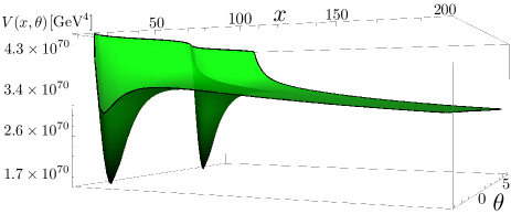
Figure 1: Potential for $r_{m}=1.0$

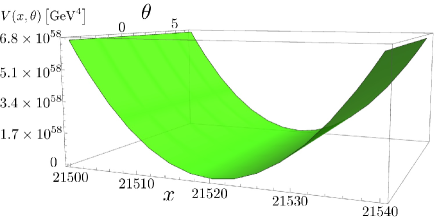
Figure 2: Potential for $r_{m}=0.1$

As seen from these figures, the values of both $V$ and $x(\theta)$ satisfying $\partial V/\partial x=0$ change rapidly depending on $\theta$ for $r_{m}=1.0$ and the values of $V$ and $x(\theta)$ are almost independent of $\theta$ for $r_{m}=0.1$.

3.2 Gauge-Higgs dominated inflation

We investigate whether the gauge-Higgs dominated inflation (an extension of the extranatural inflation) is realized based on $V(x,\theta)$. We study a case with $c_{1}=4$, $c_{2}=1$ and $r_{m}=0.3$. The reason why we choose $r_{m}=0.3$ is that the magnitude of $L^{-1}_{\rm phys}$, $m_{\rm phys}$ and $\mu_{\rm phys}$ can be larger than the reduced Planck mass if $r_{m}$ is smaller than $0.3$. Although the leading term ($k=1$) in $V(x,\theta)$ is known to be a good approximation to $V$ itself, we carry out the numerical analysis including the next-to-leading term ($k=2$) because it contributes dominantly to the second derivative of the potential with respect to $\varphi$ (the slow-roll parameter $\eta$) around $\theta=\pi/2$ .

The minimum of the potential is given by the conditions,

$$\left.V(x,\theta)\right|_{x=\langle x\rangle,\theta=\pi}=0~{},~{}~{}\left.\frac{\partial}{\partial x}V(x,\theta)\right|_{x=\langle x\rangle,\theta=\pi}=0~{},$$ (3.10)

where we use the fact that $\theta$ is fixed as $\theta=\pi$ from $\partial V/\partial\theta=0$. From (3.10), $a$ and $\langle x\rangle$ are determined as $a\simeq 2.2\times 10^{-6}m^{5}$ and $\langle x\rangle\simeq 788$. As an illustration, the $V(x,\theta)$ is depicted in Fig.3, for a specific value of $L$ and $m$.

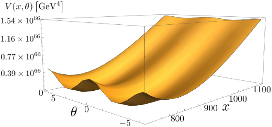
Figure 3: The potential $V(x,\theta)$ for $L=6\times 10^{-20}{\rm GeV^{-1}}$ and $m=5.1\times 10^{18}{\rm GeV}$.

From the conditions (2.3) – (2.6), we obtain the allowed region of $f$ as

$$9M_{G}\lesssim f\lesssim 15M_{G}~{}.$$ (3.11)

Hereafter, we use $f=10M_{G}$ as a typical value. Then, the initial value of $\theta$ is determined as $\theta_{\ast}=1.7$ from (2.4), and the value at the end of slow-roll is fixed as $\theta_{e}=3.0$ with $N\simeq 58$, using $\epsilon\sim 1$ and $\eta\sim 1$. In terms of $\varphi$, we have $\varphi_{\ast}=4.1\times 10^{19}{\rm GeV}$ and $\varphi_{e}=7.2\times 10^{19}{\rm GeV}$ from $\varphi=f\theta$.

The inflaton mass $M_{\varphi}$ is given by

$$M_{\varphi}^{2}=\left.\frac{\partial^{2}V}{\partial\varphi^{2}}\right|_{x=\langle x\rangle,\varphi=\langle\varphi\rangle}$$ (3.12)

and its magnitude is estimated as

$$M_{\varphi}=\left(3.2\times 10^{-48}L^{2}m^{6}{\rm GeV^{2}}\right)^{1/2}~{},$$ (3.13)

where we use (3.1) with $c_{2}=1$, $\langle x\rangle\simeq 788$, $\langle\varphi\rangle\simeq 7.2\times 10^{19}{\rm GeV}$ ($\langle\theta\rangle\simeq 3.0$) and $f=10M_{G}$. From (2.6), $L^{2}m^{6}$ is estimated as

$$L^{2}m^{6}\simeq 6.6\times 10^{73}{\rm GeV^{4}}~{}.$$ (3.14)

Using (3.13) and (3.14), the value of $M_{\varphi}$ is fixed as $M_{\varphi}\simeq 1.5\times 10^{13}{\rm GeV}$. Furthermore, we can estimate the VEV of $\chi$, using the relation $x=L^{3}m^{3}\chi$ and $\langle x\rangle\simeq 788$, as

$$\langle\chi\rangle\simeq 788L^{-3}m^{-3}~{}.$$ (3.15)

From (3.14) and (3.15), the physical mass of $U(1)$ charged fermions is determined as $m_{\rm phys}=m\langle\chi\rangle^{-1/6}\simeq 9.3\times 10^{17}{\rm GeV}$. As a reference, we estimate the masses of other particles. The radion mass $M_{\chi^{\prime}}$ is given by

$$M_{\chi^{\prime}}^{2}=\left.\frac{\partial^{2}V}{\partial\chi^{\prime 2}}\right|_{x=\langle x\rangle,\varphi=\langle\varphi\rangle}$$ (3.16)

and its value is fixed as $M_{\chi^{\prime}}\simeq 6.7\times 10^{15}{\rm GeV}$. The masses of Kaluza-Klein (KK) modes are roughly given by

$$m^{2}_{\rm KK}\sim\frac{4\pi^{2}n^{2}}{\langle\chi\rangle L^{2}}=\frac{4\pi^{2}n^{2}}{\langle\chi\rangle^{1/3}L_{\rm phys}^{2}}~{},$$ (3.17)

where $n$ is a positive integer. The mass of the first KK mode ($n=1$) is evaluated as $m_{\rm KK}|_{n=1}\simeq 6.4\times 10^{17}{\rm GeV}$.

Next, we impose the following conditions on parameters in order to limit the range of $L$.

1. The value of 4D gauge coupling constant $g_{4}$ is less than unity, in order to make the analysis based on perturbation trustworthy.

2. The physical fermion masses $m_{\rm phys}$ and $\mu_{\rm phys}$ are smaller than the 5D reduced Planck mass $M_{G_{5}}$ defined by

   $$M_{G_{5}}\equiv\sqrt[3]{\frac{1}{8\pi G_{5}}}=\sqrt[3]{\frac{1}{8\pi LG}}~{},$$ (3.18)

   where $G_{5}$ is the 5D Newton constant. From the perspective of 5D theory, $M_{G_{5}}$ would be more fundamental than the 4D one.

From i) and ii), we obtain the upper and lower bounds on $L$,

$$4.2\times 10^{-20}{\rm GeV^{-1}}\lesssim L\lesssim 6\times 10^{-18}{\rm GeV^{-1}}~{},$$ (3.19)

where we use $f=1/(g_{4}L)=10M_{G}$ and $m_{\rm phys}\simeq 9.3\times 10^{17}{\rm GeV}$. From, (3.14), (3.15) and (3.19), we have the upper and lower bounds on $m$ and $\langle\chi\rangle$,

$$1.1\times 10^{18}{\rm GeV}\lesssim m \lesssim 5.8\times 10^{18}{\rm GeV}~{},$$ (3.20)

$$2.7\lesssim \langle\chi\rangle \lesssim 55000~{}.$$ (3.21)

Note that one of $L$, $m$ and $\langle\chi\rangle$ is a free parameter. The values of physical parameters are summarized in Table 1.

Values of physical parameters
$L_{\rm phys}^{-1}=1.2\times 10^{17}\sim 6.2\times 10^{17}{\rm GeV}$
$m_{\rm phys}\simeq 9.3\times 10^{17}{\rm GeV}$
$\langle\chi^{\prime}\rangle=9.7\times 10^{17}\sim 1.1\times 10^{19}{\rm GeV}$
$\mu_{\rm phys}\simeq 2.8\times 10^{17}{\rm GeV}$
$M_{\varphi}\simeq 1.5\times 10^{13}{\rm GeV}$
$M_{\chi^{\prime}}\simeq 6.7\times 10^{15}{\rm GeV}$
$g_{4}=0.007\sim 0.9$
$M_{G_{5}}=9.9\times 10^{17}\sim 4.9\times 10^{18}{\rm GeV}$
$r\simeq 0.10$

Table 1: The allowed values of physical parameters for $f=10M_{G}$ and $r_{m}=\mu/m=0.3~{}$.

We see that $L^{-1}_{\rm phys}$, $m_{\rm phys}$ and $\mu_{\rm phys}$ are obtained as sub-Planckian quantities depending on the value of radion, even if the original parameters $L^{-1}$, $m$, $\mu$ are trans-Planckian. The $g_{4}$ can be as large as $0.9$ even if $f$ is considerably larger than $M_{G}$. It is in contrast to the result in the original extranatural inflation, i.e., $g_{4}$ turns out to be tiny of $O(10^{-2})$ [4]. The reason why $g_{4}$ can be unity in our model is that $\langle\chi\rangle$ can be much larger than $O(1)$, as seen from the relation

$$g_{4}=\frac{1}{fL}=\frac{\langle\chi\rangle^{1/3}}{fL_{\rm phys}}~{}.$$ (3.22)

The tensor-to-scalar ratio (2.7) is evaluated as $r\simeq 0.10$. It is within the range of observational upper bound, $r<0.12$ [3], but still large enough to be testable by the future observation.

From the above analysis, it is confirmed that the gauge-Higgs has properties required for the inflaton and the gauge-Higgs dominated inflation can be achieved not so unnaturally.

4 Conclusion and discussion

Using the radion gauge-Higgs potential obtained from one-loop corrections in the 5D gravity theory coupled to a $U(1)$ gauge boson and matter fermions, we have found that the gauge-Higgs $\varphi$ can give rise to a large-field inflation in accord with the astrophysical data. In contrast, it is difficult to realize the inflation dominated by the radion $\chi^{\prime}$, because the slow-roll conditions cannot be fulfilled except for a narrow region satisfying $\partial V/\partial\chi^{\prime}\simeq 0$. Furthermore, the hybrid inflation scenario is not achieved in our model that $\chi^{\prime}$ is moving toward the minimum of the potential in the first stage.

Based on the gauge-Higgs dominated inflation scenario, we have determined the values of parameters using constraints on the inflaton potential. Some of them are different from those in specific gauge-Higgs inflation models [4, 5], and this is mainly due to the difference of setup. Our model contains the gravity and the physical parameters such as the 4D gauge coupling constant $g_{4}$, the size of extra space $L_{\rm phys}$, fermion masses $m_{\rm phys}$ and $\mu_{\rm phys}$ are multiplied by some power of $\langle\chi\rangle$. Even if the parameter $f$ is trans-Planckian, i.e., $f>M_{G}$, $g_{4}$ can be as large as the standard model gauge coupling constants at the grand unified scale. This is due to the fact that $g_{4}$ is proportional to $\langle\chi\rangle^{1/3}$ and $\chi$ can take a pretty large VEV. In this case, the size of $L_{\rm phys}^{-1}$, $m_{\rm phys}$ and $\mu_{\rm phys}$ can be below the 5D reduced Planck mass. As seen from the fact that $\varphi$ works as the inflaton, $\varphi$ acquires the mass of $O(10^{13})$GeV through radiative corrections. Other massive particles are much heavier than $\varphi$. The masses of the first KK modes and the fermion zero modes are of $O(10^{17})$GeV and the radion mass is of $O(10^{15})$GeV. Because the value of radion stays almost constant in the region with $\partial V/\partial\chi^{\prime}\simeq 0$, the physical size of extra dimension has been almost stabilized at the initial time of inflation and $V(\langle\chi^{\prime}\rangle,\varphi)$ is treated as the inflaton potential effectively.

Our model is left problems concerning parameters. The first one is a common problem in inflation models, how the inflaton can take a suitable initial value to realize the inflation compatible with the observation. Because our potential has $\chi^{\prime}$ and $\varphi$, it can be traded for the initial-value-problem of $\chi^{\prime}$ that is our future work. The second one is to determine the value of $f$ without using constraints on the inflation potential. It is necessary to fix $g_{4}$ and $\langle\chi\rangle$. The value of $g_{4}$ can be obtained by the VEV of some scalar field such as the dilaton and/or the moduli. It would be efficient to extend our system by incorporating such scalar fields. The magnitude of $\langle\chi\rangle$ strongly depends on the ratio of fermion masses $r_{m}=\mu/m$. For the smaller $r_{m}$, the larger $\langle\chi\rangle$ is obtained. It would be important to explore the origin of massive fermions. The last one is how our results are reliable after receiving gravitational corrections, which are uncontrollable at present.

Furthermore, the effective field theory at the Planck scale has not yet been known. In our model, the values of several parameters can be of the order of the Planck mass and the field value of the gauge-Higgs is above the Planck scale. This result could indicate that the quantum theory of gravity such as string theory is necessary to understand the mechanism of inflation more properly. Using it, there is a possibility that gravitational corrections are controlled and our analyses are justified. In string theory construction of inflation models, the type of axion inflation is extensively studied (e.g., see [13]) for large-field inflation. We note that our effective potential is generated through the perturbative loop corrections and the origin of inflaton(s) is different from that in axion inflation models, though some of the properties of the inflaton potential, especially the periodicity, are shared. It would be interesting to study the inflation based on the effective potential relating several scalar fields such as the dilaton, the moduli (including the radion) and the gauge-Higgs in the framework of string theory.

References

- [1] D. H. Lyth and A. Riotto, Phys. Rept. 314, 1 (1999), and references therein.
- [2] For the Higgs inflation, Y. Hamada, H. Kawai and K. Oda, arXiv:1501.04455 [hep-ph], and references therein.
- [3] P. Ade et al. [Planck Collaboration], arXiv:1502.02114 [astro-ph.CO].
- [4] N. Arkani-Hamed, H.-C. Cheng, P. Creminelli, and L. Randall, Phys. Rev. Lett. 90, 221302 (2003).
- [5] T. Inami, Y. Koyama, C. S. Lim and S. Minakami, Prog. Theor. Phys. 122, 543 (2009).
- [6] Y. Fukazawa, T. Inami, and Y. Koyama, Prog. Theor. Exp. Phys. 2013 021B01 (2013).
- [7] Y. Hosotani, Phys. Lett. B126, 309 (1983).
- [8] Y. Abe, T. Inami, Y. Kawamura and Y. Koyama, Prog. Theor. Exp. Phys. 2014 073B04 (2014).
- [9] T. Appelquist and A. Chodos, Phys. Rev. D 28, 772 (1983).
- [10] E. Ponton and E. Poppitz, JHEP 0106, 019 (2001).
- [11] A. D. Linde, Phys. Rev. D 49, 748 (1994).
- [12] K. Kohri, C.S. Lim, and C.M. Lin, JCAP 1408, 001 (2014).
- [13] L. McAllister, E. Silverstein, A. Westphal and T. Wrase, JHEP 1409, 123 (2014)