The Social Cost of Carbon with
Economic and Climate Risks

Abstract

There is great uncertainty about future climate conditions and the appropriate policies for managing interactions between the climate and the economy. We develop a multidimensional computational model to examine how uncertainties and risks in the economic and climate systems affect the social cost of carbon (SCC)—that is, the present value of the marginal damage to economic output caused by carbon emissions. The SCC is substantially increased by economic and climate risks at both current and future times. Furthermore, the SCC is itself a stochastic process with significant variation; for example, the basic elements of risk incorporated into our model cause the SCC in 2100 to be, with significant probability, ten times what it would be without those risks. We have only imprecise information about what parameter values are best for approximating reality. To deal with this parametric uncertainty we perform extensive uncertainty quantification and show that these findings are robust for a wide range of alternative specifications. More generally, this work shows that large-scale computing can enable economists to examine substantially more complex and realistic models for the purposes of policy analysis.

Key words: Climate policy, social cost of carbon, climate tipping process, Epstein–Zin preferences, stochastic growth, long-run risk

1 Introduction

Global warming has been recognized as a growing potential threat to economic well-being. This concern has lead to an increasing number of national and international discussions on how to respond to this threat. Determining which policies should be implemented will require merging quantitative assessments of the likely economic impacts of carbon emissions with models of how the economic and climate systems interact; this is the purpose of integrated assessment models (IAMs). This paper expands the scope of IAMs by adding uncertainties and risks to a canonical model of the economic and climate systems, and shows that such risks significantly raise the optimal level of carbon emission mitigation.

The impact of carbon emissions on society is measured by the social cost of carbon (SCC), defined as the marginal economic loss caused by an extra metric ton of atmospheric carbon. The Intergovernmental Panel on Climate Change (IPCC), whose reviews summarize scientific studies on climate change, reports that estimates of the SCC vary across studies with an average estimate of $43 per ton of carbon (Yohe et al. 2007). The Interagency Working Group on Social Cost of Carbon (IWG)—a joint effort involving several United States federal agencies—came to similar conclusions in a report based on often-used integrated assessment models (IWG 2010). Most IAM models assume myopic expectations. The DICE (Dynamic Integrated Climate and Economy) model of Nordhaus (2008) is one of the few forward-looking integrated assessment models and suggests a social cost of carbon of $35 per ton of carbon. This rough consensus has been challenged by Pindyck (2013) and IPCC (2014), who argue that all of these estimates are limited because they come from IAMs that ignore the considerable risk and uncertainty in both the economic and the climate system, and their interactions. Those models also assume that people are far less risk averse than indicated by economic observations of the price of risk.

This study presents Dynamic Stochastic Integration of Climate and the Economy (DSICE), a computational, dynamic, stochastic general equilibrium framework for studying global models of both the economy and the climate. We apply it to the specific issue of how the social cost of carbon depends on stochastic features of both the climate and the economy when we apply empirically plausible specifications for the willingness to pay to reduce economic risk. The examples we study demonstrate the flexibility of the DSICE framework.

We first examine how economic risks affect the social cost of carbon. Specifically, we assume that factor productivity growth displays long-run risk as modeled by Bansal and Yaron (2004) and Beeler and Campbell (2011). We calibrate the stochastic productivity growth process to match observed moments of the growth rates for per capita consumption. We combine this with recursive utility specifications of dynamic preferences that use parameter values consistent with observations about how much people are willing to pay to reduce consumption risk. This version of our model demonstrates that realistic specifications of risks in the economic system will imply substantially greater social costs of carbon; for example, the 2005 SCC in our benchmark parameter case is $61 per ton of carbon, 65 percent larger than the SCC in the absence of productivity shocks.

Current empirical analyses do not give us precise estimates of critical parameters. Therefore, following the response surface methods from the uncertainty quantification literature (see Oberkampf and Roy (2010) for a comprehensive discussion of verification, validation, and uncertainty quantification (VVUQ)), we also examine a large set of empirically plausible values for key parameters, such as the risk aversion parameter and the elasticity of inter-temporal substitution. We find that the 2005 SCC ranges from $35 to $115 per ton of carbon over the parameter values we consider. These results demonstrate that we should be skeptical of studies that rely on a single parameterization, but the application of uncertainty quantification methods supports the qualitative claim that economic risks significantly increase the SCC.

Of equal interest and greater novelty are our results on the dynamics of the future SCC. Stochastic factor productivity creates riskiness in future output and carbon emissions, which in turn makes the SCC a random process. Conventional IAMs assume no riskiness and produce a deterministic path for the future SCC. A common interpretation of results in deterministic models is that a quantity’s path represents its expectation in more realistic models. In many cases, we find that the mean path for the SCC is close to that implied by deterministic models, thereby confirming the value of deterministic models for approximating expectations. DSICE, however, can also determine the stochastic features of the SCC process and shows that the SCC is approximately a random walk with substantial variance. For example, in our benchmark case the expected SCC is $286 in 2100 but with a 10% chance of exceeding $700 and a 1% chance of exceeding $1,200. In general, the variance of the social cost of carbon grows faster than its mean. Any description of the future must recognize both the intrinsic risk in any fixed model and our uncertainty about the best values for parameters. Combining parameter uncertainty with intrinsic risk implies a substantially larger range for the future SCC.

The second source of uncertainty incorporated into DSICE is uncertainty about how the climate will respond to anthropogenic emissions. Most integrated assessment models assume that the impact of climate on productivity depends only on the contemporaneous temperature. This implies a smooth, predictable and reversible pattern of damages from global warming. The stochastic climate feature we add is based on the recent literature on climate tipping elements. These are defined as any subsystem of the Earth’s system that could exhibit critical points (tipping points) where the climate abruptly and unexpectedly jumps to a qualitatively different state (Lenton et al. 2008). The climate literature has identified several major tipping elements in the climate system. Recent projections suggest that the irreversible melting of the Greenland ice sheet could be triggered during this century (IPCC 2014); such melting could cause the global sea level to rise by 0.5–1.0 meter per century (Lenton et al. 2008). Joughin et al. (2014) argue that the collapse of the west Antarctic ice sheet is already under way. Other examples of climate tipping elements include the weakening or shutdown of the Atlantic thermohaline circulation and the dieback of the Amazon rainforest. Current temperature affects the likelihood of crossing a tipping point, but temperature reversals will not reverse the tipping event.

Tipping points bring a new dimension to the modeling of the climate’s effect on the economy. For example, once warming melts a glacier, that glacier will not reform even if the warming is reversed, and damages arising from the rising sea levels will persist. Tipping phenomena bring a qualitative new feature to climate damage in that some of the current damage to productivity is due to past warming. A recent review recommends that we should seriously consider climate tipping points in order to better anticipate and prepare ourselves for the inevitable, potentially adverse surprises they bring (National Research Council 2013).

DSICE is sufficiently flexible to incorporate tipping elements of various kinds in terms of probability, duration, and impact levels. This allows us to consider a range of beliefs about the likelihood of warming triggering a climate tipping point, and to determine how optimal policy and the social cost of carbon depend on the characteristics of a tipping element. For our benchmark parameter specification of preferences, stochastic growth, and the climate tipping process we find that the 2005 social cost of carbon is $125 per ton of carbon, but a value of $354 is also consistent with plausible specifications for climate tipping processes.

Some studies (e.g., Weitzman 2009) use the possibility of very high damage caused by a very low probability catastrophic event to advocate aggressive mitigation policies. Estimating the probability of tail events is very difficult, a fact that reduces the force of these arguments. Our DSICE results show that climate tipping specifications that imply bad, but not catastrophic, events can imply a very high social cost of carbon. Extreme disaster scenarios are not the only assumptions that justify high social costs of carbon.

Uncertainty about damage from a climate tipping event raises the social cost of carbon in a manner similar to the impact of risk in consumption-based capital asset pricing models: the social cost of carbon is proportional to the variance of uncertainty regarding damage. One interpretation of such variance is that it represents our ignorance of damage from the climate tipping process. This observation shows that DSICE could be used to determine which scientific studies would be most cost-effective in reducing the uncertainties faced by policymakers. This is just one example of how the DSICE framework could be applied in future studies.

Our models demonstrate that any discussion of the social cost of carbon must consider stochastic elements in both the climate and the economic system. We also find that these elements have nontrivial interactions. For example, in our default parameter cases each component—when studied in isolation—sharply elevates the social cost of carbon, but when both economic and climate risks are included the resulting SCC process lies in between the levels of the individual effects. One cannot just look at these risks in isolation and advance some ad hoc argument on how to aggregate results across studies.

The ability of DSICE to track the stochastic behavior of the social cost of carbon makes it a potential tool for assessing a variety of policy questions because uncertainties about the social cost of carbon will affect the ranking of alternative policies. R&D decisions are certainly one example of this. R&D decisions made today will determine the mitigation methods available in future decades. A deterministic model would compare the expected benefits with the expected costs, using the discount rate that is applied to all inter-temporal decisions. This procedure is not valid in a dynamic stochastic context. For instance, our results show that there is a good chance that the social cost of carbon will be so high in a few decades that optimal policy would not only reduce carbon emissions but would also use technologies that remove carbon from the atmosphere. The development of such technologies could take decades to complete. Policy discussions today about R&D investment in developing those technologies should not compare the expected social cost of carbon in the future with the expected results of R&D investments, but should focus instead on the present value of having such technologies in those states of the world where the SCC justifies their deployment.

The R&D illustration is just one example of a more general and important point. In deterministic models, mitigation spending is a form of investment and subjected to the same net present value criterion as all other investments. There is a consensus that the choice of discount rate is a major determinant of optimal policy (e.g., Stern 2007 and Nordhaus 2007). Some have argued that this is not the right way to think about mitigation expenditures in an uncertain and risky world. Schneider (1989), in his testimony to the Committee on Energy and Commerce in 1989, argued that investing in climate change mitigation is like "buying insurance against the real possibility of large and potentially catastrophic climate change." DSICE is the first IAM modeling framework that can capture insurance and hedging values of climate change policies. Further development of these ideas must be left to future research, but basic economic intuition suggests that real option values and insurance ideas will play significant roles in evaluating alternative policies.

This study also demonstrates the value of modern high-power computing in studying basic economics questions. The versions of DSICE that we examine are stochastic, nine-dimensional, nonlinear dynamic programming problems. Including stochastic productivity requires the use of annual time periods, and the long-run nature of climate change requires a multi-century time span. The non-stationary character of the problems makes value function iteration the only appropriate approach. The specifications of risks make these problems among the most computationally demanding ever solved in economics. We are able to solve them because we use efficient multivariate methods to approximate value functions, and reliable optimization methods to solve the Bellman equations (Cai and Judd 2010; Cai et al. 2015). Any numerical computation has numerical errors. Another theme of the VVUQ literature is that computational results should be tested to verify their accuracy. Every value function we compute passes demanding verification tests, giving us confidence that numerical errors do not affect our economic conclusions. Some examples required tens of thousands of core hours, and sensitivity analysis demanded that we examine hundreds of cases to determine the robustness of results across empirically plausible parameter values. This study required the use of a few million core hours on Blue Waters, a modern supercomputer. Our use of general purpose methods shows that many economics problems with similar computational requirements can now be solved.

The structure of this paper is as follows. Section 2 compares our work with other studies. We present the economic model in Section 3 and the climate model in Section 4. In Section 5 we formulate the dynamic programming problem, outline its solution method, and present a general calibration strategy. Sections 6, 7, and 8 present and discuss implications for the social cost of carbon from stochastic specifications of factor productivity growth and a climate tipping process; first each in isolation and then combined. Section 9 concludes.

2 Relation to the Literature

Our work contributes to the popular debate on how urgently policymakers should address climate change issues. Many cost-benefit analyses of climate change, such as that of Nordhaus (2008), suggest global climate policy should be relatively weak. Others, including Pindyck (2013), Kopits et al. (2014), Lenton and Ciscar (2013), and Ackerman et al. (2013) have criticized these analyses for their unrealistic specifications. In DSICE, we describe the uncertainty regarding economic growth and future climate impacts in more realistic ways and support recent suggestions, such as those made in Revesz et al. (2014), that the costs of carbon emissions are underestimated.

DSICE follows recent developments in macroeconomic theory and data analysis. Macroeconomists have recently argued that economic output follows processes with persistence in growth rates, and that recursive preferences do the best in terms of representing attitudes towards risk. These insights have been included in a few recent papers on global warming using simplified models. Bansal and Ochoa (2011) assume that consumption and output are exogenous stochastic processes. DSICE instead builds on a Ramsey-type, representative agent, stochastic growth model. We calibrate the stochastic factor productivity growth so that the resulting consumption process is statistically close to empirical data. Jensen and Traeger (2014) includes endogenous output but assumes much lower volatility than implied by empirical data. Moreover, Jensen and Traeger (2014) assume that carbon emissions have an immediate impact on economic productivity, whereas DSICE and most integrated assessment models assume a time lag between emissions and impacts. Ignoring this lag will likely overestimate the SCC and will create an unrealistically strong correlation between short-run fluctuations in atmospheric carbon and their economic impacts.

DSICE also adds tipping events to the standard IAM model form. The climate literature has identified several major tipping elements in the climate system. An example of a major tipping element is irreversible melting of the Greenland ice sheet. Recent projections of future global warming suggest that it is more likely than not that the Greenland ice sheet tipping point will be triggered within this century (IPCC 2014). Joughin et al. (2014) argue that marine west Antarctic ice sheet collapse is already under way. Melting of the Greenland ice sheet (which contains the equivalent of about seven meters of global sea level) could lead to a global sea level rise of up to 0.5–1 meter per century (Lenton et al. 2008). Other examples of climate tipping elements include the weakening or shutdown of the Atlantic thermohaline circulation or the dieback of the Amazon rainforest.

Economic analyses of tipping elements have used a variety of specifications, ranging from purely deterministic representations (e.g., Keller et al. 2004; Mastrandrea and Schneider 2001; Nordhaus 2012; and Weitzman 2012) to fully stochastic specifications (e.g., Polasky et al. 2011; Brock and Starrett 2003; and Lemoine and Traeger 2014). However, stochastic formulations of tipping processes have not been incorporated into major integrated assessment models such as that of Nordhaus (2008). Our computational method can deal with this complexity.

Our tipping element specification is also the first to address the recent critique by Kopits et al. (2014) of current studies which assume that the full impact of a climate tipping point is immediate and its level is known (see, e.g., Lemoine and Traeger 2014). The nature of climate tipping point events is very different from that currently being assumed in economic models. The occurrence, or not, of the tipping point is unknown, the transition time of the tipping process is unknown, and—furthermore—the impact of the climate tipping is unknown (Lenton et al. 2008; National Research Council 2013).

The structure of DSICE and its calibration strategy enable us to retain the deterministic integrated assessment model in Nordhaus’s (2008) model as a special case of DSICE, when we eliminate all shocks to climate and the economy and adjust the preference parameters accordingly. The model in Nordhaus (2008) is currently being used by the United States government to design climate policy (IWG 2010) and we wish to compare its implications for climate policy with those obtained from our modeling approach. However, we will note that DSICE is not just a stochastic extension of earlier versions of Nordhaus (2008). Our framework can be used to solve many integrated assessment models of comparable dimensionality.

The distinctive feature of DSICE is that it combines stochastic factor productivity growth with uncertainty about adverse, irreversible climate events, uses recursive preferences, and enables us to examine and quantify the impact of economic and climate risks on the social cost of carbon. No computational framework is infinitely powerful, but it is clear that DSICE is far less limited by tractability concerns than are earlier integrated assessment models. Future work will take advantage of our framework and computational strengths to study alternative models, even ones larger than those examined below.

3 The Economic Model

Our model’s framework merges a basic dynamic stochastic general equilibrium model with a commonly used climate model. The canonical “Dynamic Integrated Climate–Economy” (DICE) model (Nordhaus, 2008) will be a special case of our dynamic stochastic integrated assessment framework. In particular, DSICE includes two stochastic processes not part of earlier integrated assessment models.

First, we include an exogenous stochastic process that affects productivity. This productivity process could represent an autoregressive productivity shock, or a process that implies consumption processes similar to those described in the literature on stochastic growth with persistence.

Second, we include a finite-state Markov process, $J_{t}$, that also affects productivity but with transitions that are affected by temperature, making $J_{t}$ an endogenous process representing the impact of past climate change on current productivity. In this paper, $J_{t}$ models tipping elements in climate dynamics (Kriegler et al. 2009 and Lenton et al. 2008), a feature of climate change dynamics that has only recently has been studied by climate scientists.

We describe the economic model in detail in this section, including only those climate elements that directly relate to productivity. A later section gives the details of the climate system. This approach to exposition helps make clear the two distinct systems, climate and economy, and their interactions. Regarding the calibration of DSICE for numerical results, we present our calibration strategy in Section 5.2 while a list of all parameters and exogenous processes of the economic model appears in Appendices A and B.

3.1 Production

The economic side of DSICE is a simple stochastic growth model where production produces greenhouse gas emissions and productivity is affected by the state of the climate. In this section we will model the climate system in a general fashion that only describes the interactions between climate and economic productivity. The next section will give the motivation for and specification of the climate module. One advantage of this approach is that it makes clear the limited nature of the linkages between climate and economy and also makes clear how one can replace our climate module with any alternative.

We assume time is discrete, with each period equal to one year. Let $K_{t}$ be the world capital stock in trillions of dollars at time $t$ and $L_{t}$ be the world population in millions at time $t$. We use the exogenous population path from Nordhaus (2008)

$$L_{t}=6514e^{-0.035t}+8600(1-e^{-0.035t})$$ (1)

In the absence of any climate damage, the gross world product is described by a Cobb–Douglas production function with

$$f(K,L,\widetilde{A}_{t})=\widetilde{A}_{t}K^{\alpha}L^{1-\alpha},$$

where $\alpha=0.3$ (as in Nordhaus, 2008) and $\widetilde{A}_{t}$ is productivity at time $t$. Productivity is decomposed into two pieces: a deterministic trend $A_{t}$, and a stochastic productivity state $\zeta_{t}$, that is to say that $\widetilde{A}_{t}\equiv\zeta_{t}A_{t}$. The deterministic trend $A_{t}$ is taken from Nordhaus (2008) and equals

$$A_{t}=A_{0}\exp\left(\alpha_{1}(1-e^{-\alpha_{2}t})/\alpha_{2}\right),$$ (2)

where $\alpha_{1}$ is the initial growth rate and $\alpha_{2}$ is the decline rate of the growth rate. We want to examine how uncertainty in productivity interacts with climate change policies.

We use one extra state $\chi_{t}$ to help model the stochastic productivity state $\zeta_{t}$, where $\chi_{t}$ represents the persistence of $\zeta_{t}$. More specifically, we start with the formulation introduced in Bansal and Yaron (2004) with the following form:

$$\log\left(\zeta_{t+1}\right)=\log\left(\zeta_{t}\right)+\chi_{t}+\varrho\omega_{\zeta,t}$$ (3)

$$\chi_{t+1}=r\chi_{t}+\varsigma\omega_{\chi,t}$$ (4)

Bansal and Yaron assumed that $\omega_{\zeta,t},\omega_{\chi,t}\sim i.i.d.\>\mathcal{N}(0,1)$ and $\varrho$, $r$, and $\varsigma$ are parameters. Gaussian disturbances are, unfortunately, unbounded and would produce arbitrarily large growth rates and output, creating an unbounded optimal growth problem where even the existence of expected utility is unclear. Even if we could overcome the theoretical and computational challenges, results for the social cost of carbon could be driven by highly unlikely tail events. An example of this is the dismal theorem of Weitzman (2009) showing that the risk premium could be infinite for unboundedly distributed uncertainties. We do want to avoid existence issues and excessive dependence on extreme tail events. To this end, we construct a time-dependent, finite-state Markov chain for $\left(\zeta_{t},\chi_{t}\right)$ that implies conditional and unconditional moments of consumption processes calibrated to observed market data. The Markov transition processes are denoted $\zeta_{t+1}=g_{\zeta}(\zeta_{t},\chi_{t},\omega_{\zeta,t})$ and $\chi_{t+1}=g_{\chi}(\chi_{t},\omega_{\chi,t})$, where $\omega_{\zeta,t}$ and $\omega_{\chi,t}$ are two serially independent stochastic processes. This approach also makes it possible to directly apply reliable numerical methods for solving dynamic programming problems. Appendix B describes these features in greater detail.

DSICE assumes that output is affected by temperature. The production function $f\left(K_{t},L_{t},\widetilde{A}_{t}\right)$ represents output in the absence of any effects of climate on output.

The impact of climate on output in DSICE will depend on two climate states : global average temperature $T_{\mathrm{AT}}$, and a climate state denoted by $J$. The climate state $J$ will model cumulative effects of past temperatures and is represented by a finite-state Markov chain In this paper, we parameterize $J$ to represent stages in a climate tipping processes; therefore, we will refer to it as the “tipping state.” DSICE also contains other climate states but this version assumes that only the states $T_{\mathrm{AT},t}$ and $J_{t}$ directly affect economic decisions..

The function $\Omega\left(T_{\mathrm{AT},t},J_{t}\right)$ represents the impact of climate on output, and gross world product equals

$$\mathcal{Y}_{t}\left(K_{t},T_{\mathrm{AT},t},\zeta_{t},J_{t}\right)=\Omega\left(T_{\mathrm{AT},t},J_{t}\right)f\left(K_{t},L_{t},\zeta_{t}A_{t}\right),$$

where

$$\Omega\left(T_{\mathrm{AT},t},J_{t}\right)=\frac{1-J_{t}}{1+\pi_{1}T_{\mathrm{AT},t}+\pi_{2}(T_{\mathrm{AT},t})^{2}}.$$

As is common in the IAM literature, we will call $\Omega\left(T_{\mathrm{AT},t},J_{t}\right)$ the damage function. We will examine only cases where $\Omega\left(T_{\mathrm{AT},t},J_{t}\right)$ is bounded by unity, but that is not a requirement in our general framework. When $J_{t}=0$, a state we will call the “pre-tipping state”, our damage function reduces to the damage function in Nordhaus (2008), which is widely used in the literature. This study generalizes the damage function to include effects of the “tipping state” and associated past cumulative effects. The definition of $J$ implies $0\leq J_{t}\leq 1$; therefore, the numerical value of the tipping state $J_{t}$ equals the current damage caused by past tipping events, so we also call $J_{t}$ the “tipping damage level” when $J_{t}>0$. The stochastic dynamic structure of $J_{t}$ is specified in more detail below in the section on the climate model.

The economic system affects the climate through emissions of carbon. We assume that industrial emissions are proportional to output, with proportionality factor $\sigma_{t}$ representing the carbon intensity of output. The social planner can mitigate (i.e., reduce) emissions by a factor $\mu_{t}$ with $0\leq\mu_{t}\leq 1$. The annual industrial carbon emissions (billions of metric tons of carbon) equal

$$E_{\mathrm{Ind},t}\left(K_{t},\mu_{t},\zeta_{t}\right)=\sigma_{t}(1-\mu_{t})f\left(K_{t},L_{t},\zeta_{t}A_{t}\right).$$ (5)

We follow Nordhaus (2008) and assume that mitigation expenditures equal

$$\Psi_{t}=\theta_{1,t}\mu_{t}^{\theta_{2}}\mathcal{Y}_{t}\left(K_{t},T_{\mathrm{AT},t},\zeta_{t},J_{t}\right).$$ (6)

World output (net of damage) is allocated across total consumption $C_{t}$, mitigation expenditures $\Psi_{t}$, and gross capital investment $I_{t}$, that is to say

$$\mathcal{Y}_{t}=C_{t}+\Psi_{t}+I_{t},$$ (7)

thus the capital stock evolves according to

$$K_{t+1}=(1-\delta)K_{t}+I_{t}$$ (8)

where $\delta=0.1$ is the annual depreciation rate.

3.2 Epstein–Zin Preferences

The additively separable utility functions commonly used in climate-economy models do not do well in explaining the willingness of people to pay to avoid risk. Here instead, we use Epstein–Zin preferences (Epstein and Zin 1989). Let $C_{t}$ be the stochastic consumption process. Epstein–Zin preferences recursively define the social welfare as

$$U_{t}=\left\{\left(1-\beta\right)u(C_{t},L_{t})+\beta\left[\mathbb{E}_{t}\left\{U_{t+1}^{1-\gamma}\right\}\right]^{\frac{1-1/\psi}{1-\gamma}}\right\}^{\frac{1}{1-1/\psi}},$$ (9)

where $\mathbb{E}_{t}\mathbb{\left\{\cdot\right\}}$ is the expectation conditional on the states at time $t$, and $\beta$ is the discount factor. Here,

$$u(C_{t},L_{t})=\frac{\left(C_{t}/L_{t}\right)^{1-1/\psi}}{1-1/\psi}L_{t}$$

is the annual world utility function (assuming that each individual has the same power utility function), $\psi$ is the inter-temporal elasticity of substitution, and $\gamma$ is the risk aversion parameter. Epstein–Zin preferences are flexible specifications of decision-makers’ preferences regarding uncertainty, and allow us to distinguish between risk preference and the desire for consumption smoothing. Even though we refer to $\gamma$ as the risk aversion parameter, the equilibrium risk premia will depend on interactions between $\psi$ and $\gamma$. Epstein–Zin preferences are special cases of Kreps–Porteus preferences (Kreps and Porteus 1978), which were designed to model preferences over the resolution of risk. For the special case where $\psi\gamma=1$, we have the separable utility case used in Nordhaus (2008).

Epstein–Zin preferences are used here because they better explain observed equity premia. Even though climate change risks are not directly related to equity returns, observations about the equity premia inform us about society’s willingness to pay to reduce consumption risk. Therefore, we expect the optimal climate policy to be affected by uncertainty regarding the economic damage arising from climate change.

4 The Climate Model

Our climate model contains three modules. The first module is the carbon system and the second is the temperature module, both of which are deterministic and adapted from the integrated assessment model of Nordhaus (2008). The underlying idea is that industrial emissions of greenhouse gases increase atmospheric carbon concentrations, causing an increase in global average temperature, which then reduces economic productivity as specified above.

We also add a stochastic tipping element module which represents a state of the climate related to past climate conditions and events. A simple example of such a climate state is sea level. Prolonged periods of warm atmospheric temperatures will (likely) melt ice in glaciers (on land) which will then lead to a higher sea level, which can be viewed as a state variable that affects economic productivity due to, for example, flooding. The addition of the climate tipping module and its associated uncertainties adds a novel element to integrated assessment modeling.

We present our calibration strategy for these modules in Section 5.2 while a list of all parameters and exogenous processes of the model appears in Appendices A and D.

4.1 Carbon Module

We assume two sources for carbon emissions, an industrial source $E_{\mathrm{Ind},t}\left(K_{t},\mu_{t},\zeta_{t}\right)$ specified above and an exogenous source, $E_{\mathrm{Land},t}$, arising from land use. Total emissions are denoted

$$\mathcal{E}_{t}\left(K_{t},\mu_{t},\zeta_{t}\right)=E_{\mathrm{Ind},t}\left(K_{t},\mu_{t},\zeta_{t}\right)+E_{\mathrm{Land},t}.$$ (10)

Carbon is distributed across three “boxes” representing different carbon concentrations. The three-dimensional vector ${\bf M}_{t}=(M_{\mathrm{AT},t},M_{\mathrm{UO},t},M_{\mathrm{LO},t})^{\top}$ represents the mass of carbon concentrations in the atmosphere, and in the upper levels of the ocean and lower levels of the ocean, respectively (in gigatons of carbon). The carbon cycle specifies how these concentrations evolve over time and is represented by the linear dynamical system

$$\mathbf{M}_{t+1}=\mathbf{\Phi}_{M}\mathbf{M}_{t}+\left(\mathcal{E}_{t},0,0\right)^{\top},$$

where $\mathbf{\Phi}_{M}$ is the matrix

$$\mathbf{\Phi}_{M}=\left[\begin{array}[]{ccc}1-\phi_{12}&\phi_{21}&0\\ \phi_{12}&1-\phi_{21}-\phi_{23}&\phi_{32}\\ 0&\phi_{23}&1-\phi_{32}\end{array}\right].$$ (11)

The coefficients of the matrix $\mathbf{\Phi}_{M}$ have natural interpretations. The coefficient $\phi_{ij}$ is the rate at which carbon diffuses from level $i$ to level $j$, for $i,j\in$ {atmosphere, upper ocean, lower ocean}. Since this is a closed system except for the emission input $\mathcal{E}_{t}$, the column sums of $\mathbf{\Phi}_{M}$ must be unity.

4.2 Temperature Module

The temperature module models two temperatures in the atmosphere and the ocean, measured in degrees Celsius. That system is represented by the vector ${\bf T}_{t}=(T_{\mathrm{AT},t},T_{\mathrm{OC},t})^{\top}$, and evolves according to

$$\mathbf{T}_{t+1}=\mathbf{\Phi}_{T}^{\mathrm{}}\mathbf{T}_{t}+\left(\xi_{1}\mathcal{F}_{t}\left(M_{\mathrm{AT},t}\right),0\right)^{\top},$$ (12)

where the heat diffusion process between ocean and air is represented by the matrix

$$\mathbf{\Phi}_{T}=\left[\begin{array}[]{cc}1-\varphi_{21}-\xi_{2}&\varphi_{21}\\ \varphi_{12}&1-\varphi_{12}\end{array}\right].$$ (13)

The coefficient $\varphi_{ij}$ is the heat diffusion rate from level $i$ to level $j$, for $i,j\in$ {atmosphere, ocean}, and $\xi_{2}$ is the rate of atmospheric temperature change by infrared radiation to space (Schneider and Thompson 1981). Atmospheric temperature is affected by exogenous external forcing, $F_{\mathrm{EX},t}$, and by interactions between radiation and carbon in the atmosphere. Total radiative forcing at $t$ is

$$\mathcal{F}_{t}\left(M_{\mathrm{AT},t}\right)=\eta\log_{2}\left(M_{\mathrm{AT},t}/M_{\mathrm{AT}}^{*}\right)+F_{\mathrm{EX},t},$$ (14)

where $M_{\mathrm{AT}}^{*}$ is the preindustrial atmospheric carbon concentration and $\eta$ is the radiative forcing parameter.

4.3 Tipping Element Module

We next describe the dynamics of $J_{t}$, the climate state representing the effects of past temperatures on some aspect of the climate that is not captured by the current temperatures and carbon states. We choose a Markov chain for $J_{t}$ so that the changes in $J_{t}$ model a tipping with damage as a function of that state. At each time $t$, $J_{t}$ is one of the finite number of states in the set denoted $\left\{\mathcal{J}_{1},\mathcal{J}_{2},...,\mathcal{J}_{n_{\negthinspace J}}\right\}$ for some positive integer $n_{\negthinspace J}$. The transition probabilities depend on climate states in a general way, but this study considers tipping elements only. With this focus, we will use terminology appropriate for climate tipping elements.

At the initial time, the state of the tipping element is represented by $J_{t}=0$. A common approach is to assume that a tipping point is defined by a definite (but possibly unknown to the planner) threshold, the crossing of which leads immediately to abrupt change. We instead assume that a tipping point is a probabilistic function of climate conditions. Specifically, we follow the common assumption that warming alone causes tipping (IPCC 2014; Smith et al. 2009), but assume that if $J_{t}=0$, the probability that tipping does not occur in the year $t$ equals

$$p_{1,1,t}=\exp\left\{-\lambda\max\left\{0,\,T_{\mathrm{AT},t}-\underline{T_{\mathrm{AT}}}\right\}\right\},$$ (15)

where $\lambda$ is the (linear) hazard rate parameter and $\underline{T_{\mathrm{AT}}}$ is the temperature for which $p_{1,1,t}=1$.

One common approach to modeling tipping events is to assume a critical (but perhaps unknown) temperature threshold such that the tipping event happens if temperature reaches the threshold (see Keller et al. 2004). With economic uncertainty, temperatures can fall or rise. If temperature were to cross a threshold, the tipping event would immediately happen even if the temperature quickly fell below the threshold. We prefer a smoother representation of how climate subsystems respond to world average temperature, such as accomplished with our specification in (15).

Once tipping has occurred, there will be more transitions of $J_{t}$. This study assumes irreversibility, implying that all positive probability transitions increase $J_{t}$. Integrated assessment models that include a tipping element typically assume that all impacts are realized immediately (e.g., Lemoine and Traeger 2014). In our framework, that is equivalent to assuming there are only two climate states related to tipping: $\left\{\mathcal{J}_{1},\mathcal{J}_{2}\right\}$. However, climate scientists do not regard this as a realistic description of the tipping elements they consider. Lenton et al. (2008) characterize the transition scales for various tipping elements, arguing, for example, that the loss of Arctic summer sea-ice could be complete after about ten years, but that the melting of the Greenland ice sheet would, once it began, continue for more than three hundred years before reaching its long-run state. In DSICE we present more appropriate specifications for the Markov chain states $\left\{\mathcal{J}_{1},\mathcal{J}_{2},...,\mathcal{J}_{n_{\negthinspace J}}\right\}$ and the transition probabilities, and can examine the more realistic and general tipping elements preferred by climate scientists. The applications of DSICE presented below will examine a variety of specifications for the details of the Markov process that represents the effects of tipping elements.

5 The Dynamic Programming Problem

We formulate the nine-dimensional, social planner’s dynamic optimization problem as a dynamic programming problem. The nine states include six continuous state variables (the capital stock $K$, the three-dimensional carbon system $\mathbf{M}$, and the two-dimensional temperature vector $\mathbf{T}$) and three discrete state variables (the climate shock $J$, the stochastic productivity state $\zeta$, and the persistence of its growth rate, $\chi$). Let $\mathbf{S}\equiv\left(K,\mathbf{M},\mathbf{T},\zeta,\chi,J\right)$ denote the nine-dimensional state variable vector and let $\mathbf{S}^{+}$ denote its next period’s state vector.

The Epstein–Zin utility definition expressed utility in terms of consumption. We make a nonlinear change of variables and express the Bellman equation in terms of utils, $\left(U_{t}\right)^{1-\frac{1}{\psi}}$ . The Bellman equation then becomes

$$V_{t}\left(\mathbf{S}\right)=\max_{C,\mu} u(C_{t},L_{t})+\beta\left[\mathbb{E}_{t}\left\{\left(V_{t+1}\left(\mathbf{S}^{+}\right)\right)^{\frac{1-\gamma}{1-1/\psi}}\right\}\right]^{\frac{1-1/\psi}{1-\gamma}},$$

s.t. $$K^{+}=(1-\delta)K+\mathcal{Y}_{t}(K,T_{\mathrm{AT}},\zeta,J)-C_{t}-\Psi_{t},$$ (16)

$$\mathbf{M}^{+}=\mathbf{\Phi}_{M}\mathbf{M}+\left(\mathcal{E}_{t}\left(K,\mu,\zeta\right),0,0\right)^{\top},$$

$$\mathbf{T}^{+}=\mathbf{\Phi}_{T}\mathbf{T}+\left(\xi_{1}\mathcal{F}_{t}\left(M_{\mathrm{AT}}\right),0\right)^{\top},$$

$$\zeta^{+}=g_{\zeta}(\zeta,\chi,\omega_{\zeta}),$$

$$\chi^{+}=g_{\chi}(\chi,\omega_{\chi}),$$

$$J^{+}=g_{J}(J,\mathbf{T},\omega_{J}),$$

for $t=0,1,\ldots,599$, and any $\psi>1$. The terminal value function $V_{600}$ is given in Appendix E. In the model, consumption $C$ and emission control rate $\mu$ are two control variables.

5.1 The Social Cost of Carbon

In this paper, we follow the jargon of the climate literature which interprets the social cost of carbon as a marginal concept–that is to say, the monetized economic loss caused by an increase in atmospheric carbon by one metric ton. In our model, the social cost of carbon is the marginal cost of atmospheric carbon expressed in terms of the numeraire good, which can be either consumption or capital as there are no adjustment costs. We define the social cost of carbon (SCC) to be the marginal rate of substitution between atmospheric carbon concentration and capital, as in

$$\mathrm{SCC}_{t}=-1000\left(\partial V_{t}/\partial M_{\mathrm{AT},t}\right)/\left(\partial V_{t}/\partial K_{t}\right).$$ (17)

It will be important to remember that the social cost of carbon is a relative shadow price–that is to say, a ratio of two marginal utilities, and does not express the total social cost of climate damage. For example, as we change economic and/or climate risks, the social cost of carbon may go up or down because that change in risks will affect both the marginal value of carbon and the marginal cost of consumption (or, equivalently, the marginal value of investment). DSICE is a general equilibrium model where the results arise from the assumptions about tastes and technology as well as their equilibrium interactions.

Often, the social cost of carbon and the term carbon tax are used interchangeably. The optimal carbon tax is the tax on carbon that would equate private and social costs of carbon. In our model we also examine the optimal carbon tax, which is the Pigovian tax policy because the externality from carbon emissions can be directly dealt with by a carbon tax and because there are no other market imperfections. The social planner in our model chooses mitigation $\mu_{t}$, which is equivalent to choosing a carbon tax equal to $1000\theta_{1,t}\theta_{2}\mu_{t}^{\theta_{2}-1}/\sigma_{t}$ in units of dollars per ton of carbon. If $\mu_{t}<1$, the carbon tax equals the social cost of carbon. However, if $\mu_{t}=1$ then the carbon tax only equals that level which will drive emissions to zero, and may be far less than the social cost of carbon. In such cases, mitigation policies have reached their limit of effectiveness. Alternative policies may reduce carbon concentrations directly, as would carbon removal and storage technologies, or reduce temperature directly, as would some solar geoengineering technologies. We do not explicitly include those technologies in our model but our social cost of carbon numbers will identify equilibrium paths along which the social cost of carbon is so high that these more direct technologies may be competitive. We leave a quantitative analysis of those issues to future studies.

5.2 General Calibration Strategy

Our calibration strategy has the purpose of enabling us to contrast how a stochastic representation of both climate and the economy along with plausible preferences will affect estimates of the social cost of carbon. For example, the United States government uses the integrated assessment model in Nordhaus (2008) as one of three (deterministic) models to calculate the social cost of carbon (IWG 2010). The United States government study thus neglects any effects of decision making under uncertainty on the optimal social cost of carbon.

For the deterministic part of DSICE we use the general model structure of Nordhaus (2008) and some of its parameters. This approach allows us to retain the Nordhaus (2008) model as a special case of our model when we eliminate all shocks to climate and the economy and adjust the preference parameters accordingly. We will compare all our results to that special case. In addition, we calibrate preferences, the long-run risk specification of stochastic growth and the stochastic climate tipping process, and the parameters governing the dynamics of the three carbon states and the two temperature states. We next summarize our calibration strategy, and provide additional technical details in Appendices B, C, and D.

Parameters of the Deterministic Part of the Economic Model

The parameters describing the deterministic part of the economic model are taken directly from Nordhaus (2008). This includes the specification of the production function as well as exogenous processes for world population and the deterministic trend in productivity. Furthermore, we retain the Nordhaus (2008) specification for the carbon intensity of output and deterministic damage from climate change.

Parameters of the Stochastic Growth Process

The parameters in the productivity process $(\zeta,\chi)$ were chosen so that the solution of the stochastic growth benchmark, in the absence of any impact of climate, produces a consumption growth process whose properties, in terms of long-run variances and conditional covariances, are similar to those of U.S. data on per capita consumption growth. For this purpose we use a version of our model without stochastic climate impact because the consumption data we use comes from the 20th century when the damage to productivity, caused by climate changes was much smaller than today. In addition, the calibration of the stochastic growth process requires a careful formulation of the Markov chains for the productivity shock $\zeta_{t}$ and the rate of its growth persistence $\chi_{t}$. Markov chains with only a few states cannot represent the kind of persistence properties observed in Bansal and Yaron (2004). After examining various possibilities, we chose $n_{\zeta}=91$ values of $\zeta_{t}$ and $n_{\chi}=19$ values of $\chi_{t}$ at each time $t$; the time dependence is required due to the fact that the variance of consumption levels grows over time. In Appendix B we show that the statistics of simulation paths of our consumption growth from our calibrated parameters are close to those of the empirical data.

Parameters of the Deterministic Parts of Climate and Temperature Modules

The climate and temperature modules of DSICE are adapted from Nordhaus (2008) with the basic idea that for a given emission scenario the five-dimensional module (two dimensions for climate and three for the carbon cycle) produces paths for carbon concentrations and temperature levels which approximately match those of large, heavily-dimensional climate models. We have also used Nordhaus (2008) as the source for specifying the exogenous processes of emissions arising from biological processes and external radiative forcing. Nevertheless, Cai et al. (2012a) pointed out that the natural interpretation of the computer code in Nordhaus (2008) has future carbon concentrations causing temperature increases today, and its ten-year time step formulation produces results significantly different than results from shorter time steps. For the analyses in the present paper, we had to recalibrate the Nordhaus (2008) parameters governing the dynamics of the three carbon states and the two temperature states to fit into our dynamic programming framework with annual time steps. More precisely, using a benchmark emissions path we use the model in Nordhaus (2008) to generate time series data of ten-year time frequency for the three carbon states and the two temperature states. We then calibrate the parameters of the dynamics of our climate and carbon states so that our model, with the same benchmark emissions path, will produce paths for these five state variables that agree (at every tenth year) with the decadal data from Nordhaus (2008). The mathematical details of this calibration method are presented in Appendix C.

Parameters of the Stochastic Climate Tipping Process

For the implementation of the representative stochastic tipping point process we need to specify parameter values for the likelihood of tipping and the expected duration of the tipping process as well as the mean and variance of the post-tipping impacts.

The key parameters for the tipping element in our examples will be given values that the climate science literature considers plausible. Unfortunately, there is no consensus for these values. For the likelihood of triggering a tipping point process, Kriegler et al. (2009) state that there is a substantial lack of knowledge about the underlying physical processes of climate tipping elements. So far expert elicitation studies have been conducted to assess the character of those processes. While the subjective probabilities implied by these opinions vary greatly, they do represent the range of beliefs in the climate science literature. Any policy maker would also be presented with the same high level of uncertainty. We cannot determine which probability assessments are correct, but we use them to construct a map from the subjective beliefs of experts to the implications for policy choices and the social cost of carbon. We use the Lenton (2010) summary of the findings from Kriegler et al. (2008) and other expert elicitation studies to calibrate the likelihood of triggering the tipping point process.

We also need to choose values for climate damage associated with our tipping element. One theme of this study is the uncertainty in that damage and the rate at which post-tipping damage increases, reflecting climate scientists’ descriptions of tipping point events. We treat the trigger of the tipping event as well as its duration as a stochastic process. Tipping point events have potentially very large impacts on the economy (see IPCC 2014; Smith et al. 2009) but there is great uncertainty about their magnitude. There are few studies that attempt to estimate climate damage, so we rely on the range of views represented in the literature. Stern (2007) reviews existing models which include the risk of tipping point events and estimates impacts at the order of 5–10 percent of gross world product. Nordhaus (2008) assumes that catastrophic damage can amount up to 30 percent of gross world product, and Hope (2011) calibrates damage from tipping to include the range 5–25 percent, with a central level of 15 percent of gross world product.

Preference Parameters

The data are not definitive on the correct values for the inter-temporal elasticity of substitution $\psi$, and the risk aversion parameter $\gamma$. Bansal and Yaron (2004) combine consumption data and asset returns to argue that $\psi$ is between 0.5 and 1.5, and $\gamma$ is from $7.5$ to 10. Bansal and Ochoa (2011) use $\psi=1.5$ and $\gamma=10$. Vissing-Jørgensen and Attanasio (2003) find $\gamma$ between 5 and 10 and $\psi>1$. Vissing-Jørgensen (2002) and Campbell and Cochrane (1999) find evidence of $\psi<1$. Barro (2009) uses $\psi=2$ and $\gamma=4$, and Pindyck and Wang (2013) use $\psi=1.5$ and $\gamma=3.066$. The DICE model of Nordhaus (2008) is deterministic and its utility function is equivalent to $\psi=0.5$ in our Epstein-Zin utility function. The absence of uncertainty in DICE implies that Epstein-Zin preferences do not depend on $\gamma$, and utility is time separable.

Due to the lack of precise knowledge about preferences, we solve DSICE for a broad range of values for $\gamma$, $0.5\leq\gamma\leq 20$, and for $\psi$, $0.5\leq\psi\leq 2.0$, and examine how the social cost of carbon depends on risk preferences. In our benchmark parameter specification we follow Bansal and Yaron (2004) and assume $\psi=1.5$ and $\gamma=10$. However, due to the lack of precise knowledge of preferences, we will solve our model for a broad range of values covering $0.5\leq\gamma\leq 20$ for the risk aversion parameter and $0.5\leq\psi\leq 2.0$ for the inter-temporal elasticity of substitution. We will examine how the social cost of carbon depends on risk preferences.

5.3 Numerical Solution Method

We solve the nine-dimensional problem specified in (16) using value function iteration. Three state variables, $(\zeta,\chi,J)$, are discretized and the stochastic shocks are modeled as transitions of finite-state Markov chains. The productivity process states, $(\zeta,\chi)$, use Markov chains that have enough states to ensure that the resulting consumption processes match the conditional variance and autocorrelation observed in consumption data, and $J$ is calibrated to represent processes discussed in the climate literature. At each discrete point in $(\zeta,\chi,J)$ space, the value function over the six continuous states, $\left(K,\mathbf{M},\mathbf{T}\right)$, is approximated by multivariate orthogonal polynomials. The range of each continuous state variable is chosen so that all simulation paths stay in that range. This is a large problem but the use of parallel programming methods and hardware makes this tractable. See Appendices B and E of this paper and Cai et al. (2015) for a more extended discussion of the mathematical and computational details.

5.4 A Verification Test of Code

One theme of the VVUQ literature (e.g., Oberkampf and Roy 2010)) is the value of tests that check the correctness of the computer code. One common test is to apply the code to special cases where we know the solution. If all uncertainty is removed, then our model reduces to a deterministic optimal control problem that can be solved by nonlinear programming methods. We compare these optimal control solutions to our value function iteration results to see if the value functions imply an optimal path equal to the nonlinear programming results. Our tests show that paths implied by the value functions have at least three-digit accuracy, often significantly more. See Appendix F for more details.

5.5 Presentation of Results

Our specifications of a stochastic component in factor productivity growth and a stochastic climate are each novel contributions to the economics of climate change. Therefore, we first study the implications for climate policy of each component in isolation before we investigate their interactive implications. In Sections 6, 7, and 8 respectively we analyze the implications for climate policy of only stochastic growth, only stochastic climate, and stochastic growth and stochastic climate combined.

We compare our stochastic examples with one deterministic benchmark example with CRRA utility using $\psi=0.5$ as in Nordhaus (2008). The DICE family of models is based on the continuous-time differential equation system in Schneider and Thompson (1981). Based on the DICE model of Nordhaus (2008), Cai et al. (2012b) analyze alternative time steps and find that one-year step size gives excellent solutions to the continuous-time system. Thus, our deterministic benchmark example is chosen to be the one in Cai et al. (2012b) with annual time steps. DSICE will also use one year time periods in all examples in this paper.

In each of the following three sections we define a benchmark parameter specification and show the distribution of optimal dynamic paths for the social cost of carbon and other variables. We also perform a sensitivity analysis on some parameters and report in tables how today’s optimal level of the social cost of carbon and other variables is affected by different parameter choices.

The simulation of optimal paths is performed as follows: At time $t=0$ we specify the levels of the six continuous states based on today’s observed levels of the capital stock, the three masses of carbon in the atmosphere, the upper ocean, and the lower ocean, and the two temperature levels in the atmosphere and the ocean. We also assume that today’s stochastic productivity state is at its observed mean with zero persistence of its growth rate. For the climate, we also assume that a tipping point has not yet been triggered. After initializing the state space, we use the value function to compute current optimal decisions (i.e., at $t=0$). From the combination of optimal social decisions and the realization of current-period shocks we obtain next-year levels of the state variables (i.e., at $t=1$). We continue this simulation process until the terminal time. In our benchmark cases, we simulate 10,000 such paths to examine the distributions of states, decisions, and in particular the social cost of carbon.

6 The Social Cost of Carbon with (only) Stochastic Growth

This section analyzes the impact of stochastic growth and risk preferences on the social cost of carbon and other features of the combined climate and economic system. We do not incorporate the risk of a climate tipping point in any of the model runs in this section. We first describe a benchmark example with parameter specifications that produce consumption processes matching historical data. We will call this our stochastic growth benchmark. This stochastic growth benchmark allows us to exposit key features of the resulting dynamic processes, such as consumption, output, productivity, climate states, and the social cost of carbon. We then perform a sensitivity analysis for empirically plausible alternative preference parameters, focusing on how preference assumptions affect the social cost of carbon at the initial time.

6.1 The Stochastic Growth Benchmark

In this stochastic growth benchmark example we assume Epstein–Zin preferences with $\psi=1.5$ and $\gamma=10$ and characterize the stochastic growth process by assuming $\varrho=0.035$, $r=0.775$, and $\varsigma=0.008$. As the first step we present Table 1 listing the mean and standard deviation of variables such as per capita output growth $g_{y,t}$, the social cost of carbon $\mathrm{SCC}_{t}$ (on $\log_{10}$ scale), and per capita consumption growth $g_{c,t}$ at years 2020, 2050, and 2100, from our 10,000 simulation paths of the solution to the dynamic programming problem. We also perform a lag-1 linear autoregression analysis after detrending. That is, for a time series $x_{t}$ (which could represent any variable in Table 1), we assume

$$x_{t+1}-\overline{x}_{t+1}=\Lambda(x_{t}-\overline{x}_{t})+\epsilon_{t},$$ (18)

where $\overline{x}_{t}$ is the mean of $x_{t}$ from the 10,000 simulation points at time $t$. For each simulation path, by fitting with its first 100 years data, we get an estimate of $\Lambda$, and the standard deviation of the lag-1 autoregression residuals, denoted $\sigma(\epsilon)$, which is also known as the one-period-ahead conditional standard deviation. In total, we obtain 10,000 estimates of $\Lambda$ and $\sigma(\epsilon)$. Table 1 also reports their mean and standard errors.

Table 1 tells us that both the mean and the standard deviation of $\log_{10}(\mathrm{SCC}_{t})$ are expanding over time. However, the standard deviation of $\log_{10}(\mathrm{SCC}_{t})$ between 2020 and 2100 more than triples, thus increasing much faster than the growth rate of its mean. Moreover, the mean of $\Lambda$ for $\log_{10}(\mathrm{SCC}_{t})$ is larger than 1, implying that $\log_{10}(\mathrm{SCC}_{t})$ is non-stationary over time. Similarly, the ratio of abatement expenditure to gross output, $\Psi_{t}/\mathcal{Y}_{t}$, is also shown to be non-stationary, with expanding mean and standard deviation over time.

Table 1 also shows that the mean and standard deviation of the other four variables (i.e., per capita output growth $g_{y,t}$, per capita consumption growth $g_{c,t}$, ratio of consumption to gross output $C_{t}/\mathcal{Y}_{t}$, and ratio of capital investment to gross output $I_{t}/\mathcal{Y}_{t}$) are nearly independent of time. Moreover, for each of these four variables, the means of their $\Lambda$ are less than 1 with small standard errors such that their 95 percent confidence levels are also below 1. This finding suggests that the four variables are stationary and have a mean-reverting property.

	$g_{y,t}$	$C_{t}/\mathcal{Y}_{t}$	$I_{t}/\mathcal{Y}_{t}$	$\Psi_{t}/\mathcal{Y}_{t}$	$\log_{10}(\mathrm{SCC}_{t})$	$g_{c,t}$
mean at 2020	0.013	0.697	0.302	$9.0(-4)$	1.924	0.014
mean at 2050	0.013	0.705	0.293	$2.1(-3)$	2.153	0.013
mean at 2100	0.012	0.704	0.290	$6.1(-3)$	2.457	0.012
standard deviation at 2020	0.038	0.027	0.026	$3.2(-4)$	0.087	0.024
standard deviation at 2050	0.039	0.028	0.027	$1.5(-3)$	0.184	0.024
standard deviation at 2100	0.039	0.029	0.027	$5.9(-3)$	0.279	0.025
mean of $\Lambda$	0.184	0.854	0.847	1.008	1.003	0.458
standard error of $\Lambda$	0.117	0.057	0.056	0.077	0.015	0.135
mean of $\sigma(\epsilon)$	0.037	0.014	0.013	$2.3(-4)$	0.013	0.021
standard error of $\sigma(\epsilon)$	0.003	0.001	0.001	$2.7(-4)$	0.001	0.002

Table 1: Statistics from 10,000 simulation paths ($a(-n)$ means $a\times 10^{-n}$) for $g_{y,t}$ (per capita output growth), $C_{t}/\mathcal{Y}_{t}$ (ratio of consumption to gross output), $I_{t}/\mathcal{Y}_{t}$ (ratio of capital investment to gross output), $\Psi_{t}/\mathcal{Y}_{t}$ (ratio of abatement expenditure to gross output), $\log_{10}(\mathrm{SCC}_{t})$ (social cost of carbon on $\log_{10}$ scale), and $g_{c,t}$ (per capita consumption growth). Note that our statistics for consumption growth from this optimal control with climate impacts are very close to those without climate impacts, which we use for calibration and describe in Appendix B. This implies that these statistics are also close to those from observed data from 1930 to 2008 for the United States—the mean, standard deviation, $\Lambda_{2}$, and $\sigma(\epsilon)$ of the empirical data are 0.019, 0.022, 0.46, and 0.018 respectively, well covered by the 90% confidence intervals of the statistics from our simulation; see Table 14 in Appendix B.

In comparison to a model with purely deterministic growth, our model implies a lower ratio of consumption to gross world output and higher ratios of investment in capital accumulation and abatement. Figure 1 presents the details, displaying the optimal dynamic distribution of the three ratios for the first 100 years with various quantiles of 10,000 simulations of the solution to the dynamic programming problem (16).

For example, the black dotted lines represent the 10 percent quantiles for each ratio. Similarly, the cyan dashed lines, the red dotted lines, the blue solid lines and the green solid lines represent the 25 percent, 50 percent, 75 percent, and 90 percent quantiles at each time respectively. The black solid lines represent the sample mean path. As explained earlier, a special case of DSICE (i.e., all variances are zero and $\psi=0.5$) makes it comparable with the deterministic model of Nordhaus (2008). We denote this special deterministic case by the red solid lines. The lower (upper) edge of the gray areas represent the 1 percent (99 percent) quantile; the gray areas represent the 98 percent probability range of each ratio.

From Figure 1 we see that with more than 90 percent probability $I_{t}/\mathcal{Y}_{t}$ will be greater than in the case of a purely deterministic model (the red solid line is below the black dotted line). Furthermore, we find that at the initial time $I_{t}/\mathcal{Y}_{t}$ is at 32 percent, about 8 percent higher than under the deterministic growth assumption and the expected difference is about 5 percent toward the end of this century. Overall, the assumption of stochastic factor productivity growth with persistence leads to a significant expected increase in capital investments and thus to a precautionary buildup of the capital stock. Also, throughout the 10,000 simulations of our model we found $I_{t}/\mathcal{Y}_{t}$ to range roughly between 22 and 33 percent, expanding the distributional results reported in Table 1.

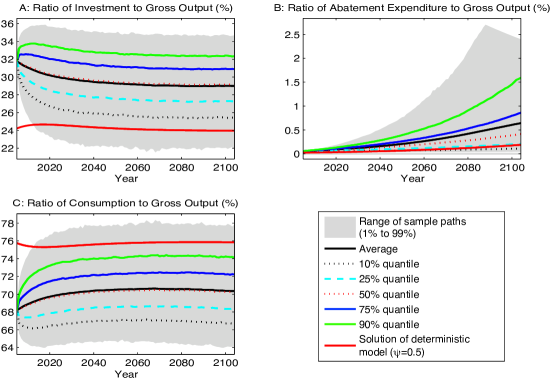
Figure 1: Simulation results of the stochastic growth benchmark—ratios to gross world output

Panel C presents quite the opposite statistical picture for $C_{t}/\mathcal{Y}_{t}$. We see that with more than 90 percent probability $C_{t}/\mathcal{Y}_{t}$ will be lower than in a purely deterministic model and that toward the end of this century $C_{t}/\mathcal{Y}_{t}$ appears to stabilize at about 70 percent; a reduction of about 6 percent over the deterministic model. Overall, this reduction is not fully offset by higher capital investments and, as panel B indicates, that difference is allocated to expenditures on abatement of emissions. We find that the latter, which is denoted by $\Psi_{t}/\mathcal{Y}_{t}$, is generally quite low and does not exceed 0.2 percent in this century in the deterministic case. Yet, as the black solid line in panel B indicates, there is a 50 percent probability that the expenditures on emissions abatement will be at least three times higher by the year 2100 when growth is modeled stochastically. Furthermore, with more than 20 percent probability more than 1 percent of gross world output should be devoted to mitigation by the year 2100.

The optimal allocation of gross world output is a portfolio choice problem where abatement expenditures are a form of investment. Thus, savings are split into investing in the capital stock or reducing the capital stock. In sum, Figure 1 indicates that the inclusion of stochastic growth with persistence will have significant impacts on the optimal allocation of gross world output and that deterministic specifications and, most likely, even certainty equivalent formulations will fail to account for these impacts.

We have investigated the dynamics of the economic variables, now we study the relation between them. Table 2 reports the correlation matrices of the growth rates of five economic variables: gross world output, consumption, capital investment, abatement expenditure, and the social cost of carbon, in 2020 and 2100. We see that all reported correlation numbers are almost the same in 2020 and 2100. Moreover, the growth of abatement expenditure is almost independent of all the other four variables, the growth of both consumption and capital investment are highly correlated with the growth of gross output, and the growth of the social cost of carbon is also highly correlated with the growth of consumption.

	Correlation at 2020					Correlation at 2100
	$g_{\mathcal{Y},t}$	$g_{\mathcal{C},t}$	$g_{I,t}$	$g_{\mathcal{\varPsi},t}$	$g_{\mathrm{SCC},t}$	$g_{\mathcal{Y},t}$	$g_{\mathcal{C},t}$	$g_{I,t}$	$g_{\mathcal{\varPsi},t}$	$g_{\mathrm{SCC},t}$
$g_{\mathcal{Y},t}$	1	0.90	0.95	-0.02	0.77	1	0.90	0.94	-0.00	0.78
$g_{\mathcal{C},t}$	0.90	1	0.71	-0.02	0.91	0.90	1	0.70	-0.00	0.91
$g_{I,t}$	0.95	0.71	1	-0.02	0.58	0.94	0.70	1	0.00	0.57
$g_{\mathcal{\varPsi},t}$	-0.02	-0.02	-0.02	1	-0.01	-0.00	-0.00	0.00	1	0.00
$g_{\mathrm{SCC},t}$	0.77	0.91	0.58	-0.01	1	0.78	0.91	0.57	0.00	1

Table 2: Correlation between the growth rates of gross world output $\mathcal{Y}_{t}$, consumption $C_{t}$, investment $I_{t}$, abatement expenditure $\Psi_{t}$, and the social cost of carbon $\mathrm{SCC}_{t}$

We next study how the stochastic growth specification affects the dynamics of the social cost of carbon, the carbon tax, the emission control rate, and the two most important climate states: atmospheric carbon concentration and surface temperature.

We first consider panel C in Figure 2 which shows the distribution of the rate of emission control. We observe that with 90 percent probability, the stochastic growth representation implies a higher emission control rate until the middle of this century and that by 2100 the probability is reduced to 75 percent. The generally much higher emission control rate is directly linked to the increased share of abatement expenditures to gross world output. The latter occurs because the prospects of much higher growth translate to expectations of increasing gross emissions, which in turn increase the atmospheric carbon stock and ultimately enhance global warming with its exponentially increasing damage to gross world output.

Both panels D and E indicate that on average the stochastic growth representation will lead to a slightly lower accumulation of carbon in the atmosphere and also have a small cooling effect on temperature. However, mostly due to the uncertainty about economic growth over the present century, we see that the range of atmospheric temperature in 2100 is about 1 degree Celsius, suggesting a large uncertainty about the extent of global warming and its impacts on the world economy and the environment. In fact, at the 2009 Copenhagen climate convention most climate scientists agreed that keeping changes in temperature levels below 2 degrees Celsius is necessary to prevent climate change from having dangerous impacts.

Figure 2: Simulation results of the stochastic growth benchmark—climate system and policies

As explained earlier, the monetized impacts of climate change are expressed by the social cost of carbon which we depict in panel A (on log₁₀ scale). The optimal initial social cost of carbon is $61 per ton of carbon, about 65 percent higher than in a purely deterministic economy, such as that assumed in Nordhaus (2008), whose study is currently being used for the design of climate policy in the United States, and to which our model compares when we eliminate the uncertainty about growth. Furthermore, the range resulting from the 1 percent and 99 percent quantiles of the simulation increases substantially over time. Here, the social cost of carbon in 2100 varies from $65 per ton of carbon to $1,200 per ton of carbon and even the 10 percent and 90 percent quantiles in 2100 show a range of $125 per ton of carbon to $660 per ton of carbon.

A major observation of our analysis is that by the year 2100 about 3 percent of our model runs produce a carbon tax (panel B) much lower than the social cost of carbon. This coincides with the simulation paths for which the emission control rate hits its upper bound of 100 percent, implying that it is optimal to have zero emissions. We obtain the social cost of carbon from the optimization framework of a social planner, and a (Pigovian) carbon tax policy in this case could be implemented to equate private and social costs of carbon in the absence of other market imperfections, and thus achieve the first best policy. When the emission control rate is at its limit, the carbon tax needs only to be large enough to eliminate all emissions, but as our results show it can be far less than the social cost of carbon. The gap between the carbon tax and the social cost of carbon can be large, with the largest carbon tax in 2100 less than $1,000 per ton of carbon while the largest social cost of carbon is $2,000 per ton of carbon among the 10,000 simulations.

A direct implication of this finding for climate policy is that with more than 3 percent probability, mitigation policies will reach the limit of their effectiveness and since the social cost of carbon will be much larger than the carbon tax can internalize, alternative policies such as carbon removal and storage or solar geoengineering technologies may become competitive.

Our findings point to one very important fact: there is great uncertainty about all aspects of the combined economic and climate system. For many variables, the mean value at each point in time is close to the solution of the purely deterministic model. Tracking the mean is all one can ask of any deterministic model, and in that sense deterministic models can be successful. However, there is great uncertainty about the future value of each key variable. This fact is of particular importance for understanding the social cost of carbon. The social cost of carbon is the marginal cost of extra carbon in terms of wealth, making it the marginal rate of substitution between mitigation expenditures and investment expenditures in physical capital. At the margin, those two uses of savings have different impacts on future economic variables, making allocation decisions between mitigation and investment essentially a portfolio choice problem; a large social cost of carbon represents the amount of investment in new capital that one is willing to sacrifice to reduce carbon emissions by a gigaton.

6.2 Uncertainty Quantification for Preference Parameters

Empirical work suggests plausible values for $\psi$ and $\gamma$, but the data do not give us precise values for the key parameters. A basic method in the uncertainty quantification literature is to recompute the social cost of carbon over a range of parameter choices that reflect the range of economic analyses. We examine different values of $\psi$ and $\gamma$ to determine the sensitivity of the social cost of carbon to alternative preference specifications. Each example will differ from the stochastic growth benchmark only in the preference specification, as we will always use the benchmark stochastic growth productivity process. Thus, the following results are comparative dynamics only for changes in $\psi$ and $\gamma$.

Our sensitivity analysis will look only at the social cost of carbon at the initial time. Simulations show that the dynamic stochastic process for the social cost of carbon is qualitatively similar to the stochastic growth benchmark in all cases. The social cost of carbon at the initial time can be thought of as the initial value for the social cost of carbon process, which is volatile for any choice of preference parameters. Table 3 lists the initial optimal social cost of carbon from our model under stochastic growth assuming the values of the elasticity of inter-temporal substitution to be $\psi=0.5$, 0.75, 1.25, 1.5, and 2.0, and the risk aversion parameter to be $\gamma=0.5,$ 2, 6, 10, and 20. Recall that, in our benchmark example with $\psi=1.5$ and $\gamma=10$, the optimal initial social cost of carbon is $61 per ton of carbon. Table 3 indicates that for our benchmark case with $\gamma=10$ the social cost of carbon is almost invariant to alternative specifications of $\psi$, while keeping $\psi=1.5$, the social costs of carbon at the initial time will be smaller for higher levels of $\gamma$.

$\psi$	Deterministic	$\gamma$
	Growth Case	0.5	2	6	10	20
$0.5$	37	35	39	52	61	69
$0.75$	54	53	55	58	60	62
$1.25$	82	83	77	65	61	56
$1.5$	94	95	85	68	61	55
$2.0$	111	115	97	71	62	54

Table 3: Initial social cost of carbon ($ per ton of carbon) under stochastic growth

More generally, Table 3 shows that the social cost of carbon is sensitive to the preference parameters, ranging from $35 (in the case of $\psi=0.5$ and $\gamma=0.5$) to $115 (in the case of $\psi=2$ and $\gamma=0.5$). We see that when the inter-temporal elasticity of substitution ($\psi$) is less than unity, a higher $\gamma$ will imply a higher social cost of carbon. However, when the inter-temporal elasticity of substitution is larger than 1, the social cost of carbon is decreasing in $\gamma$. Moreover, when $\gamma\leq 6$ a higher inter-temporal elasticity of substitution implies a higher social cost of carbon, but for $\gamma=20$ the opposite is the case. An increase in the inter-temporal elasticity of substitution reduces the preference for consumption-smoothing but that tells us little about the social cost of carbon. The social cost of carbon is the value of mitigation expenditures relative to the value of capital investment, both of which are chosen. Our results show that the interplay between the inter-temporal elasticity of substitution and the risk aversion parameter in our model with stochastic growth is nontrivial for the social cost of carbon.

From Table 3, we see also that when $\gamma\geq 2$, a higher volatility of uncertain economic growth implies a lower initial social cost of carbon for cases with $\psi>1$, or implies an higher initial social cost of carbon for cases with $\psi>1$ (as the volatility of the deterministic case is zero). The outcomes of general equilibrium come from a mix of income and price effects, making it difficult to arrive at simple explanations. Our sensitivity analysis enables us to examine quantitatively the impact of alternative parametric assumptions.

Tables 4 and 5 report the sensitivity of the initial ratios of capital investment to gross world output ($I_{t}/\mathcal{Y}_{t}$) and abatement expenditure to gross world output ($\Psi_{t}/\mathcal{Y}_{t}$) respectively, for the combinations of $\gamma$ and the inter-temporal elasticity of substitution.

For example, when $\psi=1.5$ and $\gamma=10$, initial $I_{t}/\mathcal{Y}_{t}$ is 0.317 and $\Psi_{t}/\mathcal{Y}_{t}$ is $5.5\times 10^{-4}$. From Table 4 we see that capital investment is increasing in $\gamma$. Table 5 displays the same pattern for abatement expenditure as that displayed for the social cost of carbon in Table 3: When the inter-temporal elasticity of substitution is less than 1, a higher $\gamma$ will imply a higher ratio; when the inter-temporal elasticity of substitution is larger than 1, the ratio is decreasing in $\gamma$; and a higher $\psi$ does not necessarily imply a higher or lower ratio of abatement expenditure to gross world output.

$\psi$	Deterministic	$\gamma$
	Growth Case	0.5	2	6	10	20
$0.5$	0.242	0.240	0.249	0.272	0.291	0.321
$0.75$	0.259	0.257	0.265	0.285	0.299	0.318
$1.25$	0.278	0.276	0.286	0.303	0.312	0.322
$1.5$	0.284	0.283	0.293	0.310	0.317	0.324
$2.0$	0.293	0.293	0.305	0.322	0.328	0.331

Table 4: Initial ratio of capital investment to gross world output under stochastic growth

$\psi$	Deterministic	$\gamma$
	Growth	0.5	2	6	10	20
$0.5$	$2.6(-4)$	$2.4(-4)$	$2.9(-4)$	$4.5(-4)$	$5.7(-4)$	$7.1(-4)$
$0.75$	$4.7(-4)$	$4.7(-4)$	$4.9(-4)$	$5.5(-4)$	$5.7(-4)$	$5.9(-4)$
$1.25$	$9.1(-4)$	$9.1(-4)$	$8.4(-4)$	$6.5(-4)$	$5.5(-4)$	$5.0(-4)$
$1.5$	$1.1(-3)$	$1.1(-3)$	$9.8(-4)$	$6.8(-4)$	$5.5(-4)$	$4.8(-4)$
$2.0$	$1.4(-3)$	$1.6(-3)$	$1.2(-3)$	$7.3(-4)$	$5.9(-4)$	$4.7(-4)$

Table 5: Initial ratio of abatement expenditure to gross world output under stochastic growth. Note that $a(-n)$ represents $a\times 10^{-n}$

We also study the effects of alternative preference specifications on the dynamics (level and distribution) of the social cost of carbon and per capita consumption growth. Table 6 lists these effects for only the extreme parameter cases of our simulations, which are $\psi=0.5$ or 2, and $\gamma=0.5$ or 20. First, we verify the statistical results of per capita consumption over the large range of preference parameters. Its mean growth rate is quite stable over this century, ranging from 1.1 percent to 1.4 percent per year, close to that of the benchmark case shown in Table 1. We also report the other statistics used in Table 1 such as the statistics of $\Lambda$ and $\sigma(\epsilon)$ for the lag-1 autoregression (18). These numbers show that a smaller $\psi$ will produce a larger volatility for the per capita consumption growth $g_{c}$. Furthermore, the volatility of $g_{c}$ is quite invariant to different values of the risk aversion parameter. In addition, all the cases show the mean-reverting property of the consumption growth: the 95% confidence level of $\Lambda$ is always below one (for lower $\psi$ levels, $g_{c}$ has a smaller $\Lambda$, implying a faster reverting rate), and its mean and standard deviation are almost independent of time for each reported $(\psi,\gamma)$ combination.

Regarding the sensitivity of the social costs of carbon, we recall from Figure 2 of our benchmark parameter case that the social cost of carbon is highly volatile. Here, we show that this high volatility is also persistent when we assume alternative preference specifications. More precisely, the mean and—in particular—the standard deviation of $\log_{10}(\mathrm{SCC})$ are increasing over time. Furthermore, the mean of $\Lambda$ is not less than 1, implying non-stationarity of $\log_{10}(\mathrm{SCC})$.

	$\log_{10}(\mathrm{SCC})$				$g_{c}$
$\psi$	$0.5$		$2$		$0.5$		$2$
$\gamma$	$0.5$	$20$	$0.5$	$20$	$0.5$	$20$	$0.5$	$20$
mean at 2020	1.632	2.045	2.171	1.858	0.011	0.014	0.013	0.014
mean at 2050	1.878	2.369	2.372	2.069	0.013	0.013	0.013	0.013
mean at 2100	2.211	2.763	2.656	2.347	0.012	0.012	0.012	0.012
standard deviation at 2020	0.068	0.113	0.097	0.074	0.036	0.035	0.023	0.021
standard deviation at 2050	0.181	0.251	0.189	0.161	0.037	0.037	0.023	0.022
standard deviation at 2100	0.283	0.370	0.282	0.249	0.039	0.039	0.025	0.023
mean of $\Lambda$	1.008	1.005	1.000	1.005	0.100	0.091	0.584	0.708
standard error of $\Lambda$	0.012	0.014	0.017	0.014	0.116	0.118	0.148	0.101
mean of $\sigma(\epsilon)$	0.009	0.016	0.017	0.011	0.036	0.036	0.018	0.015
standard error of $\sigma(\epsilon)$	0.001	0.001	0.001	0.001	0.003	0.003	0.003	0.002

Table 6: Statistics of the social cost of carbon (on log₁₀ scale) and per capita consumption growth $g_{c}$ for four extreme cases of preference parameters

6.3 Impact of Growth Parameters

The deterministic productivity trend $A_{t}$ has a growth rate $\alpha_{1}\exp(-\alpha_{2}t$) at time $t$ from Equation (2). It has two important parameters: the initial growth rate, $\alpha_{1}$, and the decline rate of the growth of the productivity trend, $\alpha_{2}$, with their default values 0.0092 and 0.001 respectively. We next carry out a sensitivity analysis on them by letting $\alpha_{1}=0$ (the growth of the productivity trend is 0, i.e., $A_{t}\equiv A_{0}$) or $\alpha_{2}=0$ (the growth of the productivity trend is constant, i.e., $A_{t}=A_{0}\exp\left(\alpha_{1}t\right)$ with $\alpha_{1}=0.0092$).

Table 7 lists the simulation statistics of the social cost of carbon and per capita consumption growth for the two cases described above, with all remaining parameters of the stochastic growth benchmark case unchanged (we also list the statistics for the stochastic growth benchmark case in which $A_{t}=0.0092e^{-0.001t}$). When $A_{t}$ is a constant (i.e., $\alpha_{1}=0$), the initial-time social cost of carbon is only $39 per ton of carbon ($\log_{10}(\mathrm{SCC})=1.591$), much less than the $61 per ton of carbon of the stochastic growth benchmark case. From Table 7 we find that the values of $\alpha_{1}$ and $\alpha_{2}$ (different deterministic productivity trends) change the means of consumption growth $g_{c}$, but have little impact on the standard deviation, $\Lambda$, and $\sigma(\epsilon)$. Nevertheless, we still observe the mean-reverting property of consumption growth. In contrast, the different deterministic productivity trends do change both the mean and the standard deviation of $\log_{10}(\mathrm{SCC}_{t})$. A smaller productivity trend $A_{t}$ leads to a smaller mean and also a smaller standard deviation of $\log_{10}(\mathrm{SCC}_{t})$. The non-stationarity of $\log_{10}(\mathrm{SCC})$ still exists for both cases as their means of $\Lambda$ are still larger than 1.

	$\log_{10}(\mathrm{SCC})$			$g_{c}$
growth of $A_{t}$	0	0.0092	$0.0092e^{-0.001t}$	0	0.0092	$0.0092e^{-0.001t}$
initial-time solution	1.591	1.792	1.785	—	—	—
mean at 2020	1.662	1.934	1.924	0.002	0.014	0.014
mean at 2050	1.714	2.167	2.153	0.000	0.013	0.013
mean at 2100	1.703	2.490	2.457	-0.000	0.013	0.012
standard deviation at 2020	0.096	0.086	0.087	0.024	0.024	0.024
standard deviation at 2050	0.215	0.183	0.184	0.025	0.025	0.024
standard deviation at 2100	0.393	0.278	0.279	0.025	0.025	0.025
mean of $\Lambda$	1.005	1.003	1.003	0.431	0.458	0.458
standard error of $\Lambda$	0.016	0.015	0.015	0.149	0.134	0.135
mean of $\sigma(\epsilon)$	0.017	0.013	0.013	0.021	0.021	0.021
standard error of $\sigma(\epsilon)$	0.001	0.001	0.001	0.002	0.002	0.002

Table 7: Statistics of the social cost of carbon (on $\log_{10}$ scale) and per capita consumption growth $g_{c}$ for cases with different rates of growth in the deterministic productivity trend

To better understand the mechanism driving this result, recall Equation (17) for the social cost of carbon and the fact that the social cost of carbon is itself a ratio of the negative shadow price of carbon and the shadow price of capital. Thus, any change in the risk structure will affect both shadow prices. Here, a lower expected growth rate (as the trend is set to zero) will reduce the expectation of the level of the capital stock when compared to our stochastic growth benchmark, since the stochastic factor productivity growth process is the same in both cases. At the same time, since the economy now grows without a positive trend of about 0.92 percent per year, gross emissions, which are proportional to gross world output, will also grow less by that amount. Consequently, less carbon will accumulate in the atmosphere at each point in time. A careful comparison of these effects is difficult in general equilibrium, but we note here that the value function is concave in capital and convex in the carbon stock, leading to the combined effect of reducing the social cost of carbon.

In the $\alpha_{1}=0$ case there is only a stochastic component of growth. As a consequence, the expectation of the mean of $g_{c}$ is close to zero over the 21st century, while the standard deviation of $g_{c}$ and its residual is close to that of the stochastic growth benchmark case with deterministic trend.

For the case $\alpha_{2}=0$, the initial-time social cost of carbon is $62 per ton of carbon ($\log_{10}(\mathrm{SCC})=1.792$), only slightly larger than the stochastic growth benchmark. A model version with $\alpha_{2}=0$ actually implies a higher deterministic trend as the reduction in the trend is set to zero. As a consequence, the opposite effects of those of the $\alpha_{1}=0$ case are observed. The expected social cost of carbon is also higher throughout the rest of this century, while the standard deviation of the social cost of carbon and its residuals is similar to that of the stochastic benchmark case. Similar insights are obtained from studying the per capita consumption growth rate of the $\alpha_{2}=0$ case.

7 Social Cost of Carbon with (only) Stochastic Climate Tipping

We next study how a tipping element in the climate system may affect the social cost of carbon in the absence of any economic uncertainty. First, we present a Markov chain specification of a representative climate tipping element. Based on our calibration, we then set up a benchmark parameter specification and study optimal climate policy; we call this our climate tipping benchmark. In a final step we present an extensive multidimensional sensitivity analysis with broad ranges of each of the parameters. In light of the numbers provided in the few studies available, we conclude that the impact from potential tipping point events should be carefully assessed. Appendix D presents a more detailed derivation of our parameter choices.

7.1 A Markov Chain Specification of the Climate Tipping Process

As described in Section 4.3, we have a pre-tipping stage where $J_{t}=0$ until the climate tipping process begins, followed by several stages of increasing damage. We assume that the probability function of staying in the pre-tipping stage is $p_{1,1,t}$, given by the formula (15). The hazard rate parameter $\lambda$ together with the temperature process determines the duration of the pre-tipping stage.

We assume that the long-run post-tipping damage level, denoted $\mathcal{J}_{\infty}$, is uncertain. We assume that we do not know $\mathcal{J}_{\infty}$ until the climate tipping process is triggered. This is a stark simplification, but it does allow us to distinguish the expected duration of the post-tipping process, $\overline{\mathcal{D}}$, which is always known, from the uncertainty about the ultimate damage level. The fact that the uncertainty about $\mathcal{J}_{\infty}$ is resolved when the climate tipping process is triggered allows us to make statements about the relative impact of the hazard rate of the tipping point event, the expected duration of the post-tipping process, and the mean and variance of $\mathcal{J}_{\infty}$. The unconditional mean of $\mathcal{J}_{\infty}$ is denoted $\overline{\mathcal{J}}_{\infty}$, and the variance of $\mathcal{J}_{\infty}$ is $q\overline{\mathcal{J}}_{\infty}^{2}$, where $q$ is called the “mean squared-variance ratio”. The ratio $q$ is analogous to the square of the Sharpe ratio, a concept used in portfolio theory, and arises naturally in our discussion of results.

In our examples, we assume that there are three possible post-tipping damage levels in the long run. For each long-run damage level, the tipping process moves through five more stages, the fifth being the final state, and each transition occurs at the same fixed rate. Thus, if $\overline{\mathcal{D}}$ is the expected duration of the post-tipping process, then each transient stage has the expected duration $\overline{D}_{i}=\overline{\mathcal{D}}/4$ and all transitions have an exponential distribution, implying $p_{i,i+1,t}=\exp\left(-4/\overline{\mathcal{D}}\right)$. Experimentation indicated that five tipping stages is adequate to approximate processes with more states at relatively low computational costs. These specifications imply a total of sixteen possible values for $J_{t}$, the pre-tipping stage, and five post-tipping stages or each of the three realizations of long-run damage. The complete mathematical description of $J_{t}$ is contained in Appendix D.

7.2 The Stochastic Climate Tipping Benchmark

We choose parameter values that are roughly the average of the range of opinions in the literature. More precisely, the climate tipping benchmark case assumes $\lambda=0.0035$, $\overline{\mathcal{J}}_{\infty}=0.05$, $q=0.2$, and $\mathcal{\overline{\mathcal{D}}}=50$. The choice of $\lambda=0.0035$ implies that the conditional annual probability of tipping increases by 0.35 percent for a warming of 1 degree Celsius. The Epstein–Zin preference parameters in the climate tipping benchmark case are again $\psi=1.5$ and $\gamma=10$.

We first study the effect of a possible climate tipping point on the optimal allocation of gross world output to capital investment, consumption, and abatement expenditures. Figure 3 shows the dynamics of the ratio of consumption to gross world output ($C_{t}/\mathcal{Y}_{t}$), the ratio of capital investment to gross world output ($I_{t}/\mathcal{Y}_{t}$), and the ratio of abatement expenditure to gross world output ($\Psi_{t}/\mathcal{Y}_{t}$) respectively.

Figure 3: Simulation results for the stochastic climate tipping benchmark—ratios to gross world output

As a general finding, we first note that the absence of stochastic growth clearly reduces the range of the distribution of all three ratios. Now, the climate tipping point risk is the sole component by which output can be reduced and our calibration of post-tipping damage levels is much lower that the possible change in gross world output due to stochastic growth with a long-run persistence.

We see that accounting for a climate tipping element implies throughout this century a higher share of output be devoted to capital investment (about 3 percent on average) and abatement expenditures, and a smaller share be allocated to consumption (about 3 percent on average). Thus, the optimal policy for addressing the tipping point risks implies a reallocation of gross output away from consumption and toward a precautionary buildup of the capital stock and simultaneous reductions in emissions.

The sign of these effects comes from the the income effect of the threat of a tipping point, but here we also point out that the magnitude of these changes relative to the expected value of damage from tipping is high if one believes that future consumption should be discounted at a market interest rate of about 5 percent. For example, $1 in 2150 is worth about $0.0014 in 2015 if it is discounted at a 5 percent rate per year.

We next consider the implications of a climate tipping point on the dynamics of the social cost of carbon, the carbon tax, the emission control rate, and the two most important climate states (atmospheric carbon concentration and surface temperature) respectively. Figure 4 shows the results of 10,000 simulation paths over the first 200 years for these variables and we use the same color and line conventions as in the previous figures.

Because of the existence of climate tipping risk and Epstein–Zin preferences, the model version with stochastic climate tipping is expected to result in a more intense climate policy compared to that of a deterministic model. In fact as panel C in Figure 4 shows, the optimal emission control rate follows a pattern related to that of the abatement expenditures in the previous figure. Throughout this century it is optimal to more than double the emission efforts as a response to the threat of a tipping point in the climate.

These immense emission reductions of our climate tipping benchmark case imply a strict reduction of atmospheric carbon concentrations (panel D) compared to that of the deterministic model. The resulting path of surface temperature (panel E) corresponds to the temperature paths from the lowest of the most recent emission scenarios used by IPCC (2013), implying a peak temperature increase before 2100 of around 2 degrees Celsius and a decline afterward.

A striking result in panel A of Figure 4 is the initial social cost of carbon of $189 per ton of carbon, a large increase over the $38 per ton of carbon resulting from a model specification which ignores the stochastic nature of the climate. To underline the significance of this major increase in the social cost of carbon, recall our rather conservative assumptions on the nature of the tipping point processes: we assume an expected duration of the tipping process of 50 years, an expected post-tipping damage of 5 percent, and a mean squared-variance ratio of 0.2. As can be seen from the blue dashed line, these assumptions indicate that there is a 75 percent probability that a tipping process will not be triggered before 2150. Yet today’s optimal social cost of carbon is $189 per ton of carbon, five times the value obtained from a model run in which the climate tipping point is ignored. This strongly suggests that analyses of climate policy which simply ignore the potential of abrupt changes to the climate system—as does the current United States government study (Interagency Working Group on Social Cost of Carbon, 2010)—are significantly underestimating the social cost of carbon.

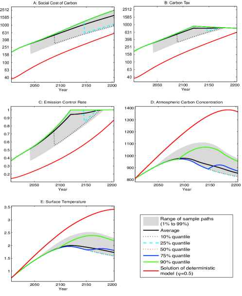
Figure 4: Simulation results for the stochastic climate tipping benchmark—climate system and policies

The dynamics of the distribution of the social costs of carbon indicate that by 2100 the expected social cost of carbon is about $630 per ton of carbon, which is almost four times the $160 per ton of carbon obtained from a deterministic model. Furthermore, the expected social cost of carbon in year 2200 is about $1,700 per ton of carbon but our simulations produce a range from about $1,000 per ton of carbon to $2,500 per ton of carbon.

Related to the analysis in the previous section, we also note here that by the year 2125 some of our 10,000 simulated paths will produce a carbon tax which is less than the social cost of carbon, indicating that the opportunities to address the climate externality are exhausted as mitigation may not be larger than 100 percent. In fact, it appears that, with a slightly higher than 75 percent probability, mitigation policies will reach their limits of effectiveness by 2125 and alternative carbon management options might be useful.

7.3 Uncertainty Quantification for the Climate Tipping Process

We next examine how the initial social cost of carbon is affected by parameter uncertainty in the climate tipping process by recomputing the social cost of carbon over a range of parameter choices that reflect scientific opinions. We examine the six-dimensional collection (2,430 cases) of parameter values defined by the tensor product of the following finite sets:

$$\lambda\in\left\{0.0025,0.0035,0.0045\right\},\;\;\;\;\;\;\;\overline{\mathcal{J}}_{\infty}\in\left\{0.025,0.05,0.10\right\},\;\;\;\;\;\;\;q\in\{0,0.2,0.4\},$$

$$\psi\in\{0.5,0.75,1.25,1.5,2.0\},\;\;\;\;\;\;\;\gamma\in\{0.5,2,6,10,14,20\},\;\;\;\;\;\;\;\overline{\mathcal{D}}\in\{5,50,200\}.$$

We compute the social cost of carbon at the initial time for all the 2,430 cases and Table 8 presents the initial social cost of carbon for some of the representative cases. For example, when $\lambda=0.0035$, $\overline{\mathcal{J}}_{\infty}=0.05$, $q=0.2$, and $\mathcal{\overline{\mathcal{D}}}=50$ (i.e., the last row in Table 8) the initial social cost of carbon is $189 per ton for $\psi=1.5$ and $\gamma=10$. The value of the social cost of carbon with the climate tipping process is always greater than in the deterministic case in which the climate tipping process is ignored. This is expected since the tipping element increases future possible damage.

Table 8 also shows that the social cost of carbon is larger for a higher inter-temporal elasticity of substitution $\psi$, and a higher value of the risk aversion parameter $\gamma$. Furthermore, we observe that the initial-time social cost of carbon increases with higher (present-discounted) expected damages from the climate tipping process, which can be caused by a higher mean damage level ($\overline{\mathcal{J}}_{\infty}$), a higher hazard rate parameter ($\lambda$), a shorter expected duration of the tipping process ($\overline{\mathcal{D}}$) , or by a higher mean squared-variance ratio of the expected damage level ($q$). As mentioned earlier, our specification of a climate tipping point in an economic growth model is unique by the standards of how climate scientists view the nature of climate tipping points (e.g., Lenton and Ciscar 2013). In the nomenclature of our model, previous studies often assume $\overline{\mathcal{J}}_{\infty}>0.15$ (sometimes even 0.3), $\mathcal{\overline{\mathcal{D}}=}1$, and the implied $\lambda$ is much higher than 0.0045. The insights obtained using models with such extreme and in some case wrong assumptions should be assessed with special care.

				Social cost of carbon ($\mathrm{SCC}$)
$\lambda$	$\overline{\mathcal{J}}_{\infty}$	$\mathcal{\overline{\mathcal{D}}}$	$q$	$\psi=0.5$			$\psi=1.5$
				$\gamma=0.5$	$\gamma=10$	$\gamma=20$	$\gamma=0.5$	$\gamma=10$	$\gamma=20$
0.0025	0.025	5	0	43	44	45	128	131	135
			0.4	43	45	46	128	134	142
		200	0	39	39	39	110	111	112
			0.4	39	39	39	110	112	114
	0.10	5	0	65	83	110	260	364	482
			0.4	65	103	194	261	467	722
		200	0	47	50	54	170	195	230
			0.4	47	52	62	171	224	343
0.0045	0.025	5	0	47	49	50	147	150	154
			0.4	47	50	52	147	155	164
		200	0	40	41	41	119	120	121
			0.4	40	41	41	119	121	124
	0.10	5	0	85	109	143	369	480	584
			0.4	85	140	252	370	586	817
		200	0	54	58	63	222	259	305
			0.4	54	62	76	223	306	445
0.0035	0.05	50	0.2	48	52	55	171	189	216

Table 8: Initial social cost of carbon ($ per ton of carbon) with stochastic climate tipping

Here, the increase in the social cost of carbon relative to $q$ is very minor when $\gamma$ or $\overline{\mathcal{J}}_{\infty}$ is small (a small $\overline{\mathcal{J}}_{\infty}$ implies a much smaller variance of the uncertain, final, post-tipping damage level which is equal to $q\overline{\mathcal{J}}_{\infty}^{2}$), particularly for large expected durations. However, it becomes more visible for larger values of $\gamma$. Therefore, the effect of rising uncertainty about future damage from abrupt climate change is amplified with higher values of the risk aversion parameter. In models assuming separable preferences, it is only the mean of the uncertain damage, and not its variance, that affects the social cost of carbon.

Keeping our climate tipping benchmark preference parameters, the most pessimistic description of the tipping point process will imply today’s optimal social cost of carbon to be $568 per ton of carbon, while increasing the risk parameter to 20 would further increase today’s social cost of carbon to $817 per ton of carbon.

In addition, from the results of all the 2,430 cases, we found that there exists one common pattern: the initial social cost of carbon is linear in $q$. Figure 5 shows the numbers for the social cost of carbon for various values of $\gamma$ and $q$, when $\psi=1.5$, $\lambda=0.0035$, $\overline{\mathcal{J}}_{\infty}=0.05$, and $\overline{\mathcal{D}}=50$. Other cases have the same qualitative pattern, so we omit them here. In Figure 5, the blue line, the black line, the red line, and the green line represent the case of $\gamma=0.5$, 2, 6, 10, 14, and 20 respectively. We see that all these lines are straight, and that a higher $\gamma$ implies a greater slope, meaning that it is more sensitive to the variance of the uncertain damage level.

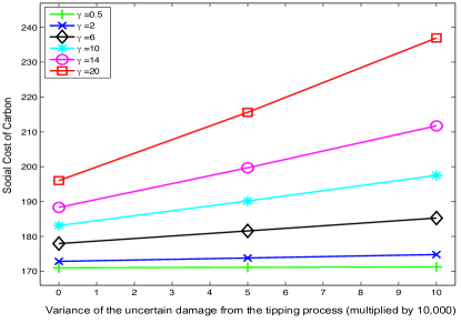
Figure 5: Sensitivity of the social cost of carbon to the risk-aversion parameter and uncertainty regarding post-tipping damage

This is not surprising since it fits into the logic of the basic consumption-based capital asset pricing model (Lucas 1978) which tells us that the price of risk is related to its covariance with the aggregate endowment. Since the magnitude of the damage is proportional to output, the damage is strongly related to output; in fact, in this case the climate damage is the only stochastic element of output conditional on the tipping event. Therefore, the correlation is unity and the social cost of carbon has a price of risk component which is linear in the variance of the uncertain damage level.

Note that the social cost of carbon increases as the variance of the uncertain damage level increases. One interpretation of variance is that it represents our ignorance of the consequences of an unfolding tipping process. With that interpretation, the horizontal difference represents the decline in the social cost of carbon that would result if we carried out more scientific research and reduced the uncertainty regarding the post-tipping damage level. This observation shows that our model could be used to identify the value of reducing uncertainty and to indicate which kinds of scientific studies would be the most valuable to pursue. This is a point left for further development in future studies.

8 Social Cost of Carbon with Stochastic Growth & Climate Tipping

The previous two sections have examined the impacts on the social cost of carbon from stochastic growth and stochastic climate tipping, both in isolation. The real world system includes both uncertainties and this section presents the results of our model in the presence of long-run risk in both economic growth and in the climate tipping process. The optimal policy will now have to balance the need to delay the triggering of the tipping point process with the accumulation of additional capital in the face of stochastic growth, and with the desire to smooth our consumption patterns. We study a stochastic growth and climate tipping benchmark case of parameter specification and carry out a sensitivity analysis.

8.1 The Stochastic Growth & Climate Tipping Benchmark

We use $\psi=1.5$, $\gamma=10$, $\lambda=0.0035$, $\overline{\mathcal{J}}_{\infty}=0.05$, $q=0.2$, and $\mathcal{\overline{\mathcal{D}}}=50$ for the stochastic growth and climate tipping benchmark. Figure 6 shows the results of 10,000 simulation paths over the first 100 years for dynamics of the social cost of carbon, the carbon tax, and the ratio of social cost of carbon to gross world output respectively. Other variables such as capital, consumption and its growth, atmospheric carbon concentration, and surface temperature have pictures visually similar to the corresponding pictures in Figures 2 and 4, so we omit them. We use the same line and color types as in previous figures.

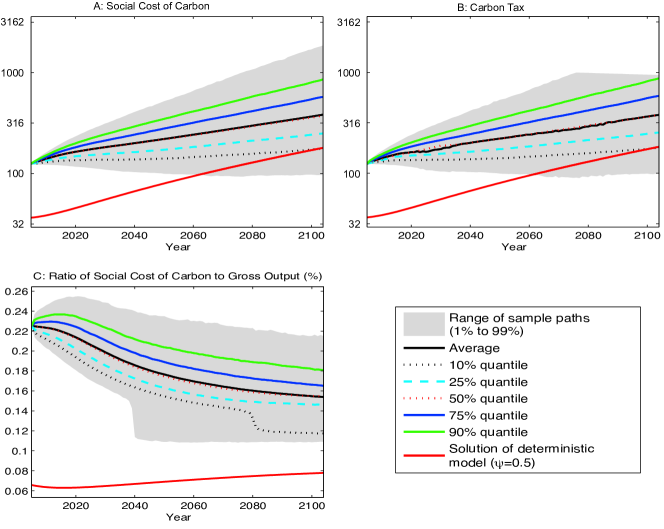
Figure 6: Simulation results for stochastic growth and climate tipping benchmark

We first study the social cost of carbon. Its initial-time level is $125 per ton of carbon and at 2100 the average (or expected) social cost of carbon is around $400 per ton of carbon. Thus, the path of the expected social cost of carbon falls between its paths obtained from our analyses of each risk component in isolation. At the initial time the social cost of carbon of $125 per ton of carbon is even exactly the average of the numbers obtained from the two cases of the previous sections ($61 per ton of carbon and $189 per ton of carbon). Compared to a deterministic model, which would ignore both risk components and have $\psi=0.5$, we find that the initial social cost of carbon increases by a factor of 3.2 and that with 90 percent probability the social cost of carbon will be significantly higher throughout this century.

The presence of both stochastic growth and climate tipping risk also increases the variance of the future social cost of carbon relative to the separate stochastic growth and climate tipping benchmarks. For example, the social cost of carbon in 2100 ranges from $100 per ton of carbon (the 1 percent quantile) to $1,700 per ton of carbon (the 99 percent quantile). The carbon tax, which we present in panel B, is also more likely to hit its upper bound after 2072 than in either of the single risk benchmarks. The combination of these risks implies that there is a probability of about 7 percent that mitigation policies will have reached the limit of their effectiveness by 2100.

Some recent research has argued for simple rules of thumb for the social cost of carbon. In particular, Golosov et al. (2014) set up a dynamic, forward-looking climate–economy model with logarithmic utility and full capital depreciation to argue that the optimal social cost of carbon is proportional to output. Barrage (2014) shows that the benchmark in Golosov et al. (2014) implies that the ratio of the social cost of carbon to decadal gross world output is $8\times 10^{-5}$ and constant over time with constant productivity growth, but that it increases over time for the productivity process in Nordhaus (2008), approaching $8\times 10^{-5}$ from below. Direct comparisons with deterministic models like those analyzed in Barrage (2014) are difficult. Nevertheless, for our stochastic growth and climate tipping benchmark case, we compute the ratio of the social cost of carbon to gross world output ($\mathrm{SCC}_{t}/\mathcal{Y}_{t}$), which we show in panel C in Figure 6.

First, we note that when compared to the deterministic model version, $\mathrm{SCC}_{t}/\mathcal{Y}_{t}$ is about three times larger at the initial time while at 2100 it is expected to be about twice as large. Second, we find that the expected $\mathrm{SCC}_{t}/\mathcal{Y}_{t}$ is decreasing over time by about 50 percent, and is thus not constant. Third, and most importantly, we find that the ratio of the social cost of carbon to gross world output is not close to any simple path, but is rather a stochastic process varying over the interval [0.00108, 0.00215] at year 2100 and over an even larger interval for the second half of this century. These results indicate that when there are multiple uncertainties, such as in the economic and climate systems, incorporating them into an integrated assessment model might lead to substantially different qualitative and quantitative results. In this example case, we find no useful, robust, dynamic relation between the social cost of carbon and gross world output.

8.2 Sensitivity of the Stochastic Growth & Climate Tipping Benchmark

We compute the sensitivity of the stochastic growth and climate tipping benchmark case to several parameters. Table 9 lists the initial social cost of carbon for selected combinations of the parameter values for sensitivity analysis. These parameters are the hazard rate $\lambda$, the post-tipping damage level $\overline{\mathcal{J}}_{\infty}$, the mean duration time of the tipping process $\mathcal{\overline{\mathcal{D}}}$, the mean squared-variance ratio $q$, the elasticity of inter-temporal substitution $\psi$, the risk aversion parameter $\gamma$, and the rate of persistence in the long-run risk of stochastic growth $r$.

					Social cost of carbon ($\mathrm{SCC}$)
$\lambda$	$\overline{\mathcal{J}}_{\infty}$	$\mathcal{\overline{\mathcal{D}}}$	$q$	$r$	$\psi=0.5$		$\psi=1.5$
					$\gamma=2$	$\gamma=10$	$\gamma=2$	$\gamma=10$
0.0035	0.05	50	0	0.775	55	112	155	116
0.0035	0.10	50	0	0.775	73	189	236	191
0.0045	0.05	50	0	0.775	59	123	170	128
0.0035	0.05	5	0	0.775	63	133	175	136
0.0045	0.10	5	0	0.775	102	293	318	274
0.0045	0.10	5	0.4	0.775	107	398	331	354
0.0035	0.05	50	0	0.5	53	84	162	133

Table 9: Initial social cost of carbon ($ per ton of carbon) under stochastic growth and climate tipping

For example, when $\psi=1.5$, $\gamma=10$, $\lambda=0.0035$, $\overline{\mathcal{J}}_{\infty}=0.05$, $q=0$, $\mathcal{\overline{\mathcal{D}}}=50$, and $r=0.775$ (the default values used in all of the previous examples), the initial social cost of carbon is $116 per ton of carbon. We compare this number to the $125 per ton of carbon of the stochastic growth and climate tipping benchmark case in Subsection 8.1 for which we set $q=0.2$. Thus, higher $q$ implies a higher initial social cost of carbon, which is consistent with our observations for cases with a stochastic climate tipping only, shown in Table 8. This is more clearly reflected by comparing the extreme cases of the fifth and sixth rows of Table 9 (with $\lambda=0.0045$, $\overline{\mathcal{J}}_{\infty}=10\%$, $\mathcal{\overline{\mathcal{D}}}=5$, and $r=0.775$): for every case of $(\psi,\gamma)$, the sixth row with $q=0.4$ has a larger social cost of carbon than the fifth row with $q=0$. Also, the range of the initial-time social cost of carbon is wide, from $53 per ton of carbon (the case with $\lambda=0.0035$, $\overline{\mathcal{J}}_{\infty}=0.05$, $\mathcal{\overline{\mathcal{D}}}=50$, $r=0.5$, $\psi=0.5$, and $\gamma=2$) to $398 per ton of carbon (the case with $\lambda=0.0045$, $\overline{\mathcal{J}}_{\infty}=0.10$, $\mathcal{\overline{\mathcal{D}}}=5$, $r=0.775$, $\psi=0.5$, and $\gamma=10$).

Moreover, some qualitative properties found in previous examples with only climate risk still hold. That is, a higher hazard rate parameter $\lambda$, a higher mean damage level $\overline{\mathcal{J}}_{\infty}$, a larger mean squared-variance ratio $q$, or a shorter expected duration $\mathcal{\overline{\mathcal{D}}}$ will lead to a higher social cost of carbon, although their quantitative values differ substantially.

However, the qualitative properties of the preference parameters ($\psi$ and $\gamma$) are nontrivial now: when $\psi=0.5$, a higher $\gamma$ always implies a higher social cost of carbon, and when $\psi=1.5$, the table shows that the effect of higher $\gamma$ on the social cost of carbon can be positive or negative. In most cases except the sixth row of Table 9, a higher $\gamma$ will have a smaller social cost of carbon, while the sixth row is averse. We also know from Table 8 that if the volatility of the economic risk goes to zero, then a higher $\gamma$ will have a higher social cost of carbon for any $\psi$. This is partially reflected in the last row of the table: when $\psi=1.5$ and $r=0.5$, the difference of the social cost of carbon between $\gamma=2$ and $\gamma=10$ is $162-133=$ $29 per ton of carbon. This number is less than the corresponding difference in the first data row with $\psi=1.5$ and $r=0.775$, which is $155-116=$ $39 per ton of carbon, because the volatility of the economic risk with $r=0.775$ is larger than that with $r=0.5$.

9 Conclusion

This study has presented DSICE, a computational framework for stochastic integrated assessment of issues related to the joint evolution of the economy and the climate. We analyzed the optimal level and dynamic properties of the social cost of carbon and the associated optimal carbon tax in the face of stochastic and irreversible climate change and its interaction with economic factors including growth uncertainty and preferences about risk. We did this in a manner that has allows us to compare our results to the deterministic model in Nordhaus (2008), an influential and well-known integrated assessment model. The specific examples in this study show three basic points.

First, we use Epstein–Zin preferences in order to specify tastes that are more compatible with the evidence on risk aversion and the inter-temporal elasticity of substitution. Those parametric specifications imply significantly larger social costs of carbon.

Second, the incorporation of long-run risk shows that for plausible parameterizations the social cost of carbon is itself a stochastic process with considerable uncertainty. The range of possible realizations for the social cost of carbon can be so large that policy makers may find it rational to pursue methods that are shown to be irrational in standard deterministic models. Examination of parameter uncertainty also shows that the range of plausible social cost of carbon values is much larger than implied by other integrated assessment analyses.

Third, climate scientists have recently argued that tipping elements in the climate system contribute to the uncertainty regarding future climate conditions. We incorporate tipping elements into our model, and find that the threat of a tipping element induces significant and immediate increases in the social cost of carbon, even for moderate assumptions about the likelihood and impacts of the climate tipping events. The social cost of carbon can be very high even without assuming catastrophic climate change events, but rather by merely assuming plausibly parameterized examples of uncertain and irreversible climate change. We also find that tipping events with modest damage levels in the distant future can have significant effects on the current social cost of carbon, a finding which argues against discounting future expected damage at high rates.

Finally, we have also shown that it is possible to solve empirically plausible nine-dimensional models of climate and the economy that include (i) productivity shocks of the kind studied in macroeconomics, (ii) dynamically non-separable preferences consistent with observed prices of risk, and (iii) stochastic tipping elements in the climate system. We find that the interaction between the preferences and these economic and climate risks is qualitatively nontrivial.

Appendix A—Definition of Parameters

In Equations (5), (6), (10) and (14), we used $\sigma_{t}$ (carbon intensity of output.), $\theta_{1,t}$ (mitigation cost coefficient), $E_{\mathrm{Land},t}$ (annual carbon emissions from biological processes), and $F_{\mathrm{EX},t}$ (exogenous radiative forcing). The following shows their definition with annual time steps, which are adapted from the decadal formulas in Nordhaus (2008):

$$\sigma_{t}=\sigma_{0}\exp\left(-0.0073(1-e^{-0.003t})/0.003\right)$$ (19)

$$\theta_{1,t}=\frac{1.17\sigma_{t}\left(1+e^{-0.005t}\right)}{2\theta_{2}}$$ (20)

$$E_{\mathrm{Land},t}=1.1e^{-0.01t}$$ (21)

$$F_{\mathrm{EX},t}=\begin{cases}-0.06+0.0036t,&\mathrm{if}\;t\leq 100\\ 0.3,&\mathrm{otherwise}\end{cases}$$ (22)

The calibration of the stochastic productivity process and the climate tipping element is discussed in Appendices B and D. The calibration of the parameters in the climate system of the deterministic model with the annual time steps is discussed in Appendix C. The values of other parameters in the carbon and temperature systems are the same as in Nordhaus (2008). Tables 10–13 list the values and/or definition of all parameters, variables, and symbols.

$t\in\{0,1,...,600\}$	time in years ($t$ represents year $t+2005$)
$\psi\in[0.5,2]$	inter-temporal elasticity of substitution (default: 1.5)
$\gamma\in[0.5,20]$	risk aversion parameter (default: 10)
$u$	utility function
$U$	Epstein–Zin utility
$V$	value function
$\beta=0.985$	discount factor
$A_{t}$	productivity trend at time $t$, $A_{0}=0.0272$
$L_{t}$	population at time $t$
$K_{t}$	capital at time $t$ (in $ trillions), $K_{0}=137$
$\Psi_{t}$	mitigation expenditure at time $t$
$C_{t}$	consumption at time $t$
$c_{t}$	per capita consumption at time $t$
$g_{c}$	per capita consumption growth rate
$I_{t}$	investment at time $t$
$f$	production function
$\alpha=0.3$	output elasticity of capital
$\alpha_{1}$	initial growth rate of the productivity trend (default: 0.0092)
$\alpha_{2}$	decline rate of the growth rate of the productivity trend (default: 0.001)
$\delta=0.1$	annual depreciation rate
$\mathcal{Y}_{t}$	gross world output at time $t$
$\mathrm{SCC}_{t}$	social cost of carbon

Table 10: Parameters, variables, and symbols for the economic system of our model

$\chi_{t}$	persistence of productivity shock at time $t$, $\chi_{0}=0$
$\zeta_{t}$	stochastic productivity shock at time $t$, $\zeta_{0}=1$
$\varrho=0.035$	productivity process parameter
$r$	productivity process parameter (default: 0.775)
$\varsigma=0.008$	productivity process parameter
$\widetilde{A}_{t}=\zeta_{t}A_{t}$	stochastic productivity at time $t$
$g_{\zeta}$	transition function of $\zeta_{t}$
$g_{\chi}$	transition function of $\chi_{t}$
$\omega_{\zeta,t}$	i.i.d. shocks in transition of $\zeta_{t}$
$\omega_{\chi,t}$	i.i.d. shocks in transition of $\chi_{t}$
$\Lambda$	coefficient of the lag-1 linear autoregression
$\epsilon_{t}$	residuals of the lag-1 autoregression fitting
$\sigma(\epsilon)$	one-period-ahead conditional standard deviation (standard deviation of the lag-1 autoregression residuals $\epsilon$)

Table 11: Parameters, variables, and symbols for the stochastic growth specification

$J_{t}$	tipping state at time $t$. $J_{t}$ also denotes the damage level from climate tipping.
$\mathcal{J}_{i}$	possible values of $J_{t}$
$\mathcal{J}_{\infty}$	uncertain long-run tipping damage level
$p_{i,j,t}$	transition probability of $J_{t}$ at time $t$
$g_{J}$	transition function of $J_{t}$
$\omega_{J,t}$	i.i.d. shock in transition of $J_{t}$
$\underline{T_{\mathrm{AT}}}=1$	surface temperature with zero probability of tipping
$\lambda\in[0.0025,0.0045]$	hazard rate parameter
$\overline{\mathcal{J}}_{\infty}\in[0.025,0.10]$	mean tipping damage level in the long run
$q\in[0,0.4]$	mean-square-variance ratio for the uncertain tipping damage level
$\overline{\mathcal{D}}\in[5,200]$	expected duration of the whole tipping process in years

Table 12: Parameters, variables, and symbols for the climate tipping element

$M_{\mathrm{AT},t}$	carbon concentration in atmosphere (billion tons) at time $t$, $M_{\mathrm{AT},0}=808.9$
$M_{\mathrm{UO},t}$	carbon concentration in upper ocean (billion tons) at time $t$, $M_{\mathrm{UO},0}=1255$
$M_{\mathrm{LO},t}$	carbon concentration in lower ocean (billions tons) at time $t$, $M_{\mathrm{LO},0}=18365$
$\mathbf{M}_{t}=\left(M_{\mathrm{AT},t},M_{\mathrm{UO},t},M_{\mathrm{LO},t}\right)^{\top}$	carbon concentration vector at time $t$
$T_{\mathrm{AT},t}$	global average surface temperature (degrees Celsius) at time $t$, $T_{\mathrm{AT},0}=0.7307$
$T_{\mathrm{OC},t}$	global average ocean temperature (degrees Celsius) at time $t$, $T_{\mathrm{OC},0}=0.0068$
$\mathbf{T}_{t}=\left(T_{\mathrm{AT},t},T_{\mathrm{OC},t}\right)^{\top}$	temperature vector at time $t$
$\mathbf{S}=(K,\mathbf{M},\mathbf{T},\zeta,\chi,J)$	nine-dimensional state vector
$\mu_{t}$	emission control rate at time $t$
$\Omega_{t}$	damage factor function at time $t$
$\mathcal{F}_{t}$	radiative forcing at time $t$
$\mathcal{E}_{t}$	emission at time $t$
$\pi_{1}=0$	damage factor parameter
$\pi_{2}=0.0028388$	damage factor parameter
$\theta_{2}=2.8$	mitigation cost parameter
$\sigma_{0}=0.13418$	initial technology factor
$\sigma_{t}$	technology factor at time $t$
$\Phi_{\mathrm{M}}$	transition matrix of carbon cycle
$\Phi_{\mathrm{T}}$	transition matrix of temperature system
$\phi_{12}=0.019$	rate of carbon flux: atmosphere to upper ocean
$\phi_{23}=0.0054$	rate of carbon flux: upper ocean to lower ocean
$\phi_{21}=0.01$	rate of carbon flux: upper ocean to atmosphere
$\phi_{32}=0.00034$	rate of carbon flux: lower ocean to upper ocean
$\xi_{1}=0.037$	temperature transition parameter
$\xi_{2}=0.047$	rate of atmospheric temperature decrease due to infrared radiation to space
$\varphi_{12}=0.01$	rate of heat diffusion: atmosphere to ocean
$\varphi_{21}=0.0048$	rate of heat diffusion: ocean to atmosphere
$\eta=3.8$	radiative forcing parameter
$\theta_{1,t}$	adjusted cost for backstop at time $t$
$F_{\mathrm{EX},t}$	exogenous radiative forcing in year $t$
$E_{\mathrm{Ind},t}$	industrial carbon emissions (billions tons) in year $t$
$E_{\mathrm{Land},t}$	carbon emissions (billions tons) from land use in year $t$
$M_{\mathrm{AT}}^{*}=596.4$	preindustrial atmospheric carbon concentration

Table 13: Parameters, variables, and symbols in the temperature and carbon systems of our model

Appendix B—Calibration of the Productivity Process

We construct a time-dependent, finite-state Markov chain for the productivity process $\left(\zeta_{t},\chi_{t}\right)$, which depends on three parameters: $\varrho$, $r$, and $\varsigma$. Our calibration target is to choose these three parameters so that we match the conditional and unconditional moments of endogenous consumption growth with the statistics from observed annual market data. The overall strategy used basic solution and simulation methods. The consumption data was that from 1930 to 2008. For each choice of $\varrho$, $r$, and $\varsigma$ and each choice of the sizes of the Markov chains, $n_{\zeta}$ and $n_{\chi}$ we tested, we solved our model assuming damage from climate is zero (i.e., $J_{t}=\pi_{1}=\pi_{2}=0$). We also use our default case preference parameters $\psi=1.5$ and $\gamma=10$. Once we obtained a solution, we computed 10,000 simulations of the consumption process over the first century and computed the conditional and unconditional moments of the per capita consumption growth paths.

We now present the details. Our construction of the Markov chain is adapted from the following processes

$$\log\left(\hat{\zeta}_{t+1}\right)=\log\left(\hat{\zeta}_{t}\right)+\hat{\chi}_{t}+\varrho\hat{\omega}_{\zeta,t},$$

$$\hat{\chi}_{t+1}=r\hat{\chi}_{t}+\varsigma\hat{\omega}_{\chi,t},$$

where $\hat{\omega}_{\zeta,t}$, $\hat{\omega}_{\chi,t}\sim i.i.d.\>\mathcal{N}(0,1)$. We know that $\widehat{\chi}_{t}$ is a normal random variable with mean $0$. Denote $\Upsilon_{t}\equiv\mathrm{Var}\left\{\widehat{\chi}_{t}\right\}$, we have $\Upsilon_{t+1}=r^{2}\Upsilon_{t}+\varsigma^{2}$, then from recursive iteration, we get

$$\Upsilon_{t}=\frac{\varsigma^{2}\left(1-r^{2t}\right)}{1-r^{2}}$$ (23)

for $t>0$. We also know that $\log\left(\widehat{\zeta}_{t}\right)$ is a normal random variable with mean 0, and

$$\log\left(\widehat{\zeta}_{t}\right)=\sum_{s=1}^{t-1}\widehat{\chi}_{t}+\varrho\sum_{s=0}^{t-1}\hat{\omega}_{\zeta,s}.$$

Denote $\Delta_{t}\equiv\mathrm{Var}\left\{\log\left(\widehat{\zeta}_{t}\right)\right\}$. Since $\mathbb{E}\left\{\widehat{\chi}_{t}\widehat{\chi}_{s}\right\}=r^{\left|t-s\right|}\Upsilon_{\min\{t,s\}}$, we have

$$\Delta_{t}=\mathbb{E}\left\{\left(\log\left(\widehat{\zeta}_{t}\right)\right)^{2}\right\}=\left(\sum_{s=1}^{t-1}\Upsilon_{s}+2\sum_{\tau=2}^{t-1}\sum_{s=1}^{\tau-1}r^{\tau-s}\Upsilon_{s}\right)+\varrho^{2}t,$$ (24)

for $t>0$.

Now we use the the values of $\Upsilon_{t}$ in (23) and $\Delta_{t}$ in (24) to define the values of our Markov chains $\left(\zeta_{t},\chi_{t}\right)$. We choose the values of $\chi_{t}$ as $\left\{\chi_{t,j}:\,j=1,...,n_{\chi}\right\}$ where $\chi_{t,j}$ are equally spaced in $\left[-3\sqrt{\Upsilon_{t}},3\sqrt{\Upsilon_{t}}\right]$ (the probability that the continuously distributed random variable $\widehat{\chi}_{t}$ is in $\left[-3\sqrt{\Upsilon_{t}},3\sqrt{\Upsilon_{t}}\right]$ is 99.7 percent), at each time $t$. Similarly, we choose the values of $\zeta_{t}$ as $\left\{\zeta_{t,i}:\,i=1,...,n_{\zeta}\right\}$ so that $\log\left(\zeta_{t,i}\right)$ are equally spaced in $\left[-3\sqrt{\Delta_{t}},3\sqrt{\Delta_{t}}\right]$ (the probability that the continuously distributed random variable $\log\left(\widehat{\zeta}_{t}\right)$ is in $\left[-3\sqrt{\Delta_{t}},3\sqrt{\Delta_{t}}\right]$ is 99.7 percent).

Next we set the transition probability matrices for our Markov chains $\left(\zeta_{t},\chi_{t}\right)$. For the paired values $\left\{\left(\zeta_{t,i},\chi_{t,j}\right):i=1,...,n_{\zeta},j=1,...,n_{\chi}\right\}$ ($\zeta_{0,i}\equiv 1$ and $\chi_{0,j}\equiv 0$), we apply the method in Tauchen (1986) to define the transition probability from $\chi_{t,j}$ to $\chi_{t+1,j^{\prime}}$:

$$\Pr\left\{\chi_{t+1,j^{\prime}}\mid\chi_{t,j}\right\} = \Phi\left(\frac{1}{\varsigma}\left(\frac{\chi_{t+1,j^{\prime}}+\chi_{t+1,j^{\prime}+1}}{2}-r\chi_{t,j}\right)\right)$$

$$-\Phi\left(\frac{1}{\varsigma}\left(\frac{\chi_{t+1,j^{\prime}-1}+\chi_{t+1,j^{\prime}}}{2}-r\chi_{t,j}\right)\right),$$

for $j^{\prime}=2,...,n_{\chi}-1$, and

$$\Pr\left\{\chi_{t+1,1}\mid\chi_{t,j}\right\}=\Phi\left(\frac{1}{\varsigma}\left(\frac{\chi_{t+1,1}+\chi_{t+1,2}}{2}-r\chi_{t,j}\right)\right),$$

$$\Pr\left\{\chi_{t+1,n}\mid\chi_{t,j}\right\}=1-\Phi\left(\frac{1}{\varsigma}\left(\frac{\chi_{t+1,n-1}+\chi_{t+1,n}}{2}-r\chi_{t,j}\right)\right),$$

where $\Phi\left(\cdot\right)$ is the cumulative normal distribution function, for any $j=1,...,n_{\chi}$. Similarly, the transition probability from $\left(\zeta_{t,i},\chi_{t,j}\right)$ to $\zeta_{t+1,i^{\prime}}$ is defined as

$$\Pr\left\{\zeta_{t+1,i^{\prime}}\mid\left(\zeta_{t,i},\chi_{t,j}\right)\right\} = \Phi\left(\frac{1}{\varrho}\left(\frac{\log\left(\zeta_{t+1,i^{\prime}}\right)+\log\left(\zeta_{t+1,i^{\prime}+1}\right)}{2}-\left(\log\left(\zeta_{t,i}\right)+\chi_{t,j}\right)\right)\right)$$

$$-\Phi\left(\frac{1}{\varrho}\left(\frac{\log\left(\zeta_{t+1,i^{\prime}}\right)+\log\left(\zeta_{t+1,i^{\prime}+1}\right)}{2}-\left(\log\left(\zeta_{t,i}\right)+\chi_{t,j}\right)\right)\right),$$

for $i^{\prime}=2,...,n_{\zeta}-1$, and

$$\Pr\left\{\zeta_{t+1,1}\mid\left(\zeta_{t,i},\chi_{t,j}\right)\right\}=\Phi\left(\frac{1}{\varrho}\left(\frac{\log\left(\zeta_{t+1,1}\right)+\log\left(\zeta_{t+1,2}\right)}{2}-\left(\log\left(\zeta_{t,i}\right)+\chi_{t,j}\right)\right)\right),$$

$$\Pr\left\{\zeta_{t+1,n}\mid\left(\zeta_{t,i},\chi_{t,j}\right)\right\}=1-\Phi\left(\frac{1}{\varrho}\left(\frac{\log\left(\zeta_{t+1,n-1}\right)+\log\left(\zeta_{t+1,n}\right)}{2}-\left(\log\left(\zeta_{t,i}\right)+\chi_{t,j}\right)\right)\right),$$

for any $i=1,...,n_{\zeta},j=1,...,n_{\chi}$.

We examine several possibilities for the size of the Markov chains, and find that $n_{\zeta}=91$ and $n_{\chi}=19$ are enough for a good approximation (i.e., distributions of solutions of our stochastic growth benchmark example in the first 100 years are almost invariant to a higher $n_{\zeta}$ or $n_{\chi}$) with the calibrated values at $\varrho=0.035$, $r=0.775$, and $\varsigma=0.008$. Moreover, with $n_{\zeta}=91$ and $n_{\chi}=19$, our transition probability matrix is not nearly degenerated at all times in our examples.

We compare the performance of our model to match the statistics of market data with that of Jensen and Traeger (2014) who specifies a model for labor productivity growth. Because the logarithm of the total factor productivity is equal to $(1-\alpha)$ times the logarithm of the labor productivity, where $\alpha=0.3$ is the output elasticity of capital, the process implied in Jensen and Traeger (2014) is equivalent to the following total factor productivity process:

$$\log\left(\tilde{\zeta}_{t+1}\right)=\log\left(\tilde{\zeta}_{t}\right)+\tilde{\chi}_{t}+0.0133\tilde{\omega}_{\zeta,t},$$

$$\tilde{\chi}_{t+1}=0.5\tilde{\chi}_{t}+0.0133\tilde{\omega}_{\chi,t}.$$

Table 14 provides the comparison of the statistics of the observed annual consumption data, with the simulation statistics of our model ( with $\varrho=0.035$, $r=0.775$, and $\varsigma=0.008$), and with the simulation statistics of our model when using the Jensen and Traeger (2014) parameters ($\varrho=0.0133$, $r=0.5$, and $\varsigma=0.0133$). For each simulation path of the per capita consumption growth, $g_{c}$, we compute its standard deviation $\sigma(g_{c})$ and order-$j$ autocorrelations (i.e., the correlation between $g_{c,t+j}$ and $g_{c,t}$). The medians of $\sigma(g_{c})$ and the order-1 autocorrelation from 10,000 simulation paths of our model are 0.023 and 0.43, close to the corresponding numbers from the annual market data, and the order-2 autocorrelation of the data is also inside its 90 percent corresponding confidence interval from our simulations. However, the process in Jensen and Traeger (2014) has a much smaller median standard deviation, only 0.013, and even its confidence interval $[0.010,0.016]$ does not contain the market estimate, 0.022. Moreover, the 90% confidence interval of the order-2 autocorrelation of the simulation from the Jensen–Traeger process, $[0.27,0.70]$, does not contain the order-2 autocorrelation of the data.

We also performed the lag-1 autoregression analysis (18) for each consumption growth path $g_{c,t}$, and obtained estimates of the coefficient $\Lambda$ and the standard deviation of the residuals $\sigma(\epsilon)$. From Table 14, we see that the autoregression statistics with our calibrated parameter values are also much closer to those of the data than to those with the parameters implied by Jensen and Traeger (2014), particularly $\sigma(\epsilon)$ as its value from observed data, 0.0179, is outside of the confidence interval from the Jensen–Traeger process, but is still within the 90 percent confidence interval from our model.

	Observed Data	Our Model			Jensen and Traeger (2014)
Variable	Estimate	Median	5%	95%	Median	5%	95%
$\mathbb{E}\left(g_{c}\right)$	0.019	0.013	0.002	0.025	0.013	0.006	0.020
$\sigma(g_{c})$	0.022	0.023	0.019	0.028	0.013	0.010	0.016
order-1 autocorrelation	0.48	0.43	0.19	0.64	0.55	0.30	0.73
order-2 autocorrelation	0.17	0.37	0.13	0.59	0.51	0.27	0.70
$\Lambda$	0.46	0.48	0.24	0.68	0.59	0.36	0.76
$\sigma(\epsilon)$	0.0179	0.0203	0.0177	0.023	0.011	0.009	0.012

Table 14: Statistics of per capita consumption growth

Appendix C—Calibration of the Deterministic Climate System

The climate system parameters of Nordhaus (2008) were chosen to represent a ten-year time period discretization and match the business-as-usual path (i.e., no emission control) in Nordhaus (2008). Analyses of economic uncertainty and productivity shocks typically uses much shorter time periods. Our choice of one year time periods for the economic system requires us to choose climate system parameters, $\phi_{12}$, $\phi_{21}$, $\phi_{23}$, $\phi_{32}$, $\xi_{1}$, $\xi_{2}$, $\varphi_{12}$, and $\varphi_{21}$, consistent with one year periods. As in Nordhaus (2008), $\phi_{21}=\phi_{12}\tilde{M}_{\mathrm{AT}}^{*}/\tilde{M}_{\mathrm{UO}}^{*}$ and $\phi_{32}=\phi_{23}\tilde{M}_{\mathrm{UO}}^{*}/\tilde{M}_{\mathrm{LO}}^{*}$ where $\tilde{M}_{\mathrm{AT}}^{*}=587.5$, $\tilde{M}_{\mathrm{UO}}^{*}=1144$ and $\tilde{M}_{\mathrm{LO}}^{*}=18340$ are the preindustrial equilibrium carbon concentrations in the atmosphere, upper ocean, and lower ocean respectively; moreover, we also set $\xi_{2}=\xi_{1}\eta/\xi_{3}$ where $\xi_{3}=3$ is the equilibrium climate sensitivity and $\eta=3.8$ is the radiative forcing parameter, as in Nordhaus (2008). Thus, there are five parameters left for the calibration: $\phi_{12}$, $\phi_{23}$, $\xi_{1}$, $\varphi_{12}$, and $\varphi_{21}$.

We choose parameters to match the first 500 years of the business-as-usual paths. At first, we compute the business-as-usual data on the dynamics of the three-dimensional carbon cycle and two-dimensional temperature from the model of Nordhaus (2008), denoted $\mathbf{M}_{\mathrm{D}}\left(t\right)=\left(M_{\mathrm{D,AT}}\left(t\right),M_{\mathrm{D,UO}}\left(t\right),M_{\mathrm{D,LO}}\left(t\right)\right)$ and $\mathbf{T}_{\mathrm{D}}\left(t\right)=\left(T_{\mathrm{D,AT}}\left(t\right),T_{\mathrm{D,OC}}\left(t\right)\right)$ respectively, for only the values of $t$ at the decadal time nodes, $t_{0}=0$, $t_{1}=10,$ $t_{2}=20$, …, and $t_{50}=500$. These serve as our data. We take the rate of emissions in the Nordhaus business-as-usual path at decadal time, and use linear interpolation to produce data on the business-as-usual emission path, denoted $E_{\mathrm{D}}(t)$, for each year $t$. For each choice of the parameters, we solve the climate system equations with emissions set at $E_{\mathrm{D}}(t)$ and find the implied climate system paths, $\mathbf{M}\left(t\right)=\left(M_{\mathrm{AT}}\left(t\right),M_{\mathrm{UO}}\left(t\right),M_{\mathrm{LO}}\left(t\right)\right)$ and $\mathbf{T}\left(t\right)=\left(T_{\mathrm{AT}}\left(t\right),T_{\mathrm{OC}}\left(t\right)\right)$. We choose values for the parameters $\phi_{12}$, $\phi_{23}$, $\xi_{1}$, $\varphi_{12}$, and $\varphi_{21}$ to minimize the $\mathcal{L}^{2}$ norm of the difference between the decadal time series data, $\mathbf{M}_{\mathrm{D}}\left(t_{i}\right)$ and $\mathbf{T}_{\mathrm{D}}\left(t_{i}\right)$, and our annual paths at those decadal times, $\mathbf{M}\left(t_{i}\right)$ and $\mathbf{T}\left(t_{i}\right)$; more precisely, we solve:

$$\min_{\phi_{12},\phi_{23},\xi_{1},\varphi_{12},\varphi_{21}} \sum_{i=1}^{50}\Biggl{\{}\left(\frac{M_{\mathrm{AT}}\left(t_{i}\right)-M_{\mathrm{D,AT}}\left(t_{i}\right)}{M_{\mathrm{D,AT}}\left(t_{i}\right)}\right)^{2}+\left(\frac{M_{\mathrm{UO}}\left(t_{i}\right)-M_{\mathrm{D,UO}}\left(t_{i}\right)}{M_{\mathrm{D,UO}}\left(t_{i}\right)}\right)^{2}+$$

$$\left(\frac{M_{\mathrm{LO}}\left(t_{i}\right)-M_{\mathrm{D,LO}}\left(t_{i}\right)}{M_{\mathrm{D,LO}}\left(t_{i}\right)}\right)^{2}+\left(\frac{T_{\mathrm{AT}}\left(t_{i}\right)-T_{\mathrm{D,AT}}\left(t_{i}\right)}{T_{\mathrm{D,AT}}\left(t_{i}\right)}\right)^{2}+\left(\frac{T_{\mathrm{OC}}\left(t_{i}\right)-T_{\mathrm{D,OC}}\left(t_{i}\right)}{T_{\mathrm{D,OC}}\left(t_{i}\right)}\right)^{2}\Biggr{\}},$$

$$\mathrm{s.t.}\qquad \mathbf{M}(t+1)=\mathbf{\mathbf{\Phi_{\mathrm{M}}}}\mathbf{M}(t)+\left(E_{\mathrm{D}}\left(t\right),0,0\right)^{\top},$$

$$\mathbf{T}(t+1)=\mathbf{\mathbf{\Phi_{\mathrm{T}}}}\mathbf{T}(t)+\left(\xi_{1}\mathcal{F}_{t}\left(M_{\mathrm{AT}}(t)\right),0\right)^{\top},$$

$$t=0,1,2,...,500.$$

The solution is $\phi_{12}=0.019$, $\phi_{23}=0.0054$, $\xi_{1}=0.037$, $\varphi_{12}=0.01$ and $\varphi_{21}=0.0048$, which then imply $\phi_{21}=\phi_{12}\tilde{M}_{\mathrm{AT}}^{*}/\tilde{M}_{\mathrm{UO}}^{*}=0.01$, $\phi_{32}=\phi_{23}\tilde{M}_{\mathrm{UO}}^{*}/\tilde{M}_{\mathrm{LO}}^{*}=0.00034$, and $\xi_{2}=\xi_{1}\eta/\xi_{3}=0.047$.

Figure 7 shows the five business-as-usual paths from the model of Nordhaus (2008) with decadal time steps in marks, circles, and pluses, and the corresponding fitted business-as-usual paths from our annualized deterministic model at the calibrated parameter values. The match is very good in the first 100 years, a horizon often used for calibration in the climate literature. The errors in the fit are in the later centuries where they are unlikely to significantly affect the results for the first century, the focus of this study.

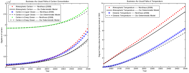
Figure 7: Business-as-usual paths for calibration

Appendix D—Calibration of the Stochastic Climate Tipping Process

We first calibrate the probability of triggering the tipping point event. Given Equation 15, we need to calibrate $\lambda$, the hazard rate parameter, and $\underline{T_{\mathrm{AT}}}$, the lower bound of atmospheric temperature (e.g., today’s temperature level), for which $p_{1,1,0}=0$. Ideally, climate scientists would specify a value for the hazard rate parameter $\lambda$. Unfortunately, no studies exist that would provide specific conditional probabilities of triggering a tipping point event for any given location in the state space. According to Kriegler et al. (2009) there is a substantial lack of knowledge about the underlying physical processes of climate tipping elements. The most reliable source of information is reviews of expert opinion on the cumulative trigger probability at some distant time given some degree of global warming, for example 3 degrees Celsius in 2100 (see Kriegler et al. 2009; Zickfeld et al. 2007; and Lenton 2010). The subjective probability assessments differ significantly among experts, albeit the range of uncertainties about the likelihood of triggering a tipping point being much lower for some climate elements (Kriegler et al. 2009). However, the absence of precise knowledge about the physical system is not essentially a problem for our analysis: decisions today must be based on current beliefs about the climate system and will reflect the imprecise nature of those beliefs. Therefore, we make use of the assessed cumulative trigger probabilities of tipping and infer trigger hazard rates from them. Doing so, we assume tacitly that the subjective expert opinions are the same as those held by the social planner. Lenton (2010) provides for several climate elements the cumulative probability of triggering a tipping point. We choose Lenton (2010) as the source of data because he summarizes the findings from Kriegler et al. (2008) and other expert elicitation studies. Since our interest is in modeling a representative tipping element we use the average of these numbers to approximate the probability of triggering a representative climate tipping element.

The first two rows of Table 15 depict the cumulative probabilities of triggering a climate tipping event until 2100 for different levels of global warming until 2100. We have inferred these numbers from Lenton (2010). These numbers imply, for example, that given a $4$ degrees Celsius increase in global warming in the year 2100, the likelihood of a tipping point event being triggered until 2100 is 50 percent. Our goal is to use these numbers to compute an annual conditional trigger probability. We do this by first specifying the general relationship between a hazard rate $h_{t}$ and the contemporaneous level of global warming above the 2000 temperature in a simple linear form by $h_{t}=\lambda\overset{}{\tilde{T}_{\mathrm{AT},t}}$, where $\lambda$ is a hazard rate parameter and $\tilde{T}_{\mathrm{AT},t}$ is the nominal change in temperature above the year 2000 level ($t$ represents year $t+2000$ here). We then assume that experts in general express their subjective probabilities having in mind that temperature linearly evolves until the specified level at the end of this century.

We then integrate the hazard rate $h_{t}$ up for 100 years and obtain the cumulative hazard $H_{100}.$ The probability of a tipping point having not occurred during this century is then $\exp\left(-H_{100}\right)$. It follows that $P$, the cumulative probability of a tipping point having been triggered until 2100, is $P=1-\exp\left(-H_{100}\right)$. With the former equation we can solve for the hazard rate parameter $\lambda$ :

$$\lambda=-\frac{\log(1-P)}{50\left(\tilde{T}_{\mathrm{AT},100}-\tilde{T}_{\mathrm{AT},0}\right)}.$$ (25)

$\tilde{T}_{\mathrm{AT},100}-\tilde{T}_{\mathrm{AT},0}$	1 °C	2 °C	3 °C	4 °C	5 °C	6 °C
$P$ (cumulative probability until 2100)	12.5%	25%	37.5%	50%	62.5%	75%
$\lambda$ (inferred hazard rate parameter)	0.00267	0.00288	0.00313	0.00347	0.00392	0.00462

Table 15: Cumulative probabilities of triggering a representative tipping element (until 2100) for different levels of global warming and the inferred hazard rate parameter

We use the above expression for the hazard rate parameter and plug in for each column of Table 15 the levels of $\tilde{T}_{\mathrm{AT},100}-\tilde{T}_{\mathrm{AT},0}$ and $P$. We report the computed hazard rate parameter respectively in the bottom row of Table 15. For our previous example of a 4 degrees Celsius increase in global warming and a cumulative trigger probability of 50 percent, our calibration implies a hazard rate parameter of roughly 0.0035, which is approximately the central value in our calibrated range. Practically, $\lambda=0.0035$ implies that, for example, a two-degree increase in temperature (above year 2000) until year 2090 would yield a conditional probability of triggering the tipping point event in the year 2090 of about 0.7 percent. We choose $\lambda=0.0035$ as the default parameter setting for our benchmark case and set up a range for the sensitivity analysis as $\lambda\in[0.0025,0.0045]$. Since we choose not to model any specific tipping element explicitly, we set up the range with respect to how different hazard rate specifications relate to the optimal social cost of carbon. Finally, we set $\underline{T_{\mathrm{AT}}}$ = $1$ degree Celsius, which we calibrate as today’s global warming using a climate emulator (Meinshausen et al. 2011).

Next, we turn to the calibration of $\overline{\mathcal{D}}$, the expected duration of the tipping process. Climate scientists note that tipping elements in the climate system exhibit heterogeneity with respect to their assumed duration of the post-tipping process. According to Lenton et al. (2008) the post-tipping process may last less than ten years or up to several centuries. Table 16 presents the expected transition scale for selection of the most prominent tipping elements from Lenton et al. (2008).

		Arctic			Atlantic	West	West	El Nino
Tipping	Greenland	summer	Amazon	Boreal	thermohaline	Antarctic	African	Southern
Element	ice sheet	sea-ice	rainforest	forests	circulation	ice sheet	monsoon	Oscillation
Expected
transition	>300	10	50	50	100	>300	10	100
scale (years)

Table 16: Duration of expected transition scales for different climate tipping elements

Following the numbers in Table 16 we choose $\overline{\mathcal{D}}=50$ (years) for our benchmark tipping process. In addition, in our sensitivity analyses we also consider $\overline{\mathcal{D}}=5$ (years) as the lower bound, $\overline{\mathcal{D}}=100$ (years), and $\overline{\mathcal{D}}=200$ (years) as the upper bound. As mentioned in the main text, we assume that each of our five stages occurs stochastically and the expected transition time at each stage of the tipping process is $\overline{\mathcal{D}}/4$ years.

In this paper, all of our examples of tipping elements assume that there are three possible tipping damage levels in the long run if $q>0$, and that we do not know the long-run damage level until tipping begins. Since the variance of the long-run tipping damage level is $q\overline{\mathcal{J}}_{\infty}^{2}$, we assume that the values of the three possible tipping damage levels in the long run are $\left(1+\left(j-2\right)\sqrt{1.5q}\right)\overline{\mathcal{J}}_{\infty}$, for $j=1,2,3$, with equal probability. For our benchmark case with $\overline{\mathcal{J}}_{\infty}=5\%$ and $q=0.2$ the three possible long-run damage levels are 2.26 percent, 5 percent, and 7.74 percent, each with 1/3 probability. In the extreme cases of $\overline{\mathcal{J}}_{\infty}=2.5\%$ (or $\overline{\mathcal{J}}_{\infty}=10\%$) and $q=0.4$ in our sensitivity analysis, the three possible long-run damage levels are 0.56 percent, 2.5 percent, and 4.44 percent (or 2.25 percent, 10 percent, and 17.75 percent).

We also assume that the cascading damage linearly increases over the five post-tipping stages. That is, if the level of long-run tipping damage is $\left(1+\left(j-2\right)\sqrt{1.5q}\right)\overline{\mathcal{J}}_{\infty}$, then the damage at the $i$-th post-tipping stage is $\left(1+\left(j-2\right)\sqrt{1.5q}\right)\overline{\mathcal{J}}_{\infty}\cdot i/5$, for $i=1,2,...,5$. Thus, the values of $J_{t}$ are: $\mathcal{J}_{1}=0$ and

$$\mathcal{J}_{3i+j-2}=\frac{i}{5}\left(1+\left(j-2\right)\sqrt{1.5q}\right)\overline{\mathcal{J}}_{\infty},$$ (26)

for $i=1,...,5$ and $j=1,2,3$. When $q=0$, there are only six values of $J_{t}$: $\mathcal{J}_{1}=0$ and $\mathcal{J}_{i+1}=\overline{\mathcal{J}}_{\infty}\cdot i/5$ for $i=1,2,...,5$.

Since we assume that we know the long-run damage level once the tipping event happens and the three possible levels are equally distributed, the probability from the pre-tipping state $\mathcal{J}_{1}$ to $\mathcal{J}_{1+j}$ at time $t$ is $p_{1,1+j,t}=\left(1-p_{1,1,t}\right)/3$ for $j=1,2,3$. Moreover, if the current state is $\mathcal{J}_{3i+j-2}$ with $i<5$, meaning that it is at the $i$-th post-tipping stage, then it could either stay with the probability $\exp\left(-4/\overline{\mathcal{D}}\right)$, or move to state $\mathcal{J}_{3(i+1)+j-2}$ (the $(i+1)$-th post-tipping stage) with the probability $1-\exp\left(-4/\overline{\mathcal{D}}\right)$. Therefore, the Markov chain transition matrix of the state $J_{t}$ at time $t$ is a $16\times 16$ matrix with the following sparsity shape:

$$\left[\begin{array}[]{ccccccc}*&*&*&*\\ &*&&&*\\ &&\ddots&&&\ddots\\ &&&*&&&*\\ &&&&1\\ &&&&&1\\ &&&&&&1\end{array}\right],$$

where a star means one nonzero element. The $(1,1)$ element, $p_{1,1,t}$, is given by (15), the $(1,j)$ element is $p_{1,j,t}=\left(1-p_{1,1,t}\right)/3$ for $j=2,3,4$, the $(i,i)$ element is $p_{i,i,t}=\exp\left(-4/\overline{\mathcal{D}}\right)$, and the $(i,i+3)$ element is $p_{i,i+3,t}=1-p_{i,i,t}$ for $i=2,...,13$. The last three diagonal elements are 1’s, implying irreversibility. When $q=0$, the matrix is reduced to a $6\times 6$ bidiagonal matrix, where the $(1,1)$ element is still given by (15), but the $(i,i)$ element is $p_{i,i,t}=\exp\left(-4/\overline{\mathcal{D}}\right)$, the $(i,i+1)$ element becomes $p_{i,i+1,t}=1-p_{i,i,t}$ for $i=2,3,4,5$, and the $(6,6)$ element is 1.

Appendix E—Value Function Iteration

We summarize the numerical method we used to solve the dynamic programming problems in this study. The value functions for our problems are continuous, and almost everywhere differentiable in the continuous state variables. In each case, we approximate the value function $V(x,\theta)$ using a functional form $\hat{V}(x,\theta;{\bf b})$ with a finite number of parameters, ${\bf b}$. In our model, the state variable $x$ represents the six-dimensional vector $(K,\mathbf{M},\mathbf{T})$ of continuous states, and $\theta$ represents the three-dimensional vector of discrete states, $(\zeta,\chi,J)$, contained in a finite set $\Theta$. The functional form $\hat{V}$ may be a linear combination of polynomials, a rational function, a neural net, or some other parameterization specially designed for the problem. After the functional form is set, we focus on finding the vector of parameters, ${\bf b}$, such that $\hat{V}(x,\theta;{\bf b})$ approximately satisfies the Bellman equation (Bellman, 1957). Numerical dynamic programming with value function iteration can solve the Bellman equation approximately (Judd, 1998).

A general dynamic programming model is based on the Bellman equation:

$$V_{t}(x,\theta)=\max_{a\in{\cal D}(x,\theta,t)}\text{ \ }u_{t}(x,a)+\beta\mathcal{H}_{t}\left(V_{t+1}(x^{+},\theta^{+})\right),$$

$$\text{{\rm\ \ \ \ \ \ \ \ \ \ \ \ \ \ \ \ \ s.t. \ \ }}x^{+}=F(x,\theta,a),$$

$$\text{{\rm\ \ \ \ \ \ \ \ \ \ \ \ \ \ \ \ \ \ \ \ \ \ \ \ }}\theta^{+}=G(x,\theta,\omega),$$

where $V_{t}(x,\theta)$ is the value function at time $t\leq\mathcal{T}$ (the terminal value function $V_{\mathcal{T}}(x,\theta)$ is given), $(x^{+},\theta^{+})$ is the next-stage state, ${\cal D}(x,\theta,t)$ is a feasible set of $a$, $\omega$ is a random variable vector, $F$ and $G$ are the transition laws of $x$ and $\theta$, $\beta$ is a discount factor and $u_{t}(x,a)$ is the utility function, and $\mathcal{H}_{t}$ is a functional operator at time $t$. The following is the algorithm of parametric dynamic programming with value function iteration for finite horizon problems.

Algorithm

1. Numerical Dynamic Programming with Value Function Iteration for Finite Horizon Problems

Initialization.

Choose the approximation nodes, $\mathbb{X}_{t}=\{x_{i,t}:$ $1\leq i\leq m_{t}\}$ for every $t<\mathcal{T}$, and choose a functional form for $\hat{V}(x,\theta;{\bf b})$, where $\theta\in\Theta$. Let $\hat{V}(x,\theta;{\bf b}_{\mathcal{T}})\equiv V_{\mathcal{T}}(x,\theta)$. Then for $t=\mathcal{T}-1,\mathcal{T}-2,\ldots,0$, iterate through steps 1 and 2.

Step

1. Maximization step. Compute

$$v_{i,j}=\max_{a\in{\cal D}(x_{i},\theta_{j},t)}\ u_{t}(x_{i},a)+\beta\mathcal{H}_{t}\left(\hat{V}\left(x^{+},\theta_{j}^{+};{\bf b}_{t+1}\right)\right)$$

$$\text{{\rm\ \ \ \ \ \ \ \ \ \ \ \ \ s.t. \ \ \ }}x^{+}=F(x_{i},\theta_{j},a),$$

$$\text{{\rm\ \ \ \ \ \ \ \ \ \ \ \ \ \ \ \ \ \ \ \ \ \ }}\theta_{j}^{+}=G(x_{i},\theta_{j},\omega),$$

for each $\theta_{j}\in\Theta$, $x_{i}\in\mathbb{X}_{t}$, $1\leq i\leq m_{t}.$

Step

2. Fitting step. Using an appropriate approximation method, compute the ${\bf b}_{t}$ such that $\hat{V}(x,\theta_{j};{\bf b}_{t})$ approximates $(x_{i},v_{i,j})$ data for each $\theta_{j}\in\Theta$.

We considered alternative functional forms for $\hat{V}(x,\theta;{\bf b})$, including ordinary polynomials and polynomials in logs. We were always able to find some parsimonious functional form for approximating the value function. Detailed discussion of numerical dynamic programming methods can be found in Cai (2010), Cai and Judd (2010), Judd (1998), and Rust (2008).

The terminal value function is computed by assuming that after 2600, the system is deterministic, population and productivity growth ends, all emissions are eliminated, and the consumption-output ratio is fixed at 0.78. Consideration of alternatives showed that changes in the terminal value function at 2600 had no significant impact on any results for the 21st century.

Appendix F—Code Test

In order to have confidence in our code, we compared how our code performed on a few cases where we could compute the true solution using another method. The key challenge for any dynamic programming problem, deterministic or stochastic, is the ability to accurately approximate the value function over a large range of possible values. Our tests were to compute solutions to deterministic versions of our models, that is, versions where we eliminate all randomness, by two methods: our dynamic programming code and by optimal control methods. Since the latter can be computed with high accuracy, we can compare those solutions with the results of the dynamic programming algorithm. For example, among the three benchmark cases, the approximation domains for the stochastic growth and climate tipping benchmark case are the widest because it has the largest volatility, and then we use the highest degree polynomials for approximation. We performed three tests, each using the same approximation domains and polynomial degrees as used in one of the three benchmark cases. Table 17 shows the relative $\mathcal{L}^{1}$ errors over the first one hundred years of three of the endogenous state variables ($K$, $M_{\mathrm{AT}}$, $T_{\mathrm{AT}}$), two control variables ($C$, $\mu$), and the social cost of carbon. It also shows the relative error in the initial year for the control variables and the social cost of carbon. Table 17 shows that all the relative errors were small.

Variable	Test case (deterministic) with		Test case (deterministic) with		Test case (deterministic) with
	approximation degrees and		approximation degrees and		approximation degrees and
	domains of the stochastic		domains of the stochastic		domains of the stochastic growth
	growth benchmark case		climate benchmark case		and climate benchmark case
	first 100 years	initial year	first 100 years	initial year	first 100 years	initial year
$K$	$5.5(-3)$	—	$2.1(-4)$	—	$4.0(-3)$	—
$M_{\mathrm{AT}}$	$1.5(-4)$	—	$1.3(-5)$	—	$1.1(-4)$	—
$T_{\mathrm{AT}}$	$8.7(-5)$	—	$2.5(-5)$	—	$8.3(-5)$	—
$C$	$2.0(-3)$	$4.6(-5)$	$2.4(-5)$	$2.6(-5)$	$1.6(-3)$	$4.0(-5)$
$\mu$	$2.4(-3)$	$1.3(-4)$	$4.4(-4)$	$1.7(-4)$	$2.0(-3)$	$1.3(-4)$
$\Gamma$	$9.2(-3)$	$5.4(-3)$	$4.1(-3)$	$7.2(-4)$	$1.0(-2)$	$6.2(-3)$

Table 17: Relative errors for the solution of the deterministic case obtained by our numerical dynamic programming algorithm with approximation domains and polynomial degrees used by the three benchmark cases. Note—$a(-n)$ means $a\times 10^{-n}$

Appendix G—Dynamics of the Economic System in the Stochastic Growth Benchmark Case

Figure 8 shows the dynamics of gross world output ($\mathcal{Y}_{t}$), total capital ($K_{t}$), and per capita consumption growth rate. Both gross world output and the total capital stock grow exponentially, which is not surprising since productivity grows exponentially. The uncertainty of both is substantial; for example the 10 percent and 90 percent quantiles of the capital stock in 2100 are $270 trillion and $1,500 trillion respectively. The growth of per capita consumption in Figure 8C ranges from $-4.4\%$ to $7.1\%$. The mean and median of the dynamic stochastic equilibrium paths are close to the deterministic solution, but the variation around that path is very large.

The wide range of possible outcomes for the total capital stock displayed in Figure 8B implied that our approximation of the value function had to be defined over an even larger range. The blue broken lines in Figure 8B represent, for each time $t$, the minimum and maximum level of the capital stock (on $\log_{10}$ scale) over which the value function is computed. The ratio of maximum to minimum capital stock exceeded 175 in 2100, and continues to grow thereafter. If we had used significantly smaller ranges then the Bellman equation for states close to the maximum or minimum capital stock would try to evaluate the value function beyond the domain on which it is approximated. These ranges are the natural outcome of the productivity process. The large range for capital creates difficulties for the simpler approximation methods, such as orthogonal polynomials, but nonlinear changes in variables allowed us to find suitable function forms for approximating the value function.

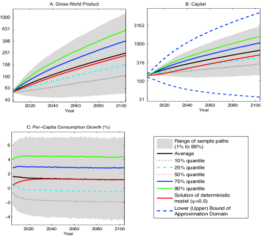
Figure 8: Simulation results of the stochastic growth benchmark—Economics

References

- [1] Ackerman, F., E.A. Stanton, and R. Bueno (2013). Epstein–Zin utility in DICE: is risk aversion irrelevant to climate policy? Environ Resource Econ 56, 73–84.
- [2] Bansal, R., D. Kiku, and A. Yaron (2012). An empirical evaluation of the long-run risks model for asset prices. Critical Finance Review, Issue 1, 183–221.
- [3] Bansal, R., and A. Yaron (2004). Risks for the long run: A potential resolution of asset pricing puzzles. The Journal of Finance, 59(4), 1481–509.
- [4] Bansal, R., and M. Ochoa (2011). Welfare costs of long-run temperature shifts, Duke University Working Paper.
- [5] Barrage, L. (2014). Sensitivity analysis for Golosov, Hassler, Krusell, and Tsyvinski (2014): ‘Optimal taxes on fossil fuel in general equilibrium’ supplemental material, Econometrica, 82(1): 41-88.
- [6] Barro, R.J. (2009). Rare disasters, asset prices, and welfare costs. American Economic Review, 99(1): 243–264.
- [7] Beeler, J., and J.Y. Campbell (2011). The long-run risks model and aggregate asset prices: an empirical assessment. Critical Finance Review 1(1): 141–182.
- [8] Bellman, R. (1957). Dynamic Programming. Princeton University Press.
- [9] Brock, W.A., and D. Starrett (2003). Managing systems with non-convex positive feedback. Environmental and Resource Economics 26 (4): 575–602.
- [10] Cai, Y. (2010). Dynamic Programming and Its Application in Economics and Finance. PhD thesis, Stanford University.
- [11] Cai, Y., and K.L. Judd (2010). Stable and efficient computational methods for dynamic programming. Journal of the European Economic Association, 8(2-3): 626–634.
- [12] Cai, Y., K.L. Judd, and T.S. Lontzek (2012a). Open science is necessary. Nature Climate Change, 2(5): 299.
- [13] Cai, Y., K.L. Judd, and T.S. Lontzek (2012b). Continuous-time methods for integrated assessment models. NBER working paper 18365.
- [14] Cai, Y., K.L. Judd, G. Thain, and S. Wright (2015). Solving dynamic programming problems on computational grid. Computational Economics, 45(2): 261–284.
- [15] Campbell, J.Y., and J.H. Cochrane (1999). By force of habit: a consumption-based explanation of aggregate stock market behavior. Journal of Political Economy 107, 205–251.
- [16] Epstein, L.G., and S.E. Zin (1989). Substitution, risk aversion, and the temporal behavior of consumption and asset returns: a theoretical framework. Econometrica, 57(4), 937–969.
- [17] Golosov, M., J. Hassler, P. Krusell, and A. Tsyvinski (2014). Optimal taxes on fossil fuel in general equilibrium. Econometrica, 82(1): 41–88.
- [18] Hope, C. (2011). The PAGE09 integrated assessment model: a technical description. Cambridge Judge Business School Working Paper 4/2011. Accessed June 23, 2014: http://www.jbs.cam.ac.uk/fileadmin/user_upload/research/workingpapers/wp1104.pdf
- [19] IWG (2010). Social Cost of Carbon for Regulatory Impact Analysis under Executive Order 12866. United States Government. http://www.whitehouse.gov/sites/default/files/omb/inforeg/for-agencies/Social-Cost-of-Carbon-for-RIA.pdf
- [20] IPCC (2013). Summary for Policymakers. In: Climate Change 2013: The Physical Science Basis. Contribution of Working Group I to the Fifth Assessment Report of the Intergovernmental Panel on Climate Change. Cambridge University Press, Cambridge, United Kingdom and New York, NY, USA.
- [21] IPCC (2014). Climate Change 2014: Impacts, Adaptation, and Vulnerability. Part A: Global and Sectoral Aspects. Contribution of Working Group II to the Fifth Assessment Report of the Intergovernmental Panel on Climate Change. Cambridge University Press, Cambridge, United Kingdom and New York, NY, USA.
- [22] Jensen, S., and Traeger, C. (2014). Optimal climate change mitigation under long-term growth uncertainty: stochastic integrated assessment and analytic findings. European Economic Review 69, 104–125.
- [23] Joughin, I., B.E. Smith, and B. Medley (2014). Marine ice sheet collapse potentially under way for the Thwaites Glacier Basin, West Antarctica. Science 344, 735–738.
- [24] Judd, K.L. (1998). Numerical Methods in Economics. The MIT Press.
- [25] Keller, K., B. Bolker, and D.F. Bradford (2004). Uncertain climate thresholds and optimal economic growth. Journal of Environmental Economics and Management 48, 723–741.
- [26] Kelly, D.L., and C.D. Kolstad (1999). Bayesian learning, growth, and pollution. Journal of Economic Dynamics and Control 23, 491–518.
- [27] Kopits, E., A. Marten, and A. Wolverton (2014). Incorporating ’catastrophic’ climate change into policy analysis. Climate Policy 14(5): 637–664.
- [28] Kreps, D.M., and E.L. Porteus (1978). Temporal resolution of uncertainty and dynamic choice theory. Econometrica 46(1): 185–200.
- [29] Kriegler, E., J.W. Hall, H. Held, R. Dawson, and H.J. Schellnhuber (2009). Imprecise probability assessment of tipping points in the climate system. PNAS 106(13): 5041–5046.
- [30] Lemoine, D.M., and C. Traeger (2014). Watch Your Step: Optimal Policy in a Tipping Climate. American Economic Journal: Economic Policy, 6(1), 137–166.
- [31] Lenton, T.M. (2010). Earth System Tipping Points. Working Paper. http://yosemite.epa.gov/ee/epa/eerm.nsf/vwAN/EE-0564-112.pdf/$file/EE-0564-112.pdf
- [32] Lenton, T.M., and J-C. Ciscar (2013). Integrating tipping points into climate impact assessments. Climatic Change 117, 585–597.
- [33] Lenton, T.M., H. Held, E. Kriegler, J. Hall, W. Lucht, S. Rahmstorf, and H.J. Schellnhuber (2008). Tipping elements in the Earth’s climate system. PNAS 105, 1786–1793.
- [34] Lucas, R. E. (1978). Asset pricing in an exchange economy. Econometrica 46, 1429–1445.
- [35] Manne, A., and R. Richels (2005). MERGE: an integrated assessment model for global climate change. Energy and Environment (175–189) edited by. Loulou, R., Waaub, J-P. and Zaccour, G.
- [36] Mastrandrea, M.D., and S.H. Schneider (2001). Integrated assessment of abrupt climatic changes. Climate Policy 1, 433–449.
- [37] Meinshausen, M., S.C.B. Raper, and T.M.L. Wigley (2011). Emulating coupled atmosphere-ocean and carbon cycle models with a simpler model, MAGICC6: Part I – Model Description and Calibration. Atmospheric Chemistry and Physics 11, 1417–1456.
- [38] Nordhaus, W.D. (2007). A review of the Stern Review on the economics of climate change. Journal of Economic Literature 45, 686–702.
- [39] Nordhaus, W.D. (2008). A Question of Balance: Weighing the Options on Global Warming Policies. Yale University Press.
- [40] Nordhaus, W.D. (2012). An Analysis of the Dismal Theorem. Cowles Foundation for Research in Economics. Yale University, 2009. 20
- [41] Nordhaus, W.D., and Z. Yang (1996). A regional dynamic general-equilibrium model of alternative climate-change strategies. American Economic Review, 86, 741–765.
- [42] National Research Council (2013). Abrupt Impacts of Climate Change: Anticipating Surprises. Washington, DC: The National Academies Press, 2013.
- [43] Oberkampf, W.L., and C.J. Roy (2010). Verification and Validation in Scientific Computing. Cambridge University Press.
- [44] Pindyck, R.S. (2013). Climate change policy: what do the models tell us? Journal of Economic Literature, 51(3): 860–872.
- [45] Pindyck, R.S., and N. Wang (2013). The economic and policy consequences of catastrophes. American Economic Journal: Economic Policy, 5(4): 306–339.
- [46] Polasky, S., A. de Zeeuw, and F. Wagener (2011). Optimal management with potential regime shifts. Journal of Environmental Economics and Management, 62(2): 229–240.
- [47] Revesz, R.L., K. Arrow, L.H. Goulder, P.H. Howard, R.E. Kopp, M.A. Livermore, M. Oppenheimer, and T. Sterner (2014). Improve economic models of climate change: costs of carbon emissions are being underestimated, but current estimates are still valuable for setting mitigation policy. Nature 508, 173–175.
- [48] Rust, J. (2008). Dynamic Programming. In: Durlauf, S.N., Blume L.E. (Eds.), New Palgrave Dictionary of Economics. Palgrave Macmillan, second edition.
- [49] Schneider, S.H. (1989). Global warming: scientific reality of political hype. In: Global Warming: Hearings Before the Subcommittee on Energy and Power of the Committee on Energy and Commerce House of Representatives One Hundred First Congress, Serial No. 101-31, pp. 53–66.
- [50] Schneider, S.H., and S.L. Thompson (1981). Atmospheric CO2 and Climate: Importance of the Transient Response. Journal of Geophysical Research, 86(C4), 3135–3147.
- [51] Smith, J.B., S.H. Schneider, M. Oppenheimer, G.W. Yohe, W. Hare, M.D. Mastrandrea, A. Patwardhan, I. Burton, J. Corfee-Morlot, C.H.D. Magadza, H.M. Füssel, A.B. Pittock, A. Rahman, A. Suarez, and J.P. Van Ypersele. (2009). Assessing dangerous climate change through an update of the Intergovernmental Panel on Climate Change (IPCC) ’Reasons for concern’. PNAS 106(11), 4133–4137.
- [52] Stern, N. H. (2007). The economics of climate change: the Stern Review. Cambridge, UK: Cambridge University Press.
- [53] Tauchen, G. (1986). Finite state Markov-chain approximations to univariate and vector autoregressions, Economic Letters, 20, 177–181.
- [54] Vissing-Jørgensen, A. (2002). Limited asset market participation and the inter-temporal elasticity of substitution. Journal of Political Economy 110, 825–853.
- [55] Vissing-Jørgensen, A., and O.P. Attanasio (2003). Stock-market participation, inter-temporal substitution, and risk-aversion, The American Economic Review 93(2): 383–391.
- [56] Weitzman, M.L. (2009). On modeling and interpreting the economics of catastrophic climate change. Review of Economics and Statistics, 91, 1–19.
- [57] Weitzman, M.L., (2012). GHG targets as insurance against catastrophic climate damages. Journal of Public Economic Theory 14(2): 221–244.
- [58] Yohe, G.W., R.D. Lasco, Q.K. Ahmad, N.W. Arnell, S.J. Cohen, C. Hope, A.C. Janetos and R.T. Perez (2007). Perspectives on climate change and sustainability. Climate Change 2007: Impacts, Adaptation and Vulnerability. Contribution of Working Group II to the Fourth Assessment Report of the Intergovernmental Panel on Climate Change, M.L. Parry, O.F. Canziani, J.P. Palutikof, P.J. van der Linden and C.E. Hanson, Eds., Cambridge University Press, Cambridge, UK, 811-841.
- [59] Zickfeld K., A. Levermann, M.G. Morgan, T. Kuhlbrodt, S. Rahmstorf, and D.W. Keith (2007). Expert judgements on the response of the Atlantic meridional overturning circulation to climate change. Climate Change 82, 235–265.
- [60]