Existence and bifurcation of solutions for a double coupled system of Schrödinger equations

Abstract

Consider the following system of double coupled Schrödinger equations arising from Bose-Einstein condensates etc.,

$$\left\{\begin{array}[]{l}-\Delta u+u=\mu_{1}u^{3}+\beta uv^{2}-\kappa v,\\ -\Delta v+v=\mu_{2}v^{3}+\beta u^{2}v-\kappa u,\\ u\neq 0,v\neq 0\ \hbox{and}\ u,v\in H^{1}(\mathbb{R}^{N}),\end{array}\right.$$

where $\mu_{1},\mu_{2}$ are positive and fixed; $\kappa$ and $\beta$ are linear and nonlinear coupling parameters respectively. We first use critical point theory and Liouville type theorem to prove some existence and nonexistence results on the positive solutions of this system. Then using the positive and non-degenerate solution of the scalar equation $-\Delta\omega+\omega=\omega^{3}$, $\omega\in H_{r}^{1}(\mathbb{R}^{N})$, we construct a synchronized solution branch to prove that for $\beta$ in certain range and fixed, there exist a series of bifurcations in product space $\mathbb{R}\times H^{1}_{r}(\mathbb{R}^{N})\times H^{1}_{r}(\mathbb{R}^{N})$ with parameter $\kappa$.

35B32, 35B38, 35J50, 58C40, 58E07

Citation:​​​​

TIAN R S, ZHANG Z T. Science China: Mathematics title. Sci China Math, 2014, 57, doi: 10.1007/s11425-000-0000-0

1 Introduction

In this paper, we study the following elliptic system

$$\left\{\begin{array}[]{l}-\Delta u+u=\mu_{1}u^{3}+\beta uv^{2}-\kappa v,\\ -\Delta v+v=\mu_{2}v^{3}+\beta u^{2}v-\kappa u,\\ u\neq 0,v\neq 0\ \hbox{and}\ u,v\in H^{1}(\mathbb{R}^{N}),\end{array}\right.$$ (1.1)

where $\kappa,\beta$ are coupling parameters, $\mu_{2}\geq\mu_{1}>0$ are constants, $N=2,3$. System (1.1) describes the standing wave solutions of coupled Schrödinger equations, which have wide applications in physics, such as nonlinear optics and Bose-Einstein condensates. See [12, 20, 24] and references therein for more details.

In the presence of only one coupling parameter, either $\kappa$ or $\beta$, extensive research has been done regarding the existence, multiplicity and asymptotic behavior of nontrivial solutions to (1.1). The obtained results are very interesting and important, we refer to [1]-[3], [6]-[11], [14]-[18],[21]-[22],[25]-[29] and references therein. If $\kappa\beta\neq 0$, i.e., the linearly coupling terms and nonlinearly coupling terms both exist, to our best knowledge, analogous research is almost empty. The current paper is devoted to this double coupled case. The main goal of this paper is two-fold:

1. determine regions in $\kappa\beta$-plane for existence and nonexistence of positive solutions to (1.1);

2. refine the existence results in the case $\mu_{1}=\mu_{2}$ by using bifurcation theory, and get more quantitative descriptions for these solutions.

We begin with some notations. Denote by $|\cdot|_{p}$ the usual norm of the space $L^{p}(\mathbb{R}^{N})$ and $\mathcal{H}=H^{1}(\mathbb{R}^{N})\times H^{1}(\mathbb{R}^{N})$, where

$$H^{1}(\mathbb{R}^{N})=\{u\in L^{2}(\mathbb{R}^{N})|\nabla u\in L^{2}(\mathbb{R}^{N})\}$$

is the Hilbert space equipped with the following inner product and induced norm

$$\langle u,v\rangle:=\int_{\mathbb{R}^{N}}(\nabla u\nabla v+uv),\hskip 28.45274pt\|u\|:=\sqrt{(\int_{\mathbb{R}^{N}}|\nabla u|^{2}+|u|^{2})}.$$

Accordingly, the inner product and induced norm on $\mathcal{H}$ are given by

$$\langle(u,v),(\xi,\eta)\rangle=\int_{\mathbb{R}^{N}}(\nabla u\nabla\xi+\nabla v\nabla\eta+u\xi+v\eta),\hskip 17.07182pt\|(u,v)\|_{\mathcal{H}}=\sqrt{\|u\|^{2}+\|v\|^{2}},$$

respectively. Let $\mathcal{H}_{r}:=H_{r}^{1}(\mathbb{R}^{N})\times H_{r}^{1}(\mathbb{R}^{N})$, where

$$H_{r}^{1}(\mathbb{R}^{N})=\{u\in H^{1}(\mathbb{R}^{N})~{}|~{}u~{}\hbox{is radially symmetric}\}.$$

A solution $(u,v)$ of (1.1) is called a positive solution if $u>0,v>0$ in $\mathbb{R}^{N}$. A solution of (1.1) is called a ground state solution if it minimizes the energy functional $I_{\kappa,\beta}:\mathcal{H}\rightarrow\mathbb{R}$,

$$I_{\kappa,\beta}(u,v)=\frac{1}{2}(\|u\|^{2}+\|v\|^{2})+\kappa\int_{\mathbb{R}^{N}}uv-\frac{1}{4}\int_{\mathbb{R}^{N}}(\mu_{1}u^{4}+\mu_{2}v^{4})-\frac{\beta}{2}\int_{\mathbb{R}^{N}}u^{2}v^{2}$$ (1.2)

on the associated Nehari manifold

$$\mathcal{M} =\{(u,v)\in\mathcal{H}~{}|~{}\langle I_{\kappa,\beta}^{\prime}(u,v),(u,v)\rangle=0,u\neq 0,v\neq 0\}$$

$$=\left\{(u,v)\in\mathcal{H}~{}\bigg{|}~{}\|u\|^{2}+\|v\|^{2}+2\kappa\int_{\mathbb{R}^{N}}uv=\int_{\mathbb{R}^{N}}(\mu_{1}u^{4}+\mu_{2}v^{4}+2\beta u^{2}v^{2}),u\neq 0,v\neq 0\right\}.$$

An important observation will be used later is that the ground state solution has positive energy if $-1<\kappa<0$. See Lemma 2.3.

Our first result concerns the existence and nonexistence of positive solutions to (1.1).

Theorem 1.1.

System (1.1) has

1. no positive solution, if $\kappa<-1$ and $\beta\geq\bar{\beta}:=-(\mu_{1}^{2}\mu_{2})^{1/3}$ or $\kappa=-1$ and $\beta>0$;

2. one positive ground state solution if $\kappa\in(-1,0)$ and $\beta>0$.

In particular, if $\mu_{1}=\mu_{2}$ (without loss of generality, assume $\mu_{1}=\mu_{2}=1$), (1.1) has at least one positive solution in $\{(\kappa,\beta)~{}|~{}-1<\kappa\leq 0,\beta\in\mathbb{R}\}\cup\{(\kappa,\beta)~{}|~{}\kappa>0,\beta>-1\}$.

The existence regions and nonexistence regions for positive solutions of (1.1) in $\beta d$-plane are illustrated by Figure 1 and Figure 2 for asymmetric case and symmetric case respectively.

Figure 1: Existence and nonexistence of positive solutions when $\mu_{1}\neq\mu_{2}$

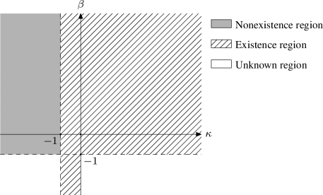
Figure 2: Existence and nonexistence of positive solutions when $\mu_{1}=\mu_{2}=1$,($\bar{\beta}=-1$)

Remark 1.2.

In the case $\kappa=0$ and $\mu_{1}<\mu_{2}$, Bartsch and Wang [6] proved that (1.1) has no positive solution if $\beta\in[\mu_{1},\mu_{2}]$. We can see from Theorem 1.1 (ii) that this nonexistence interval of $\beta$ vanishes when $\kappa$ becomes even sightly less than 0. Also in the case $\kappa=0$, if $\beta\notin[\mu_{1},\mu_{2}]$, it is shown in [5] that (1.1) has at at least one positive solution in $\mathcal{H}_{r}$. This result is extended by Theorem 1.1 (ii) to $-1<\kappa<0$ with the symmetric assumption $\mu_{1}=\mu_{2}$.

We call a solution $(u,v)$ an opposite sign solution if $u>0,v<0$ or $u<0,v>0$ in $\mathbb{R}^{N}$. It can be easily seen that system (1.1) is invariant under the following transformation,

$$\sigma:\mathbb{R}\times\mathbb{R}\times\mathcal{H}\rightarrow\mathbb{R}\times\mathbb{R}\times\mathcal{H},\ \ \ \ \sigma(\kappa,\beta,u,v)=(-\kappa,\beta,u,-v).$$ (1.3)

Using this $\sigma$-invariance of system (1.1), we immediately obtain a corollary of Theorem 1.1 as follows.

Corollary 1.3.

System (1.1) has

1. no opposite sign solution, if $\kappa>1$ and $\beta\geq\bar{\beta}:=-(\mu_{1}^{2}\mu_{2})^{1/3}$ or $\kappa=1$ and $\beta>0$;

2. one opposite sign ground state solution if $\kappa\in(0,1)$ and $\beta>0$.

In particular, if $\mu_{1}=\mu_{2}=1$, (1.1) has at least one pair of opposite sign solutions $(u,v)$ and $(-u,-v)$ in $\{(\kappa,\beta)~{}|~{}0\leq\kappa<1,\beta\in\mathbb{R}\}\cup\{(\kappa,\beta)~{}|~{}\kappa<0,\beta>-1\}$.

The symmetric assumption $\mu_{1}=\mu_{2}$ does not only provide better existence results, but gives rise to two synchronized solution branches as well. More precisely, we assume without loss of generality $\mu_{1}=\mu_{2}=1$, system (1.1) becomes

$$\left\{\begin{array}[]{l}-\Delta u+u+\kappa v=u^{3}+\beta uv^{2},\\ -\Delta v+v+\kappa u=v^{3}+\beta u^{2}v,\\ u\neq 0,v\neq 0\ \hbox{and}\ u,v\in H^{1}(\mathbb{R}^{N}).\end{array}\right.$$ (1.4)

Let $\omega$ be the non-degenerate positive solution of the scalar equation

$$-\Delta\omega+\omega=\omega^{3},\hskip 28.45274pt\omega>0,\hskip 14.22636pt\omega\in H_{r}^{1}(\mathbb{R}^{N}).$$ (1.5)

Then system (1.4) has solutions with two linearly dependent components, $u(x)=a_{1}\omega(bx)$ and $v(x)=a_{2}\omega(bx)$. Substituting this special solution in (1.4) and using the nondegeneracy of $\omega$, we get an algebraic system,

$$\left\{\begin{array}[]{l}a_{1}+\kappa a_{2}=a_{1}b^{2},\\ a_{2}+\kappa a_{1}=a_{2}b^{2},\\ a_{1}^{2}+\beta a_{2}^{2}=b^{2},\\ a_{2}^{2}+\beta a_{1}^{2}=b^{2}.\end{array}\right.$$

By solving this system, we obtain two synchronized solution branches in $\mathbb{R}\times\mathbb{R}\times\mathcal{H}_{r}$,

$$\mathcal{T}_{\omega}^{+}=\left\{\left(\kappa,\beta,\sqrt{\frac{1+\kappa}{1+\beta}}\omega(\sqrt{1+\kappa}x),\sqrt{\frac{1+\kappa}{1+\beta}}\omega(\sqrt{1+\kappa}x)\right)\bigg{|}\beta>-1,\kappa>-1\right\},$$

$$\mathcal{T}_{\omega}^{-}=\left\{\left(\kappa,\beta,\sqrt{\frac{1-\kappa}{1+\beta}}\omega(\sqrt{1-\kappa}x),-\sqrt{\frac{1-\kappa}{1+\beta}}\omega(\sqrt{1-\kappa}x)\right)\bigg{|}\beta>-1,\kappa<1\right\}.$$

Clearly, $\mathcal{T}_{\omega}^{+}$ is a positive solution branch and $\mathcal{T}_{\omega}^{-}$ is an opposite sign solution branch. We will be focusing on bifurcations with respect to $\mathcal{T}_{\omega}^{+}$, then the bifurcation results with respect to $\mathcal{T}_{\omega}^{-}$ will follow immediately by taking advantage of the $\sigma$-invariance of (1.4).

We use $\mathcal{T}_{\omega}^{+}|_{\kappa}$ (respectively $\mathcal{T}_{\omega}^{+}|_{\beta}$) to denote solution branch with fixed $\kappa$ (respectively with fixed $\beta$) and parameterized in $\beta$ (respectively parameterized in $\kappa$). Clearly, $\mathcal{T}_{\omega}^{+}|_{\kappa},\mathcal{T}_{\omega}^{+}|_{\beta}\subset\mathbb{R}\times\mathcal{H}_{r}$.

We call $(\beta_{0},u_{\beta_{0}},v_{\beta_{0}})\in\mathcal{T}_{\omega}^{+}|_{\kappa}$ a bifurcation point if there exist a sequence $(\beta_{j},u_{j},v_{j})\in\mathbb{R}\times\mathcal{H}_{r}\backslash\mathcal{T}_{\omega}^{+}|_{\kappa}$ of solutions of (1.4) such that $(\beta_{j},u_{j},v_{j})\rightarrow(\beta_{0},u_{\beta_{0}},v_{\beta_{0}})$ as $j\rightarrow\infty$. The parameter value $\beta_{0}$ is called a parameter bifurcation point. Similarly, we call $(\kappa_{0},u_{\kappa_{0}},v_{\kappa_{0}})\in\mathcal{T}_{\omega}^{+}|_{\kappa}$ a bifurcation point if there exist a sequence $(\kappa_{j},u_{j},v_{j})\in\mathbb{R}\times\mathcal{H}_{r}\backslash\mathcal{T}_{\omega}^{+}|_{\beta}$ of solutions of (1.4) such that $(\kappa_{j},u_{j},v_{j})\rightarrow(\kappa_{0},u_{\kappa_{0}},v_{\kappa_{0}})$ as $j\rightarrow\infty$. The parameter value $\kappa_{0}$ is also called a parameter bifurcation point.

Denote the set of all nontrivial solutions by

$$\mathcal{S}:=\{(\kappa,\beta,u,v)\in\mathbb{R}\times\mathbb{R}\times\mathcal{H}_{r}\backslash\mathcal{T}_{\omega}^{+}|\ (\kappa,\beta,u,v)\ \hbox{solves \eqref{equ:symmetric}}\}.$$

Also denote the restriction of $\mathcal{S}$ with fixed $\kappa$ by $\mathcal{S}^{\kappa}$, and with fixed $\beta$ by $\mathcal{S}^{\beta}$ respectively. We call $\beta_{0}$ (respectively $\kappa_{0}$) a global bifurcation parameter if

1. there is a connected set of solutions of (1.4) bifurcates from $\mathcal{T}_{\omega}^{+}|_{\kappa}$ at $(\beta_{0},u_{\beta_{0}},v_{\beta_{0}})$ (respectively from $\mathcal{T}_{\omega}^{+}|_{\beta}$ at $(\kappa_{0},u_{\kappa_{0}},v_{\kappa_{0}})$) that is either unbounded in $\mathcal{S}^{\kappa}$ (respectively $\mathcal{S}^{\beta}$), or

2. intersect with $\mathcal{T}_{\omega}^{+}|_{\kappa}$ at a point other than $(\beta_{0},u_{\beta_{0}},v_{\beta_{0}})$ (respectively with $\mathcal{T}_{\omega}^{+}|_{\beta}$ at a point other than $(\kappa_{0},u_{\kappa_{0}},v_{\kappa_{0}}))$.

These two cases are well known as Rabinowitz’s global bifurcation alternatives.

When $\kappa=0$, Bartsch, Dancer and Wang [5] proved the existence of infinitely many bifurcation points with respect to $\mathcal{T}_{\omega}^{+}|_{\kappa=0}$, and also gave descriptions for global bifurcation branches in radial spaces. Similar results were also established in [27, 28] for indefinite systems and $\mu_{1},\mu_{2}\in\mathbb{R}$. Recently, Bartsch [4] considered a system with multiple components and established corresponding bifurcation results. Note that, without the linearly coupling terms, the existence of a synchronized solution branch does not require symmetric assumption $\mu_{1}=\mu_{2}$. On the other hand, when $\beta=0$ and $\kappa\neq 0$, system (1.1) is linearly coupled. Ambrosetti, Ruiz and Cerami [1] gave descriptions on the ground state solution of this type system in the cases $\kappa$ close to $0$ and $-1$. In an unpublished manuscript by E. Abreu and Z.-Q. Wang, the local bifurcation with respect to $\mathcal{T}_{\omega}^{+}|_{\beta=0}$ and at certain $\kappa\in(-1,0)$ was studied.

In the current paper, we shall study the bifurcation phenomena of system (1.4) in the case $\kappa\neq 0$ and $\beta\neq 0$.

Theorem 1.4.

For any fixed $\beta\in(-1,0]$, system (1.4) has finitely many bifurcation points with respect to $\mathcal{T}_{\omega}^{+}|_{\beta}$, where the bifurcation parameter $\kappa\in(-1,\infty)$. Moreover,

1. the number of bifurcations and the $\mathcal{H}$-norm of bifurcating solutions on $\mathcal{T}_{\omega}^{+}|_{\beta}$ both approach infinity as $\beta\rightarrow-1^{+}$;

2. for each bifurcation point $(\kappa_{l},u_{\kappa_{l}},v_{\kappa_{l}})\in\mathcal{T}_{\omega}^{+}|_{\beta}$, $l\geq 1$, there is a global bifurcation branch $\mathcal{S}^{\beta}_{l}\subset\mathbb{R}\times\mathcal{H}_{r}$. If $(\kappa,u,v)\in\mathcal{S}^{\beta}_{l}$ with $-1<\kappa\leq 0$, then $u>0$ and $v>0$.

Remark 1.5.

The positivity of bifurcation solutions is first proved for a modified system (4.1), which has the same bifurcations as system (1.4).

Using Theorem 1.4 and the $\sigma$-invariance of system (1.4), we obtain the following corollary.

Corollary 1.6.

For any fixed $\beta\in(-1,0]$, system (1.4) has finitely many local bifurcations with respect to $\mathcal{T}_{\omega}^{-}|_{\beta}$, where the bifurcation parameter $\kappa\in(-\infty,1)$. Moreover,

1. the number of bifurcations and the $\mathcal{H}$-norm of bifurcating solutions on $\mathcal{T}_{\omega}^{-}|_{\beta}$ both approach infinity as $\beta\rightarrow 1^{-}$;

2. for each bifurcation point $(\kappa_{l},u_{\kappa_{l}},v_{\kappa_{l}})\in\mathcal{T}_{\omega}^{-}|_{\beta}$, $l\geq 1$, there is a global bifurcation branch $\mathcal{S}_{l}^{\beta}\subset\mathbb{R}\times\mathcal{H}_{r}$. If $(\kappa,u,v)\in\mathcal{S}^{\beta}_{l}$ with $0\leq\kappa<1$, then either $u>0$ and $v<0$, or $u<0$ and $v>0$.

This paper is organized as follows. In Section 2, we study the existence and nonexistence of positive solutions of system (1.1). Theorem 1.1 will be established through a few lemmas. In Section 3, we find local bifurcations with respect to $\mathcal{T}_{\omega}^{+}|_{\beta}$. Moreover, we also give the number of bifurcations and some estimates for the $\mathcal{H}$ norm of bifurcation solutions as $\beta\rightarrow-1^{+}$. In Section 4, we show the positivity of bifurcation solutions in a certain range for the coupling parameters. Finally, Theorem 1.4 is proved by combing the results of Section 3 and Section 4.

2 Existence and nonexistence of positive solutions

In this section, we study the existence and nonexistence of positive solutions to (1.1) and (1.4) in terms of $\kappa$ and $\beta$. Lemma 2.1 and Lemma 2.3 hold for general system (1.1), therefore they also hold in the special case (1.4). Lemma 2.6 is only proved for the symmetric system (1.4).

Lemma 2.1.

System (1.1) has no positive solution, if

$\kappa<-1$ and $\beta\geq-(\mu_{1}^{2}\mu_{2})^{1/3}$, or $\kappa=-1$ and $\beta>0$.

Proof 2.2.

Assume for contradiction that $(u,v)$ is a positive solution of (1.1). By the elliptic regularity theory and Sobolev embeddings, $u,v\in C^{2}(\mathbb{R}^{N})$.

Let us consider the case $\kappa\leq-1$, $\beta>0$ first. Add the two equations of (1.1) together and set $U=u+v$, then we get

$$-\Delta U\geq-\Delta U+(1+\kappa)U=\mu_{1}u^{3}+\mu_{2}v^{3}+\beta u^{2}v+\beta uv^{2}\geq CU^{3},$$

where $C=\min\{\mu_{1},\beta/3\}$. Because $U\geq 0$, according to Liouville-type Theorem 2.3 of [11], we must have $U\equiv 0$. This is a contradiction.

Next, consider the case $\kappa<-1$ and $-(\mu_{1}^{2}\mu_{2})^{1/3}\leq\beta\leq 0$. Again, adding the two equations of (1.1) together and setting $U=u+v$, we get

$$-\Delta U+(1+\kappa)U=\mu_{1}u^{3}+\mu_{2}v^{3}+\beta u^{2}v+\beta uv^{2}\geq\mu_{1}^{\frac{1}{3}}(\mu_{1}^{\frac{1}{3}}u-\mu_{2}^{\frac{1}{3}}v)^{2}U.$$

In the case $\kappa<-1$, Liouville-type Theorem 2.3 of [11] implies $U\equiv 0$. This is a contradiction since $U\geq\max\{u,v\}$ and $u,v$ are both positive solutions.

The proof is completed.

The proof of the following existence lemma is modified from [1].

Lemma 2.3.

System (1.1) has a positive ground state solution for $-1<\kappa<0$ and $\beta>0$.

Proof 2.4.

The proof is divided into four steps.

Step 1: $I_{\kappa,\beta}|_{\mathcal{M}}$ has positive lower bound.

Actually, by Sobolev embeddings and Cauchy inequality,

$$\|u\|^{2}+\|v\|^{2}+2\kappa\int_{\mathbb{R}^{N}}uv \geq\|u\|^{2}+\|v\|^{2}+2\kappa\int_{\mathbb{R}^{N}}|u||v|$$

$$\geq(1+\kappa)(\|u\|^{2}+\|v\|^{2})$$

$$\geq\frac{1+\kappa}{2}(\|u\|+\|v\|)^{2},$$

$$\int_{\mathbb{R}^{N}}(\mu_{1}u^{4}+\mu_{2}v^{4}+2\beta u^{2}v^{2}) \leq\int_{\mathbb{R}^{N}}(\mu_{1}u^{4}+\mu_{2}v^{4})+\beta\bigg{(}\int_{\mathbb{R}^{N}}u^{4}+\int_{\mathbb{R}^{N}}v^{4}\bigg{)}$$

$$\leq(\mu_{2}+\beta)(|u|^{4}_{4}+|v|^{4}_{4})$$

$$\leq C(\mu_{2}+\beta)(\|u\|+\|v\|)^{4},$$

where $C>0$ is the embedding constant for $H^{1}(\mathbb{R}^{N})\hookrightarrow L^{4}(\mathbb{R}^{N})$. Thus for any $(u,v)\in\mathcal{M}$, the above estimates yield

$$(\|u\|+\|v\|)^{2}\geq\rho:=\frac{1+\kappa}{2C(\mu_{2}+\beta)}>0.$$ (2.1)

Therefore

$$I_{\kappa,\beta}|_{\mathcal{M}}=\frac{1}{4}\bigg{(}\|u\|^{2}+\|v\|^{2}+2\kappa\int_{\mathbb{R}^{N}}uv\bigg{)}\geq\frac{(1+\kappa)\rho}{8}>0.$$ (2.2)

Step 2: The critical point of $I_{\kappa,\beta}|_{\mathcal{M}}$ is also a critical point of $I_{\kappa,\beta}$.

Assume that $(u_{0},v_{0})$ is a critical point of $I_{\kappa,\beta}|_{\mathcal{M}}$. Denote by $F(u,v)=\langle I_{\kappa,\beta}^{\prime}(u,v),(u,v)\rangle$, then there exists a Lagrange multiplier $\Lambda$ such that

$$I^{\prime}_{\kappa,\beta}(u_{0},v_{0})=\Lambda F^{\prime}(u_{0},v_{0}).$$ (2.3)

Apply both sides to $(u_{0},v_{0})$ and note that $(u_{0},v_{0})\in\mathcal{M}$,

$$0=\langle I^{\prime}_{\kappa,\beta}(u_{0},v_{0}),(u_{0},v_{0})\rangle=\Lambda\langle F^{\prime}(u_{0},v_{0}),(u_{0},v_{0})\rangle.$$ (2.4)

Recall the lower bound of $\mathcal{H}$-norm on $\mathcal{M}$ (2.1), then

$$\langle F^{\prime}(u_{0},v_{0}),(u_{0},v_{0})\rangle =-2(\|u_{0}\|^{2}+\|v_{0}\|^{2})-4\kappa\int_{\mathbb{R}^{N}}u_{0}v_{0}$$

$$\leq-2(1+\kappa)(\|u\|^{2}+\|v\|^{2})$$

$$\leq-(1+\kappa)\rho<0.$$

Combine with (2.4) we get $\Lambda=0$. Now (2.3) gives $I^{\prime}_{\kappa,\beta}(u_{0},v_{0})=0$, i.e. $(u_{0},v_{0})$ is a critical point of $I_{\kappa,\beta}$.

Step 3: $I_{\kappa,\beta}|_{\mathcal{M}}$ satisfies the PS condition.

Since $\kappa\in(-1,0)$, we introduce a new norm on $\mathcal{H}_{r}$:

$$\|(u,v)\|_{1}=\sqrt{\|u\|^{2}+\|v\|^{2}+2\kappa\int_{\mathbb{R}^{N}}uv}.$$

It is easy to verify that

$$(1+\kappa)\|(u,v)\|_{\mathcal{H}}\leq\|(u,v)\|_{1}\leq\sqrt{2}\|(u,v)\|_{\mathcal{H}},$$ (2.5)

i.e., $\|(\cdot,\cdot)\|_{\mathcal{H}}$ and $\|(\cdot,\cdot)\|_{1}$ are equivalent norms on $\mathcal{H}_{r}$. Now let $\{(u_{n},v_{n})\}\subset\mathcal{H}_{r}$ be a PS sequence of $I_{\kappa,\beta}|_{\mathcal{M}}$, i.e., there exists $c\in\mathbb{R}$ such that

$$I_{\kappa,\beta}|_{\mathcal{M}}(u_{n},v_{n})\rightarrow c,\hskip 28.45274ptI^{\prime}_{\kappa,\beta}|_{\mathcal{M}}(u_{n},v_{n})\rightarrow 0\ \hbox{as}\ n\rightarrow\infty.$$

It is easy to see from (2.2) and (2.5) that $\|(u_{n},v_{n})\|_{1}$ is bounded, then there exists a subsequence of $\{(u_{n},v_{n})\}$, still denoted by $\{(u_{n},v_{n})\}$ for simplicity, which weakly converges to $(u,v)$ in $\mathcal{H}_{r}$ with the topology induced by $\|(\cdot,\cdot)\|_{1}$. Using the compact embedding $H^{1}_{r}(\mathbb{R}^{N})\hookrightarrow L^{4}(\mathbb{R}^{N})$, we get $\int_{\mathbb{R}^{N}}u_{n}^{4}\rightarrow\int_{\mathbb{R}^{N}}u^{4}$, $\int_{\mathbb{R}^{N}}v_{n}^{4}\rightarrow\int_{\mathbb{R}^{N}}v^{4}$, and by Hölder inequality,

$$\bigg{|}\int_{\mathbb{R}^{N}}(u_{n}^{2}v_{n}^{2}-u^{2}v^{2})\bigg{|} \leq\int_{\mathbb{R}^{N}}u_{n}^{2}|v_{n}^{2}-v^{2}|+\int_{\mathbb{R}^{N}}v^{2}|u_{n}^{2}-u^{2}|$$

$$\leq|u_{n}|_{4}^{2}\left(\int_{\mathbb{R}^{N}}(v_{n}+v)^{2}(v_{n}-v)^{2}\right)^{\frac{1}{2}}+|v|_{4}^{2}\left(\int_{\mathbb{R}^{N}}(u_{n}+u)^{2}(u_{n}-u)^{2}\right)^{\frac{1}{2}}$$

$$\leq|u_{n}|_{4}^{2}\cdot|v_{n}+v|_{4}\cdot|v_{n}-v|_{4}+|v|_{4}^{2}\cdot|u_{n}+u|_{4}\cdot|u_{n}-u|_{4}$$

$$\rightarrow 0,$$

as $n\rightarrow\infty$. Combine the definition of $\mathcal{M}$ and the above limits, we get $\|(u_{n},v_{n})\|_{1}\rightarrow\|(u,v)\|_{1}$ as $n\rightarrow\infty$. The norm convergence and the weak convergence together imply $(u_{n},v_{n})\rightarrow(u,v)$ strongly in $\mathcal{H}_{r}$. Therefore $I_{\kappa,\beta}|_{\mathcal{M}}$ satisfies the PS condition.

Step 4: $\inf_{\mathcal{M}}I_{\kappa,\beta}$ can be achieved by a positive and radially symmetric function.

Let $\{(u_{n},v_{n})\}$ be a minimizing sequence of $I_{\kappa,\beta}(u,v)|_{\mathcal{M}}$. Then there exist a positive sequence $\{t_{n}\}$ such that $(t_{n}|u_{n}|,t_{n}|v_{n}|)\in\mathcal{M}$. Since $-1<\kappa<0,\beta>0$, there holds

$$t_{n}^{2} =\frac{\|u_{n}\|^{2}+\|v_{n}\|^{2}+2\kappa\int|u_{n}v_{n}|}{\int(\mu_{1}u_{n}^{4}+\mu_{2}v_{n}^{4}+2\beta\int|u_{n}|^{2}|v_{n}|^{2}}\leq\frac{\|u_{n}\|^{2}+\|v_{n}\|^{2}+2\kappa\int u_{n}v_{n}}{\int(\mu_{1}u_{n}^{4}+\mu_{2}v_{n}^{4}+2\beta\int u_{n}^{2}v_{n}^{2}}=1.$$

According to the definition of $I_{\kappa,\beta}|_{\mathcal{M}}$,

$$I_{\kappa,\beta}(t_{n}|u_{n}|,t_{n}|v_{n}|) =\frac{t_{n}^{2}}{4}\left(\|u_{n}\|^{2}+\|v_{n}\|^{2}+2\kappa\int_{\mathbb{R}^{N}}|u_{n}v_{n}|dx\right)$$

$$\leq\frac{1}{4}\left(\|u_{n}\|^{2}+\|v_{n}\|^{2}+2\kappa\int_{\mathbb{R}^{N}}u_{n}v_{n}dx\right)$$

$$=I_{\kappa,\beta}(u_{n},v_{n}).$$

Therefore, we can assume $u_{n}\geq 0,v_{n}\geq 0$.

Denote by $u^{*}_{n},v^{*}_{n}$ the Schwartz symmetrization of $u_{n}$ and $v_{n}$ respectively. Similar to the above arguments, there exists $t_{n}^{*}>0$ such that $(t_{n}^{*}u_{n}^{*},t^{*}_{n}v_{n}^{*})\in\mathcal{M}$. Since

$$\|u_{n}^{*}\|^{2}\leq\|u_{n}\|^{2},\ \ \ \int_{\mathbb{R}^{N}}u_{n}^{*}v_{n}^{*}\geq\int_{\mathbb{R}^{N}}u_{n}v_{n},\ \ \ |u_{n}^{*}|_{4}=|u_{n}|_{4},$$

the same arguments yields $t^{*}_{n}\leq 1$ and $I_{\kappa,\beta}(t^{*}_{n}u^{*}_{n},t^{*}_{n}v_{n}^{*})\leq I_{\kappa,\beta}(u_{n},v_{n})$. Thus we can also assume that the minimizing sequence consists of radial functions. By Step 3, $\inf_{\mathcal{M}}I_{\kappa,\beta}$ has a positive radial minimizer, $(u_{\kappa,\beta},v_{\kappa,\beta})$, which gives a critical point of $I_{\kappa,\beta}|_{\mathcal{M}}$. Then by Step 2, this is also a critical point of $\inf I_{\kappa,\beta}$. By the strong maximum principle we get $u_{\kappa,\beta}>0$ and $v_{\kappa,\beta}>0$, i.e. system (1.1) has a positive ground state solution.

The proof is completed.

Remark 2.5.

In the estimates of $t_{n}$ and $t_{n}^{*}$, the conditions $\kappa\in(-1,0)$ and $\beta>0$ are used, thus the proof of Lemma 2.3 seems hard to be used to find solutions of (1.1) for other values of $\kappa$ or $\beta$.

For the symmetric system (1.4), we can get solutions on a larger region in $\kappa\beta$-plane.

Lemma 2.6.

System (1.4) has at least one positive solutions for every $\kappa>-1$ and $\beta>-1$, and has multiple positive solutions for $-1<\kappa\leq 0$ and $\beta\leq-1$.

Proof 2.7.

If $\kappa>-1$ and $\beta>-1$, then solution branch $\mathcal{T}_{\omega}^{+}$ exists, thus system (1.4) has at least one positive solution.

If $-1<\kappa\leq 0$ and $\beta\leq-1$, positive solution are found by using bifurcation method with respect to $\mathcal{T}_{\omega}^{+}|_{\kappa}$ in parameter $\beta$. Actually, for each $-1<\kappa\leq 0$ fixed, there is a sequence of global bifurcations in radial space $\mathcal{H}_{r}$. Moreover, these global bifurcation branches are unbounded in the negative direction of $\beta$, i.e., the projection of each global bifurcation branch cover the interval $\beta\in(-\infty,-1]$. The proofs are analogous to [5], so the details are omitted.

Remark 2.8.

Due to the presence of parameter $\kappa$, there is no synchronized solution branch if $\mu_{1}\neq\mu_{2}$. Thus, the proof of Lemma 2.6 does not apply to system (1.1) in general.

Proof of Theorem 1.1   It follows directly from Lemma 2.1, 2.3 and 2.6. $\square$

Picture 3 shows the synchronized solution branches $\mathcal{T}_{\omega}^{+}|_{\kappa}$ for three different values of $\kappa$. The bifurcation points on $\mathcal{T}_{\omega}^{+}|_{\kappa}$ coincide with the local bifurcation phenomena demonstrated in [5]. We omit the global bifurcation branches, which are unbounded in the negative direction of $\beta$, to keep the picture clean.

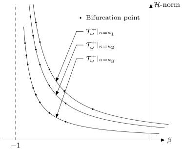
Figure 3: Schematic diagram of $\mathcal{T}_{\omega}^{+}|_{\kappa=\kappa_{i}}$ with $-1<\kappa_{3}<\kappa_{2}<\kappa_{1}=0$.

3 Linearized system and possible parameter bifurcation points

Since the bifurcation phenomena with parameter $\beta$ has been essentially studied in [5], we shall focus on the bifurcations with parameter $\kappa$ in the rest of this paper. Also, we shall work in the radially symmetric space $\mathcal{H}_{r}$ from now on. For simplicity, let $\omega_{\kappa}(x):=\omega(\sqrt{1+\kappa}x)$.

Linearize system (1.4) at $(\kappa,\beta,u,v)\in\mathcal{T}_{\omega}^{+}$, we get

$$-\Delta\left(\begin{array}[]{c}\phi\\ \psi\end{array}\right)+\left(\begin{array}[]{cc}1&\kappa\\ \kappa&1\end{array}\right)\left(\begin{array}[]{c}\phi\\ \psi\end{array}\right) =\left(\begin{array}[]{cc}3u^{2}+\beta v^{2}&2\beta uv\\ 2\beta uv&3v^{2}+\beta u^{2}\end{array}\right)\left(\begin{array}[]{c}\phi\\ \psi\end{array}\right)$$ (3.11)

$$=\frac{(1+\kappa)\omega_{\kappa}^{2}}{1+\beta}\left(\begin{array}[]{cc}3+\beta&2\beta\\ 2\beta&3+\beta\end{array}\right)\left(\begin{array}[]{c}\phi\\ \psi\end{array}\right),$$ (3.16)

where $(\phi,\psi)\in\mathcal{H}_{r}$. Denote the coefficient matrices in (3.11) by,

$$D(\kappa)=\left(\begin{array}[]{cc}1&\kappa\\ \kappa&1\end{array}\right),\hskip 28.45274ptE(\beta)=\left(\begin{array}[]{cc}3+\beta&2\beta\\ 2\beta&3+\beta\end{array}\right).$$

It is easy to see that $(1,1)^{T}$ and $(1,-1)^{T}$ are eigenvectors of $D(\kappa)$ and $E(\beta)$. Let

$$P=\left(\begin{array}[]{cc}1/\sqrt{2}&1/\sqrt{2}\\ 1/\sqrt{2}&-1/\sqrt{2}\end{array}\right),\hskip 17.07182pt\hbox{then}\hskip 17.07182ptP^{-1}=\left(\begin{array}[]{cc}1/\sqrt{2}&1/\sqrt{2}\\ 1/\sqrt{2}&-1/\sqrt{2}\end{array}\right),$$

and $D(\kappa),E(\beta)$ can be diagonalized as follows,

$$PD(\kappa)P^{-1}=\left(\begin{array}[]{cc}1+\kappa&0\\ 0&1-\kappa\end{array}\right),\hskip 28.45274ptPE(\beta)P^{-1}=\left(\begin{array}[]{cc}3(1+\beta)&0\\ 0&3-\beta\end{array}\right).$$

Thus (3.11) is equivalent to

$$-\Delta P\left(\begin{array}[]{c}\phi\\ \psi\end{array}\right)+\left(\begin{array}[]{cc}1+\kappa&0\\ 0&1-\kappa\end{array}\right)P\left(\begin{array}[]{c}\phi\\ \psi\end{array}\right) =\frac{(1+\kappa)\omega_{\kappa}^{2}}{1+\beta}\left(\begin{array}[]{cc}3(1+\beta)&0\\ 0&3-\beta\end{array}\right)P\left(\begin{array}[]{c}\phi\\ \psi\end{array}\right),$$

which can be rewritten as

$$\left\{\begin{array}[]{l}-\Delta(\phi+\psi)+(1+\kappa)(\phi+\psi)=3(1+\kappa)\omega_{\kappa}^{2}(\phi+\psi),\\ -\Delta(\phi-\psi)+(1-\kappa)(\phi-\psi)=\frac{(1+\kappa)(3-\beta)}{1+\beta}\omega_{\kappa}^{2}(\phi-\psi).\end{array}\right.$$ (3.17)

The non-degeneracy of $\omega$ implies the non-degeneracy of $\omega_{\kappa}$ as a solution of

$$-\Delta\omega_{\kappa}+(1+\kappa)\omega_{\kappa}=(1+\kappa)\omega_{k}^{3},$$

and the first equation of (3.17) implies that $\phi+\psi=0$. Therefore, the nontrivial solution of (3.11) must be in the form $(\phi,-\phi)$. Substitute this possible solution form in the second equation of (3.17), the linearized system can be reduced to

$$-\Delta\phi+(1-\kappa)\phi=\frac{(1+\kappa)(3-\beta)}{1+\beta}\omega_{\kappa}^{2}\phi.$$

After change variable to $y=\sqrt{1+\kappa}x$ (we still use $\phi$ to denote the unknown function for convenience), the above equation becomes

$$-\Delta\phi+\frac{1-\kappa}{1+\kappa}\phi=\frac{3-\beta}{1+\beta}\omega^{2}\phi,\hskip 28.45274pt\phi\in H^{1}_{r}(\mathbb{R}^{N}).$$ (3.18)

Clearly, the nonzero solutions of (3.18) determine eigenvectors of (3.11) and these eigenvectors take the form $(\phi,-\phi)$.

3.1 An eigenvalue problem

To find nontrivial solution of (3.18), we investigate the following eigenvalue problem,

$$-\Delta\phi+\frac{1-\kappa}{1+\kappa}\phi=\lambda_{j}(\kappa)\omega^{2}\phi,\hskip 28.45274pt\phi\in H^{1}_{r}(\mathbb{R}^{N}).$$ (3.19)

Here we denote the eigenvalue by $\lambda_{j}(\kappa)$ to indicate the dependency on $\kappa$. Let $C(\kappa)=(1-\kappa)/(1+\kappa)$, then $C(\kappa)\rightarrow\infty$ as $\kappa\rightarrow-1^{+}$ and $C(\kappa)\rightarrow-1$ as $\kappa\rightarrow\infty$. In addition, $C(\kappa)$ is decreasing on the interval $(-1,\infty)$. Denote $\lambda_{j}:=\lambda_{j}(0)$. Since $\omega>0$ and $\omega\in L^{\infty}$, it is well known that

$$0<\lambda_{1}<\lambda_{2}<...<\lambda_{j}<...,\ \hbox{and}\ \lambda_{j}\rightarrow\infty\ \ \hbox{as}\ \ j\rightarrow\infty.$$

As we will see in next lemma, $\lambda_{j}(\kappa)$ is a decreasing and continuous function of $\kappa$.

Lemma 3.1.

For any $j\geq 1$, $\lambda_{j}(\kappa)$ is a continuous and decreasing function of $\kappa$. Moreover, there exists $\kappa_{i}\in(-1,0]$ such that $\lambda_{i}(\kappa_{i})=\lambda_{j}$, for every $1\leq i\leq j$.

Proof 3.2.

Recall the variational characterization of $\lambda_{j}(\kappa)$,

$$\lambda_{j}(\kappa)=\sup_{E_{j-1}}\inf_{\phi\in E_{j-1}^{\perp}}J(\phi,\kappa),$$

where $E_{j}$ denotes a $j$-dimensional subspace of $H_{r}^{1}(\mathbb{R}^{N})$, $E_{j}^{\perp}$ denotes the orthogonal space of $E_{j}$, and

$$J(\phi,\kappa):=\frac{\displaystyle\int|\nabla\phi|^{2}+C(\kappa)\phi^{2}}{\displaystyle\int\omega^{2}\phi^{2}}.$$ (3.20)

It is easy to see from (3.20) that $J(\phi;\cdot)$ is a continuous and decreasing function of $\kappa$, which further implies the continuity and monotonicity of $\lambda_{j}(\kappa)$.

Assume $-1<\kappa_{1}<\kappa_{2}$. Consider $\lambda_{1}(\kappa)$ first. On the one hand,

$$\lambda_{1}(\kappa_{1})-\lambda_{1}(\kappa_{2}) =\inf_{\phi\in H^{1}_{r}(\mathbb{R}^{N})}J(\phi,\kappa_{1})-\inf_{\phi\in H^{1}_{r}(\mathbb{R}^{N})}J(\phi,\kappa_{2})$$

$$\geq\inf_{\phi\in H^{1}_{r}(\mathbb{R}^{N})}(J(\phi,\kappa_{1})-J(\phi,\kappa_{2}))$$

$$\geq 0.$$

On the other hand, let $\phi_{2}$ be a minimizer of $\inf_{\phi\in H^{1}_{r}(\mathbb{R}^{N})}J(\phi,\kappa_{2})$, then

$$\lambda_{1}(\kappa_{1})-\lambda_{1}(\kappa_{2}) =\inf_{\phi\in H^{1}_{r}(\mathbb{R}^{N})}J(\phi,\kappa_{1})-\inf_{\phi\in H^{1}_{r}(\mathbb{R}^{N})}J(\phi,\kappa_{2})$$

$$=\inf_{\phi\in H^{1}_{r}(\mathbb{R}^{N})}J(\phi,\kappa_{1})-J(\phi_{2},\kappa_{2})\leq J(\phi_{2},\kappa_{1})-J(\phi_{2},\kappa_{2})$$

$$=(C(\kappa_{1})-C(\kappa_{2}))\frac{\int\phi_{2}^{2}}{\int\omega^{2}\phi_{2}^{2}}.$$

Hence $\lambda_{1}$ is a continuous and decreasing function of $\kappa$, by using the continuity and monotonicity of $C(\kappa)$.

Similarly, for $\lambda_{j}(\kappa)$ with $j\geq 2$,

$$\lambda_{j}(\kappa_{1})-\lambda_{j}(\kappa_{2}) =\sup_{E_{j-1}}\inf_{\phi\in E_{j-1}^{\perp}}J(\phi,\kappa_{1})-\sup_{E_{j-1}}\inf_{\phi\in E_{j-1}^{\perp}}J(\phi,\kappa_{2})$$

$$\leq\sup_{E_{j-1}}\left(\inf_{\phi\in E_{j-1}^{\perp}}J(\phi,\kappa_{1})-\inf_{\phi\in E_{j-1}^{\perp}}J(\phi,\kappa_{2})\right)$$

$$\leq(C(\kappa_{1})-C(\kappa_{2}))\sup_{E_{j-1}}\frac{\int\phi_{2}^{2}}{\int\omega^{2}\phi_{2}^{2}}$$

$$\leq\frac{C(\kappa_{1})-C(\kappa_{2})}{|\omega|_{\infty}^{2}},$$

where $\phi_{2}$ is a minimizer of $J(\phi,\kappa_{2})$ in $E_{j-1}^{\perp}$ and the last step is due to the fact that $0<\omega(x)\leq|\omega|_{\infty}$ for any $x\in\mathbb{R}^{N}$.

On the other hand, let $E^{*}_{j-1}$ be the $j-1$ dimensional space corresponding to the eigenfunction of $\lambda_{j}(\kappa_{2})$, then

$$\lambda_{j}(\kappa_{1})-\lambda_{j}(\kappa_{2}) \geq\inf_{\phi\in(E^{*}_{j-1})^{\perp}}J(\phi,\kappa_{1})-\inf_{\phi\in(E^{*}_{j-1})^{\perp}}J(\phi,\kappa_{2})$$

$$\geq\inf_{\phi\in(E^{*}_{j-1})^{\perp}}(J(\phi,\kappa_{1})-J(\phi,\kappa_{2}))$$

$$\geq 0.$$

Thus $\lambda_{j}$ is a continuous and decreasing function of $\kappa$ for any $j\geq 2$.

By the monotonicity and continuity of $\lambda_{j}(\kappa)$, to find $\kappa_{i}\in(-1,0]$ such that $\lambda_{i}(\kappa_{i})=\lambda_{j}$ for $1\leq i\leq j$, we only need to find a $\kappa\in(-1,0]$ such that $\lambda_{1}(\kappa)>\lambda_{j}$ for each $j\geq 2$. By the $L^{\infty}$ boundedness of $\omega$,

$$J(\phi,\kappa)\geq C(\kappa)\frac{\int\phi^{2}}{\int\omega^{2}\phi^{2}}\geq\frac{C(\kappa)}{|\omega|_{\infty}^{2}},$$

which implies that $\lambda_{1}(\kappa)\geq C(\kappa)/|\omega|_{\infty}^{2}$. According to the monotonicity of $C(\kappa)$, we see that $\lambda_{1}(\kappa)\rightarrow\infty$ as $\kappa\rightarrow-1^{+}$.

The proof is completed.

Remark 3.3.

For any fixed $j$, Lemma 3.1 shows that the eigenvalue $\lambda_{j}(\kappa)$ can be greater than arbitrary given positive number, provided $\kappa$ is close enough to $-1$. On the other hand, as $\kappa\rightarrow\infty$, $\lambda_{j}(\kappa)$ is decreasing but with a lower bound. Therefore, it is not guaranteed to have $\lambda_{j}(\kappa)<\lambda_{i}$ for any $i<j$, no matter how large $\kappa$ is.

3.2 Local bifurcations

By comparing (3.18) and (3.19), the linearized system (3.11) has a nontrivial solution if $\kappa$ satisfying

$$f(\beta):=\frac{3-\beta}{1+\beta}=\lambda_{j}(\kappa)$$ (3.21)

for some $j\geq 1$. Note that $f$ is decreasing in $\beta$, and

$$f(\beta)\rightarrow\infty,\ \hbox{as}\ \beta\rightarrow-1^{+};\ \ f(\beta)\rightarrow-1,\ \hbox{as}\ \beta\rightarrow\infty.$$

The following lemma shows the existence of local bifurcations with respect to $\mathcal{T}_{\omega}^{+}|_{\beta}$.

Lemma 3.4.

For each fixed $\beta>-1$ such that $f(\beta)\geq\lambda_{1}$, there are finitely many bifurcation points of (1.4) with respect to $\mathcal{T}_{\omega}^{+}|_{\beta}$. Moreover, denote

$$K(\beta)=\{\kappa_{j}~{}|~{}(\kappa_{j},u_{\kappa_{j}},v_{\kappa_{j}})~{}\hbox{is a bifurcation point of \eqref{equ:symmetric} with respect to}~{}\mathcal{T}_{\omega}^{+}|_{\beta},j\geq 1\},$$

and $\sharp K(\beta)$ the number of elements of $K(\beta)$, then $\sharp K(\beta)\rightarrow\infty$ as $\beta\rightarrow-1^{+}$.

Proof 3.5.

For fixed $\beta>-1$, we drop the subscript $\beta$ in (1.2) and write the energy functional as $I_{\kappa}$. Then the Hessian of $I_{\kappa}$ is

$$H_{\kappa}[(\phi,\psi)]^{2}=\int_{\mathbb{R}^{N}}\bigg{(}|\nabla\phi|^{2}+|\nabla\psi|^{2}+(\phi^{2}+\psi^{2})+2\kappa\phi\psi\bigg{)}dx+F(u,v,\phi,\psi,\beta),$$

where $F(u,v,\phi,\psi,\beta)$ denotes the rest terms that do not depend on $\kappa$. The derivative of $H_{\kappa}$ in $\kappa$, restricted to the kernel space of linearized system (3.11) at $(\kappa_{j},u_{j},v_{j})$ is

$$H_{\kappa}^{\prime}[(\phi,-\phi)]^{2}=-2\int_{\mathbb{R}^{N}}\phi^{2}dx<0,$$

where $\phi\in V_{j}$ and $V_{j}$ denotes the $j$-th eigenspace of (3.18). So the Morse index of $I_{\kappa}$ at $(\kappa,u_{\kappa},v_{\kappa})$ is strictly increasing in $\kappa$. In particular, it changes when $\kappa$ passes a value $\kappa_{j}$ that solves (3.21). According to [19, Theorem 8.9], this $\kappa_{j}$ is indeed a parameter bifurcation point.

For fixed $\beta_{0}\in(-1,\infty)$ such that $f(\beta_{0})\geq\lambda_{1}$, the monotonicity of $f$ implies that there exists $i_{0}$ such that $\lambda_{i_{0}}\leq f(\beta_{0})<\lambda_{i_{0}+1}$. Then by Lemma 3.1 and Remark 3.3, there exists $\kappa_{i}\in(-1,0]$ for every $i\leq i_{0}$ such that $\lambda_{i}(\kappa_{i})=f(\beta_{0})$. Thus there are $i_{0}$ possible parameter bifurcation points determined through (3.21), and $i_{0}\rightarrow\infty$ as $\beta_{0}\rightarrow-1^{+}$. Therefore,

$\sharp K(\beta)<\infty$ for $\beta$ fixed, and $\sharp K(\beta)\rightarrow\infty$ as $\beta\rightarrow-1^{+}$,

where the monotonicity of $f$ is used.

Remark 3.6.

In the proof of Lemma 3.4, we only consider $\kappa\in(-1,0]$. Actually, according to Lemma 3.1, we may also find bifurcation parameters for $\kappa\in(0,\infty)$. More precisely, suppose $f(\beta_{0})<\lambda_{j_{0}}$ for certain $j_{0}\geq 1$ and

(*)

there exist $\kappa_{j_{0}}>0$ such that $\lambda_{j_{0}}(\kappa_{j_{0}})=f(\beta_{0})$,

then using the same arguments as Lemma 3.4, $\lambda_{j_{0}}(\kappa_{j_{0}})$ is also a parameter bifurcation point. But as it is explained in Remark 3.3, condition (*) is not always satisfied.

Remark 3.7.

In radially symmetric space $\mathcal{H}_{r}$, every eigenvalue of (3.19) has multiplicity one. Then according to Rabinowitz’s global bifurcation theory, these local bifurcations in Lemma 3.4 actually give rise to global bifurcations, i.e., there is a continuous solution branch in $\mathbb{R}\times\mathcal{H}_{r}$ emanating from each bifurcation point on $\mathcal{T}_{\omega}^{+}|_{\beta}$.

Remark 3.8.

For any fixed $-1<\beta<0$, the synchronized solution branch $\mathcal{T}_{\omega}^{+}|_{\beta}$ approaches $(0,0)$ as $\kappa\rightarrow-1^{+}$, thus $(-1,-1,0,0)$ is a bifurcation solution of (1.4) in product space $\mathbb{R}\times\mathbb{R}\times\mathcal{H}_{r}$ with two dimensional bifurcation parameter $(\kappa,\beta)\in\mathbb{R}\times\mathbb{R}$.

Now we give more descriptions for dependence of the bifurcations with respect to $\mathcal{T}_{\omega}^{+}|_{\beta}$ on $\beta$.

Lemma 3.9.

Let $\kappa(\beta)=\min K(\beta)$ and $(\kappa(\beta),u_{\kappa(\beta)},v_{\kappa(\beta)})\in\mathcal{T}_{\omega}^{+}|_{\beta}$. Then

$$\kappa(\beta)\rightarrow-1^{+},\ \ \ \|u_{\kappa(\beta)}\|_{L^{2}}=\|v_{\kappa(\beta)}\|_{L^{2}}\rightarrow\infty,\ \ \ \hbox{as}\ \beta\rightarrow-1^{+}.$$

Proof 3.10.

Assume for contradiction that $\kappa(\beta)\nrightarrow-1$ as $\beta\rightarrow-1^{+}$, then there exists $\kappa_{0}>-1$ such that $\kappa(\beta)\geq\kappa_{0}$. Using the monotonicity of $\lambda_{1}(\kappa)$ in $\kappa$, we have $\lambda_{1}(\kappa(\beta))\leq\lambda_{\kappa_{0}}$. On the other hand, $f(\beta)\rightarrow\infty$ as $\beta\rightarrow-1^{+}$. In particular, for $f(\beta)>\lambda_{\kappa_{0}}$ for $\beta$ close to $-1$. But $f(\beta)=\lambda_{1}(\kappa(\beta))$, a contradiction. Thus

$$\lim_{\beta\rightarrow-1^{+}}\kappa(\beta)=-1.$$

Next, we estimate the $L^{2}$ norm of bifurcation solutions. Recall the definition of $\lambda_{1}(\kappa)$,

$$\lambda_{1}(\kappa)=\inf_{\phi\in H^{1}_{r}(\mathbb{R}^{N})}J(\phi;\kappa)=\inf_{\psi\in H^{1}_{r}(\mathbb{R}^{N})}\frac{C(\kappa)\int(|\nabla\psi|^{2}+\psi^{2})}{\int(\omega_{\kappa}^{*})^{2}\psi^{2}},$$

where $\omega_{\kappa}^{*}(x)=\omega(x/\sqrt{C(\kappa)})$, $\phi(x)=\psi(x/\sqrt{C(\kappa)})$. From equation (1.5), we derive the equation,

$$-C(\kappa)\Delta\omega_{\kappa}^{*}+\omega_{\kappa}^{*}=(\omega_{\kappa}^{*})^{3}.$$

Clearly, $\omega_{\kappa}^{*}$ is the unique positive radial ground state solution of this equation. Now

$$\lambda_{1}(\kappa) =\inf_{H^{1}_{r}(\mathbb{R}^{N})}\left(\frac{\int C(\kappa)|\nabla\psi|^{2}+\psi^{2}}{\int(\omega_{\kappa}^{*})^{2}\psi^{2}}+\frac{(C(\kappa)-1)\int\psi^{2}}{\int(\omega_{\kappa}^{*})^{2}\psi^{2}}\right)$$

$$\geq\inf_{H^{1}_{r}(\mathbb{R}^{N})}\frac{\int C(\kappa)|\nabla\psi|^{2}+\psi^{2}}{\int(\omega_{\kappa}^{*})^{2}\psi^{2}}+\inf_{H^{1}_{r}(\mathbb{R}^{N})}\frac{(C(\kappa)-1)\int\psi^{2}}{\int(\omega_{\kappa}^{*})^{2}\psi^{2}}$$

$$=\frac{\int C(\kappa)|\nabla\omega_{\kappa}^{*}|^{2}+(\omega_{\kappa}^{*})^{2}}{\int(\omega_{\kappa}^{*})^{4}}+\inf_{H^{1}_{r}(\mathbb{R}^{N})}\frac{(C(\kappa)-1)\int\psi^{2}}{\int(\omega_{\kappa}^{*})^{2}\psi^{2}}$$

$$\geq 1+\frac{C(\kappa)-1}{|\omega|_{\infty}^{2}}\geq\frac{-2\kappa}{|\omega|_{\infty}^{2}(1+\kappa)},$$

where the fact $0<\omega^{*}_{\kappa}(x)\leq|\omega|_{\infty}$ for $x\in\mathbb{R}^{N}$ is used. Since $f(\beta)=\lambda_{1}(\kappa(\beta))$, the above inequality yields $\frac{3-\beta}{1+\beta}=\lambda_{1}(\kappa(\beta))\geq\frac{-2\kappa(\beta)}{|\omega|_{\infty}^{2}(1+\kappa(\beta))}$. Therefore,

$$\frac{1+\kappa(\beta)}{1+\beta}\geq\frac{-2\kappa(\beta)}{|\omega|_{\infty}^{2}(3-\beta)},$$ (3.22)

Let $(\kappa(\beta),u_{\kappa(\beta)},v_{\kappa(\beta)})\in\mathcal{T}_{\omega}^{+}|_{\beta}$ be the bifurcation point corresponding to $\lambda_{1}(\kappa(\beta))$, thus

$$u_{\kappa(\beta)}(x)=v_{\kappa(\beta)}(x)=\sqrt{\frac{1+\kappa(\beta)}{1+\beta}}\omega(\sqrt{1+\kappa(\beta)}x).$$

For fixed $x\in\mathbb{R}^{N}$, $\omega(\sqrt{1+\kappa(\beta)}x)\rightarrow\omega(0)=|\omega|_{\infty}$ as $\beta\rightarrow-1^{+}$. Combing with (3.22), we have

$$\lim_{\beta\rightarrow-1^{+}}u_{\kappa(\beta)}(x)=\lim_{\beta\rightarrow-1^{+}}v_{\kappa(\beta)}(x) =\lim_{\beta\rightarrow-1^{+}}\sqrt{\frac{1+\kappa(\beta)}{1+\beta}}\omega(\sqrt{1+\kappa(\beta)}x)$$

$$\geq\lim_{\beta\rightarrow-1^{+}}\sqrt{\frac{-2\kappa(\beta)}{3-\beta}}\frac{\omega(\sqrt{1+\kappa(\beta)}x)}{|\omega|_{\infty}}$$

$$=\frac{\sqrt{2}}{2},$$

for any $x\in\mathbb{R}^{N}$ fixed. Here we use the fact that $\omega$ is decreasing in radial direction and its maximum is achieved at the origin. The pointwise convergence implies

$$\|u_{\kappa(\beta)}\|_{L^{2}}=\|v_{\kappa(\beta)}\|_{L^{2}}\rightarrow\infty,\ \ \ \hbox{as}\ \beta\rightarrow-1^{+}.$$

The proof is completed.

Picture 4 shows the local bifurcations with respect to $\mathcal{T}_{\omega}^{+}|_{\beta=\beta_{i}}$ ($i=1,2,3$) and the dependence of local bifurcations on $\beta$ , where $\kappa$ is the bifurcation parameter and $\beta_{1}>\beta_{2}>\beta_{3}>-1$.

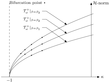
Figure 4: Schematic diagrams of local bifurcations on $\mathcal{T}_{\omega}^{+}|_{\beta_{j}}$ for $\beta_{1}>\beta_{2}>\beta_{3}>-1$.

Denote by $(\kappa_{j}(\beta),u_{\kappa_{j}(\beta)},v_{\kappa_{j}(\beta)})\in\mathcal{T}_{\omega}^{+}|_{\beta}$ the bifurcation point corresponding to

$$f(\beta)=\lambda_{j}(\kappa_{j}(\beta)).$$

By the monotonicity of $\lambda_{j}(\kappa)$, we have

$$-1<\kappa_{1}(\beta)<\kappa_{2}(\beta)<\cdots.$$

Based on these inequalities, (3.22) and the first part of proof of Lemma 3.9, one can easily get the following corollary.

Corollary 3.11.

Denote $(\kappa_{j}(\beta),u_{\kappa_{j}(\beta)},v_{\kappa_{j}(\beta)})\in\mathcal{T}_{\omega}^{+}|_{\beta}$ the bifurcation point corresponding to

$$f(\beta)=\lambda_{j}(\kappa_{j}(\beta)).$$

Then for each $j$, we have

$$\kappa_{j}(\beta)\rightarrow-1,\ \ \|u_{\kappa_{j}(\beta)}\|_{L^{2}}=\|v_{\kappa_{j}(\beta)}\|_{L^{2}}\rightarrow\infty,$$

as $\beta\rightarrow-1^{+}$.

4 Global bifurcations

Since each eigenvalue $\lambda_{j}(\kappa)$ of (3.19) has multiplicity one in $\mathcal{H}_{r}$. By Rabinowitz’s global bifurcation theorem [23], there is a global bifurcation branch emanates from $\mathcal{T}_{\omega}^{+}|_{\beta}$ at each bifurcation point. In this section, we shall discuss these global bifurcations.

In order to show the existence of positive bifurcation branches, we consider a modified system of (1.4),

$$\left\{\begin{array}[]{l}-\Delta u+u+\kappa v=(u^{+})^{3}+\beta uv^{2},\\ -\Delta v+v+\kappa u=(v^{+})^{3}+\beta u^{2}v,\\ u,v\in H_{r}^{1}(\mathbb{R}^{N}),\end{array}\right.$$ (4.1)

where $u^{+}=\max\{u,0\},u^{-}=\min\{u,0\}$. About the nontrivial solutions of (4.1), we have the following lemma.

Lemma 4.1.

For any $\beta\in(-1,0]$ and $\kappa\in(-1,0]$, the nontrivial solutions of (4.1) are positive, i.e., $u>0,v>0$ in $\mathbb{R}^{N}$.

Proof 4.2.

Multiply both sides of the first equation of (4.1) by $u^{-}$ and both sides of the second equation by $v^{-}$, then integrate on $\mathbb{R}^{N}$,

$$\|u^{-}\|^{2}+\int\kappa u^{-}v^{-}\leq\|u^{-}\|^{2}+\int\kappa u^{-}v =\beta\int(u^{-})^{2}v^{2}\leq 0,$$

$$\|v^{-}\|^{2}+\int\kappa u^{-}v^{-}\leq\|v^{-}\|^{2}+\int\kappa uv^{-} =\beta\int u^{2}(v^{-})^{2}\leq 0.$$

Adding the above two inequalities together, and note $-1<\kappa\leq 0$ we get

$$(1+\kappa)(\|u^{-}\|^{2}+\|v^{-}\|^{2})\leq 0.$$

Therefore, $u\geq 0,v\geq 0$ in $\mathbb{R}^{N}$.

From the first equation of (4.1) and the non-negativity of $v$, we get

$$\Delta u-(1-\beta v^{2})u=-(u^{+})^{3}+\kappa v\leq 0.$$

By the strong maximum principle, $u>0$ in $\mathbb{R}^{N}$. Similarly, $v>0$ in $\mathbb{R}^{N}$.

According to Lemma 4.1, it is easy to see that nontrivial solutions of (4.1) are positive solutions of (1.4). On the other hand, nonnegative solutions of (1.4) are also solutions of (4.1). In particular, the synchronized solution branch $\mathcal{T}_{\omega}^{+}|_{\beta}$ of (1.4) is a solution branch of system (4.1), and there exists a sequence of bifurcation solutions of (4.1) along $\mathcal{T}_{\omega}^{+}|_{\beta}$.

Remark 4.3.

Denote by $\mathcal{S}_{l}^{\beta}$ the global bifurcation branch of (4.1) emanating from $\mathcal{T}_{\omega}^{+}|_{\beta}$ at the $l$-th bifurcation point $(\kappa_{l},u_{\kappa_{l}},v_{\kappa_{l}})$. Lemma 4.1 implies that if $\beta\in(-1,0]$ fixed, then for any $(\kappa,u,v)\in\mathcal{S}_{l}^{\beta}$ with $-1<\kappa\leq 0$, there holds $u>0,v>0$. By the relation between (1.4) and (4.1), system (1.4) has a global bifurcation branch with positive components for fixed $\beta\in(-1,0]$ and parameter $\kappa\in(-1,0]$. Whereas, the bifurcation branches with respect to $\mathcal{T}_{\omega}^{+}|_{\beta}$ may continue beyond $\kappa=0$.

Proof of Theorem 1.4   It follows from Lemma 3.4, Lemma 3.9, Corollary 3.11, Lemma 4.1 and Remark 4.3. $\blacksquare$

Remark 4.4.

It is well known that a global bifurcation branch, in the sense of Rabinowitz, either is unbounded in the product space or contains multiple bifurcation points on $\mathcal{T}_{\omega}^{+}|_{\beta}$. In [5, 27, 28], there are some descriptions in this respect. So far, corresponding result for $\kappa$-bifurcation of system (1.4) or (4.1) is still unknown.

The first author is supported by the China Postdoctoral Science Foundation. The second author is supported in part by the National Natural Science Foundation of China 11325107, 11271353, 11331010.

References

- \bahao
- [1] Ambrosetti A, Cerami G, Ruiz D, Solitons of linearly coupled systems of semilinear non-autonomous equations on . J. Funct. Anal., 2008, 254: 2816–2845.
- [2] Ambrosetti A, Colorado E, Bound and ground states of coupled nonlinear Schrödinger equations. C. R. Math. Acad. Sci. Paris, 2006, 342: 453–458.
- [3] Ambrosetti A, Colorado E, Standing waves of some coupled nonlinear Schrödinger equations. J. Lond. Math. Soc., 2007, 75: 67–82.
- [4] Bartsch T, Bifurcation in a multicomponent system of nonlinear Schrödinger equations. J. Fixed Point Theory Appl., 2013, 13: 37–50.
- [5] Bartsch T, Dancer E N, Wang Z Q, A Liouville theorem, a-priori bounds, and bifurcating branches of positive solutions for a nonlinear elliptic system. Calc. Vari. Part. Diff. Equ., 2010, 37: 345–361.
- [6] Bartsch T, Wang Z Q, Note on ground states of nonlinear Schrödinger systems. J. Part. Diff. Equ., 2006, 19: 200–207.
- [7] Bartsch T, Wang Z Q, Wei J C, Bound states for a coupled Schrödinger system. J. Fixed Point Theory Appl., 2007, 2: 353–367.
- [8] Dancer E N, Wang K L, Zhang Z T, Uniform Hölder estimate for singularly perturbed parabolic systems of Bose-Einstein condensates and competing species. J. Differential Equations, 2011, 251: 2737–2769.
- [9] Dancer E N, Wang K L, Zhang Z T, The limit equation for the Gross-Pitaevskii equations and S. Terracini’s conjecture. J. Funct. Anal., 2012, 262: 1087–1131.
- [10] Dancer E N, Wang K L, Zhang Z T, Addendum to “The limit equation for the Gross-Pitaevskii equations and S. Terracini’s conjecture”[J. Funct. Anal. 262 (3) (2012) 1087-1131]. J. Funct. Anal., 2013, 264: 1125–1129.
- [11] Dancer E N, Wei J C, Weth T, A priori bounds versus multiple existence of positive solutions for a nonlinear Schrödinger system. Ann. Inst. H. Poincaré Anal. Non Linéaire, 2010, 27: 953–969.
- [12] Esry B D, Greene C H, Burke Jr J P, Bohn J L, Hartree-Fock theory for double condensates. Phys. Rev. Lett., 1997, 78: 3594–3597.
- [13] Gidas B, Spruck J, Gloal and local behavior of positive solutions of nonlinear elliptic equations. Commun. Pur. Appl. Math., 1997, 34: 525–598.
- [14] Lin T C, Wei J C, Ground state of Coupled Nonlinear Schrödinger equations in . Commun. Math. Phys., 2005, 255: 629–653.
- [15] Lin T C, Wei J C, Solitary and self-similar solutions of two-component system of nonlinear Schrödinger equations. Physics D: Nonlinear Phenomena, 2006, 220: 99–115.
- [16] Liu Z L, Wang Z Q, Multiple bound states of nonlinear Schrödinger systems. Comm. Math. Phy., 2008, 282: 721–731.
- [17] Liu Z L, Wang Z Q, Ground states and bound states of a nonlinear Schrödinger system. Advanced Nonlinear Studies, 2010, 10: 175–193.
- [18] Maia L A, Montefusco E, Pellacci B, Positive solutions for a weakly coupled nonlinear Schrödinger system. J. Diff. Equ., 2006, 299: 743–767.
- [19] Mawhin J, Willem M, Critical point theory and Hamiltonian system. Spinger-Verlag, New York, 1989.
- [20] Mitchell M, Chen Z, Shih M, Segev M, Self-trapping of partially spatially incoherent light. Phys. Rev. Lett., 1996, 77: 490–493.
- [21] Noris B, Tavares H, Terracini S, Verzini G, Uniform Hölder bounds for nonlinear Schrödinger systems with strong competition. Comm. Pure Appl. Math., 2010, 63: 267–302.
- [22] Noris B, Tavares H, Terracini S, Verzini G, Convergence of minimax and continuation of critical points for singularly perturbed systems. J. Eur. Math. Soc., 2012, 14: 1245–1273.
- [23] Rabinowitz P H, Some global results for nonlinear eigenvalue problems. J. Func. Anal., 1971, 7: 487–513.
- [24] Rüegg C, Cavadini N, Furrer A, Güdel H.-U., Krämer K, Mutka H, Wildes A, Habicht K, Vorderwischu P, Bose-Einstein condensation of the triplet states in the magnetic insulator TlCuCl3. Nature, 2003, 423: 62–65.
- [25] Sirakov B, Least energy solitary waves for a system of nonlinear Schrödinger equations in . Comm. Math. Phys., 2007, 271: 199–221.
- [26] Tian R S, Wang Z Q, Multiple solitary wave solutions of nonlinear Schrödinger systems. Topo. Mat. Non. Anal., 2011, 37: 203–223.
- [27] Tian R S, Wang Z Q, Bifurcation results on positive solutions of an indefinite nonlinear elliptic system. Disc. Cont. Dyna. Sys. - Series A, 2013, 33: 335–344.
- [28] Tian R S, Wang Z Q, Bifurcation results on positive solutions of an indefinite nonlinear elliptic system II. Adv. Non. Stud., 2013, 13: 245–262.
- [29] Wei J C, Weth T, Nonradial symmetric bound states for a system of two coupled Schrödinger equations. Rend. Lincei Mat. Appl., 2007, 18: 279–293.