Extreme Thouless effect in a minimal model of dynamic social networks

Abstract

In common descriptions of phase transitions, first order transitions are characterized by discontinuous jumps in the order parameter and normal fluctuations, while second order transitions are associated with no jumps and anomalous fluctuations. Outside this paradigm are systems exhibiting ‘mixed order transitions’ displaying a mixture of these characteristics. When the jump is maximal and the fluctuations range over the entire range of allowed values, the behavior has been coined an ‘extreme Thouless effect’. Here, we report findings of such a phenomenon, in the context of dynamic, social networks. Defined by minimal rules of evolution, it describes a population of extreme introverts and extroverts, who prefer to have contacts with, respectively, no one or everyone. From the dynamics, we derive an exact distribution of microstates in the stationary state. With only two control parameters, $N_{I,E}$ (the number of each subgroup), we study collective variables of interest, e.g., $X$, the total number of $I$-$E$ links and the degree distributions. Using simulations and mean-field theory, we provide evidence that this system displays an extreme Thouless effect. Specifically, the fraction $X/\left(N_{I}N_{E}\right)$ jumps from $0$ to $1$ (in the thermodynamic limit) when $N_{I}$ crosses $N_{E}$, while all values appear with equal probability at $N_{I}=N_{E}$.

I Introduction

In systems with many interacting degrees of freedom, interesting collective phenomena are associated with phase transitions, e.g., in ferromagnetism. Here, a suitable macroscopic variable characterizing the state of the system – the order parameter – typically changes its behavior in some rather dramatic fashion. In standard textbooks, phase transitions are classified by the Ehrenfest scheme: first order, second order, etc. We also learn to expect certain characteristics associated with each order. Thus, across the first order transition, the order parameter jumps, while its fluctuations are ‘normal’ (on either side). Metastability, hysteresis, and co-existence are other common features associated with this kind of transition. By contrast, opposite characteristics, e.g., no discontinuity and anomalously large fluctuations, are associated with second order transitions.

Though such properties are observed in most physical systems, there are exceptions. In the context of one-dimensional Ising models with long range interactions, Thouless Thouless (1969); Aizenman et al. (1988); Luijten and Meßingfeld (2001) found ‘mixed order’ transitions, at which the order parameter jumps discontinuously and exhibits large fluctuations. Since then, several systems with such properties have been discovered Blossey and Indekeu (1995); Poland and Scheraga (1966); Fisher (1966); Kafri et al. (2000); Gross et al. (1985); Schwarz et al. (2006); Toninelli et al. (2006). In particular, the term ‘extreme Thouless effect’ was coined recently Bar and Mukamel (2014a, b) to describe a case where, at the transition, both the jump and the fluctuations are maximal. In this paper, we report another system displaying such an effect, in the context of a minimal model of social interactions, involving dynamic networks with preferred degrees.

In our previous studies of such networks Liu et al. (2013, 2014), we introduced the notion that an individual (i.e., node) adds/cuts links to others according to its ‘preferred degree’: $\kappa$. The evolution of the simplest version of such networks is: In each time step, a random node is chosen and its degree, $k$, is noted. If $k>\kappa$, the node cuts one of its existing links at random. Otherwise, it adds a link to a randomly chosen node not connected to it. In the steady state of a homogeneous system (all nodes assigned the same $\kappa$), this ensemble of apparently random graphs displays quite different properties Zia et al. (2011) from the standard Erdős-Rényi case Erdős and Rényi (1959). Taking a small step towards describing an inhomogeneous society, we consider a heterogeneous system of two subgroups, with $N_{1,2}$ nodes assigned different $\kappa$’s. Letting $\kappa_{1}<\kappa_{2}$, we naturally refer to the first group as ‘introverts’ ($I$) and the latter one as ‘extroverts’ ($E$). Despite the simplicity of its rules, such a system exhibits a rich variety of properties, discovered mainly through simulations Liu et al. (2014). On the analytic front, progress has been modest, since the underlying dynamics violates detailed balance and the stationary state will have non-trivial persistent probability currents Zia and Schmittmann (2007). Under these circumstances, to gain some insight, we turn to limiting cases which embody the main features of the full system. In this spirit, we consider the ultimate limit: $\kappa_{1}=0,\kappa_{2}=\infty$. In other words, these are extreme introverts and extroverts (or $XIE$, for short). Specifically, we are able to find an exact expression for the stationary distribution, obtain analytic predictions for various quantities which are confirmed by simulations, and provide good evidence that the transition across $N_{1}=N_{2}$ displays an extreme Thouless effect. While preliminary results have been reported earlier Zia et al. (2012); Liu et al. (2012), we will present a more detailed study of this model here.

First, for the readers’ convenience, we provide a summary of the preliminary findings, by including a complete description of the model, the master equation associated with the stochastic process, the exact microscopic distribution in the steady state, and a mapping to an two-dimensional Ising model with peculiar interactions. In Section III, we study the statistical properties of $X$ (the total number of I-E links), an ‘order parameter’ which corresponds to the magnetisation of the Ising model. Using Monte Carlo techniques, we report findings much beyond those in ref. Zia et al. (2012); Liu et al. (2012): including a power spectrum study of the time traces of X, as well as some first steps towards a finite size analysis for X, as a function of $N_{I,E}$ (the number of I,E’s). These provide further evidence for the principal characteristics associated with an extreme Thouless effect. The following section is devoted to investigations of a standard characterization of networks: degree distributions. In the Ising language, these correspond to novel measures of the system, offering a more detailed picture than the magnetisation. For systems with $N_{I}\neq N_{E}$, predictions (i.e., no fitting parameters) of a self-consistent mean-field theory are largely confirmed by simulations. We end with a summary and outlook, while the Appendices contain many of the technical details.

II The $XIE$ model and the stationary distribution

With the motivations for this model presented in both the introduction and previous studies Zia et al. (2012); Liu et al. (2012), we provide the specifications of our model, using the language of a social network. Our population consists of $N$ individuals, divided into two groups: $N_{I}$ introverts and $N_{E}$ extroverts. Their behavior is ‘extreme,’ in the sense that the former/latter prefers contacts to none/everyone. The rules of evolution cannot be simpler:

• In each time step, a random individual is chosen.

• If an introvert is chosen, it cuts a random existing link.

• If an extrovert is picked, it adds a link to a random individual not already connected to it.

Note that one link changes at every step, except when the chosen individual is ‘content,’ i.e., a totally isolated $I$ or a fully connected $E$. Obviously, such a contented pair cannot be present simultaneously in our model. In this sense, our system may be termed ‘maximally frustrated,’ a measure Liu et al. (2014) we will not pursue here.

In simulation studies, it is customary to define one Monte Carlo Step (MCS) as $N$ such attempts, so that each node has an even chance of being chosen after $N$ attempts. Our main interest will be the statistical properties of this system at long times, once it settles into the stationary state. We emphasize again that, in this minimal model, there are just two control parameters: $N_{I,E}$. For large $N$, we may consider different ‘thermodynamic’ limits, e.g., fixed difference $N_{E}-N_{I}$ or ratio $N_{E}/N_{I}$. Note also that, though the total number of links can reach $N\left(N-1\right)/2$, the maximum number of cross-links between the two groups is

$$\mathcal{N}\equiv N_{I}N_{E}$$ (1)

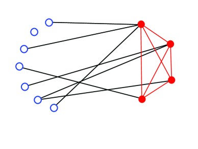
Figure 1: (Color online) The nodes of the two groups are denoted by circles: blue open ($I$) and red closed ($E$). The black lines represent the active cross-links and the red dashed lines, the frozen $E$-$E$ links. For this network, the sets of $k$’s are: $k_{I}=\left\{1,0,1,1,1,2,1\right\}$, and $k_{E}=\left\{6,5,4,4\right\}$. Thus, this configuration contributes $1,5,1$ to $\rho_{I}$ ($k=0,1,2$) and $2,1,1$ to $\rho_{E}$ ($k=4,5,6$), respectively.

Clearly, regardless of how the system is initialized, all the intra-communities links ($I$-$I$ or $E$-$E$) will quickly become static (all absent or present). Only the $I$-$E$ cross-links are dynamic, depending on which node happens to be chosen (illustrated in Fig. 1). In other words, we may limit our attention to the set of bipartite graphs. Of course, the total number of cross-links, $X$ ($\in\left[0,\mathcal{N}\right]$), fluctuates and should display interesting statistical properties. The first impression of such a minimal model is that it must be trivial. In particular, it may be argued that, since the probability for a link to be cut or added is proportional to $N_{I}/N$ or $N_{E}/N$, the fraction

$$x\equiv X/\mathcal{N}$$ (2)

should be simply $N_{E}/N$. In the rest of this article, we will show the behavior of $x$ to be dramatically different.

The configuration space here consists of the $N_{I}\times N_{E}$ incidence matrices, $\mathbb{N}$. We denote its elements by $n_{ij}$ ($i\in\left[1,N_{I}\right],j\in\left[1,N_{E}\right]$) which is $1\,$or $0$ when the link between an introvert node $i$ and an extrovert $j$ is present or absent, respectively. Clearly, this configuration space is identical to that of a $N_{I}\times N_{E}$ Ising model on a square lattice. Following the lattice gas language Yang and Lee (1952), we will refer to $n=1,0$ as a ‘particle’ or a ‘hole.’ Meanwhile, the dynamics of cutting/adding corresponds to a kinetic Ising model with spin flip dynamics Glauber (1963) (i.e., without particle conservation). Since $X=\Sigma_{ij}n_{ij}$ and $\mathcal{N}$ is the total number of sites in the Ising system, we have the mapping

$$x=\left(1+m\right)/2$$ (3)

where $m\in\left[-1,1\right]$ is the magnetisation. To further this correspondence, let us define

$$h\equiv\Delta/N;~{}~{}\Delta\equiv N_{E}-N_{I}$$ (4)

with $h$ playing the role of the magnetic field. Thus, our interest in how $x$ responds to $N_{I,E}$ translates into finding a ‘equation of state’ $m\left(h\right)$. In this language, the naive expectation is trivial (and false): $m\left(h\right)=h$.

Of course, unlike in the Ising case, the statistical mechanics of the $XIE$ model is defined by dynamical rules rather than a Hamiltonian. Therefore, to study quantities of interest, we must first find the distribution of the stationary state, $\mathcal{P}^{ss}\left(\mathbb{N}\right)$, as opposed to just writing a Boltzmann factor.

With the dynamics specified, we can write the master equation for $\mathcal{P}(\mathbb{N},t)$, the probability of finding the system in configuration $\mathbb{N}$ at time $t$:

$$\mathcal{P}(\mathbb{N},t+1)-\mathcal{P}(\mathbb{N},t)=$$

$$\qquad\sum_{\{\mathbb{N}^{\prime}\}}[W(\mathbb{N},\mathbb{N}^{\prime})\mathcal{P}(\mathbb{N}^{\prime},t)-W(\mathbb{N}^{\prime},\mathbb{N})\mathcal{P}(\mathbb{N},t)]$$ (5)

where $W(\mathbb{N}^{\prime},\mathbb{N})$ is the probability for configuration $\mathbb{N}$ to become $\mathbb{N}^{\prime}$ in a step (an attempt). For $W$, we note that the dynamics for an $I$ node $i$ involves cutting a random existing link, so that $k_{i}$, the number of links it has (i.e., particles in row $i$ in $\mathbb{N}$) will be needed. Similarly, for a $E$ node $j$, we will need $p_{j}$, the number of holes in column $j$ in $\mathbb{N}$. Letting $\bar{n}_{ij}\equiv 1-n_{ij}$, we define

$$k_{i}\equiv\Sigma_{j}n_{ij};~{}~{}p_{j}\equiv\Sigma_{i}\bar{n}_{ij}$$ (6)

Clearly, these variables reveal a not-so-explicit symmetry in the dynamics of $XIE$. Similar to the Ising spin flip symmetry ($n\Leftrightarrow\bar{n}$), there is an additional, transpose operation:

$$n_{ij}\Leftrightarrow\bar{n}_{ji}\oplus N_{I}\Leftrightarrow N_{E}$$ (7)

We will refer to this, à la Ising, as ‘particle-hole symmetry,’ which will play an important role in discussions below. A layman’s way to phrase this symmetry is: The presence of a link is as intolerable to an introvert as the presence of a ‘hole’ is to an extrovert.

With these preliminaries, the $W(\mathbb{N}^{\prime},\mathbb{N})$ in Eqn. (5) reads

$$\sum\limits_{i,j}\left[\frac{\Theta\left(k_{i}\right)}{k_{i}}\bar{n}_{ij}^{\prime}n_{ij}+\frac{\Theta\left(p_{j}\right)}{p_{j}}n_{ij}^{\prime}\bar{n}_{ij}\right]\frac{\Pi_{k\ell\neq ij}\delta\left(n_{k\ell}^{\prime},n_{k\ell}\right)}{N}$$ (8)

where $\Theta\left(x\right)$ is the Heavyside function (i.e., $1$ if $x>0$ and $0$ if $x\leq 0$) and the product of $\delta$’s ensures that only one $n_{ij}$ may change in a step. It is straightforward to verify that Eqn. (5) respects particle-hole symmetry.

The dynamics defined by Eqn. (5) is clearly ergodic. More remarkably, unlike those in less extreme models of introverts and extroverts Liu et al. (2013, 2014), it obeys detailed balance (shown in Appendix A). Consequently, in the $t\rightarrow\infty$ limit, $\mathcal{P}$ approaches a unique stationary distribution, which can be found by applying $\mathcal{P}^{ss}\left(\mathbb{N}\right)=\mathcal{P}^{ss}\left(\mathbb{N}^{\prime}\right)W\left(\mathbb{N},\mathbb{N}^{\prime}\right)/W\left(\mathbb{N}^{\prime},\mathbb{N}\right)$ repeatedly. Imposing normalization, we arrive at an explicit, closed form:

$$\mathcal{P}^{ss}\left(\mathbb{N}\right)=\frac{1}{\Omega}\prod\limits_{i=1}^{N_{I}}\left(k_{i}!\right)\prod\limits_{j=1}^{N_{E}}\left(p_{j}!\right)$$ (9)

where $\Omega=\Sigma_{\left\{\mathbb{N}\right\}}\Pi\left(k_{i}!\right)\Pi\left(p_{j}!\right)$ is a ‘partition function.’ Note that the particle-hole symmetry (Eq. 7) is manifest here.

Interpreting $\mathcal{P}^{ss}$ as a Boltzmann factor and trivially assuming $\beta=1$, we can write a ‘Hamiltonian’

$$\mathcal{H}\left(\mathbb{N}\right)=-\left\{\sum\limits_{i=1}^{N_{I}}\ln\left(\sum\limits_{j=1}^{N_{E}}n_{ij}\right)!+\sum\limits_{j=1}^{N_{E}}\ln\left(\sum\limits_{i=1}^{N_{I}}\bar{n}_{ij}\right)!\right\}$$ (10)

Now, this expression immediately alerts us to the level of complexity of this system of ‘Ising spins,’ as $\mathcal{H}$ contains a peculiar form of long range interactions. Each ‘spin’ is coupled to all other ‘spins’ in its row and column, via all possible types of ‘multi-spin’ interactions! We are not aware of any system in solid state physics with this kind of interactions. It is remarkable that such a complex $\mathcal{H}$ emerges from an extremely simple model of social interactions. Meanwhile, it is understandable that computing $\Omega$, let alone statistical properties of macroscopic quantities, will be quite challenging (Appendix B). Nevertheless, as the next two sections show, we are able to exploit mean-field approaches to gain some insight, and to predict some macroscopic observables. For generic $\left(N_{I},N_{E}\right)$, we find excellent agreement with simulation data. As in standard equilibrium statistical systems, these theories fail in the neighborhood of critical points, which turn out to be the $N_{I}=N_{E}$ line here.

III Statistics of $X$, the total number of cross-links

In the $XIE$ model, the most natural macroscopic quantity to study is $X$, the total number of $I$-$E$ links. In addition, its average $\left\langle X\right\rangle$ can serve as an ‘order parameter,’ since it plays the role of the total magnetisation in the Ising model. Though there is no natural temperature-like variable in our model of social networks, there is a natural external-field-like control parameter: $h$ (or $\Delta$). Our main interest in this section is how $\left\langle X\right\rangle$ varies with $N_{I,E}$. In other words, what is the ‘equation of state’ $m\left(h;\mathcal{N}\right)$ for the $XIE$ model? If it were like the Ising model below criticality, $m\left(h=0_{\pm};\mathcal{N}\rightarrow\infty\right)=\pm m_{s}$, where $0<m_{s}<1$ is the spontaneous magnetisation, accompanied by ordinary $O\left(1/\sqrt{\mathcal{N}}\right)$ fluctuations. In the Thouless effect, a discontinuity would be accompanied by anomalously large fluctuations. Here, we will find that our $m$ displays an extreme Thouless effect in the thermodynamic limit, i.e., $m\left(h=0_{\pm};\mathcal{N}\rightarrow\infty\right)=\pm 1$, together with extraordinary, $O\left(1\right)$, fluctuations around $m\left(h=0\right)=0$.

The preliminary results for $N=200$, displayed in Figs. 1-3 in Liu et al. (2012) gave a hint of these remarkable properties. To confirm and to improve on those results, we carry out much longer runs: discarding the first $5\times 10^{7}$ MCS, taking measurements every $50$ MCS, for up to $10^{11}$ MCS (for the $N_{I,E}=100$ case). Using these long traces, $X\left(t\right)$, we find much more information than just the average $\left\langle X\right\rangle$; we obtain a much more accurate picture for the whole steady state distribution $P\left(X\right)$: Fig. 2. Not surprisingly, they are sharply peaked and Gaussian-like for the off-critical cases (green and blue on line), while the distribution in the $N_{I}=N_{E}$ case (red on line) is essentially flat over most of the full range, $\left[0,\mathcal{N}\right]$. The flat plateau in $P\left(X\right)$ gives the impression of an unbiased random walk (bounded by ‘soft’ walls near the extremes of the allowed region). In stark contrast, characteristic of co-existence in an ordinary first order transition, $M\left(t\right)$ for an Ising system below criticality spends much of its time hovering around the spontaneous magnetizations, $\pm M_{sp}$, and makes rare and short excursions from one to the other.

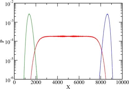
Figure 2: (Color online) The distributions, $P\left(X\right)$, compiled with the time traces of $X$ for three cases with $\left(N_{I},N_{E}\right)$ near and at criticality: $\left(101,99\right)$ (green dashed line), $\left(99,101\right)$ (blue dot-dashed line), and $\left(100,100\right)$ (red solid line).

Another principal characteristic is metastability or hysteresis. Though not shown explicitly here, we observe neither. When the two nodes ‘change sides,’ i.e., $\left(101,99\right)\rightarrow\left(99,101\right)$, $X/\mathcal{N}$ simply marches from $\thicksim 15\%$ to $\thicksim 85\%$ in $\thicksim 3500$ MCS. In other words, on the average, $X$ changes by about two links per MCS. We also considered having $\delta=4$ or $6$ ‘defectors’ instead of just two, in systems with $N=400$ and $800$. In all cases, the average ‘velocity’ is approximately $\delta$ per MCS. Intuitively, we may attribute this to the action of the $\delta$ extra $E$ nodes, but it remains to be shown analytically. In all respects, there is absolutely no barrier between the two extremes of $X$ ! As for criticality itself $\left(100,100\right)$, the notion of $X$ executing a pure random walk (RW) can be further confirmed by studying its power spectrum. With $\mathcal{T}=2\times 10^{4}$ measurements (of runs of $2\times 10^{6}$ MCS), we compute the Fourier transform $X\left(\omega\right)$ and then average over 100 runs to obtain $I\left(\omega\right)\equiv\left\langle\left|X\left(\omega\right)\right|^{2}\right\rangle$. In Fig. 3, we show plots of $\log I$ vs. $\log\omega$, as well a straight line (black dashed) representing $\omega^{-2}$. The upper set of data points (red on line), associated with $N_{I}=N_{E}=100$, are statistically consistent with the RW characteristic of $\omega^{-2}$. The cutoff at small $\omega$ can be estimated from the finite range available to the RW ($\thicksim 7000$ here). Since $\Delta X=\pm 1$ in each attempt, we can assume the traverse time to be about $7000^{2}\cong 5\times 10^{7}$ attempts, or $\thicksim 2.5\times 10^{5}$ MCS. Given that this value is comparable to $1/10$ of our run time, it is reasonable to expect deviations from the pure $\omega^{-2}$ as we approach $\omega\thicksim 10$. By contrast, the power spectra of the two off-critical cases (lower set of data, green and blue on line) are controlled by some intrinsic time scale associated with both the restoration to $\left\langle X\right\rangle$ and the fluctuations thereabout. Indeed, this $I\left(\omega\right)$ is entirely consistent with a Lorentzian, i.e., $\propto 1/\left(\omega^{2}+\omega_{0}^{2}\right)$. Given our limited understanding of the dynamics of this model, estimating $\omega_{0}$ is beyond the scope of this work.

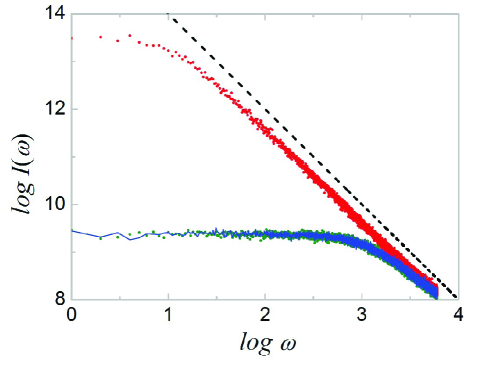
Figure 3: (Color online) Power spectra, $I\left(\omega\right)$, associated with the time traces of $X(t)$. The dashed black line is proportional to $1/\omega^{2}$. Note that the spectra associated with the two off-critical cases (farthest from the dashed line, shown as green dots and a blue line) are statistically identical, as expected from particle-hole symmetry. Both scales are $log_{10}$.

As shown in ref. Liu et al. (2012), some characteristics of an extreme Thouless effect (presence of a jump, absence of metastability and hysteresis, existence of a flat plateau in $P\left(X\right)$, etc.) can be qualitatively understood in terms of a crude mean field approximation. That approach starts with the exact

$$P\left(X\right)\equiv\sum_{\left\{\mathbb{N}\right\}}\delta\left(X,\Sigma_{ij}n_{ij}\right)\mathcal{P}^{ss}\left(\mathbb{N}\right).$$ (11)

and replaces every $n_{ij}$ by its average $X/\mathcal{N}$ in the sum, resulting in an approximate $\tilde{P}\left(X\right)$. Its maximum can be used to predict $\left\langle X\right\rangle$ and so, an approximate equation of state $\tilde{m}\left(h;\mathcal{N}\right)$. Remarkably, at the lowest order in $1/\mathcal{N}$, this approach leads to an extreme Thouless effect Bar and Mukamel (2014a, b), i.e.,

$$\tilde{m}=sign\left(h\right),$$ (12)

the absence of metastability and hysteresis when $h$ changes sign, as well as a flat plateau in $\tilde{P}\left(X\right)$ for $h=0$! Keeping the next order in $\tilde{F}$, we find

$$\tilde{m}\left(h;N\right)=sign\left(h\right)-\frac{1}{hN}+...$$ (13)

which provides qualitatively good agreement with most of the $N=200$ data set. Clearly, this mean-field approach captures some key features of the $XIE$ model, even though it is not quantitatively reliable.

Before we turn to a much better mean field theory, let us present the rudiments of a more complete portrait, towards a systematic scaling study. Specifically, we study $m\left(h;N\right)$ in the transition region, using simulations with $N$ up to $3200$. Of course, unlike the Ising model, there is no natural variable in the social network corresponding to temperature. Nevertheless, the results suggest the presence of anomalous power laws and possible data collapse.

To study the behavior near criticality, we measure the average $\left\langle X\right\rangle$ for all possible values of $N_{I,E}$ which correspond to $h\leq 0.01$, with $N=200,400,...,3200$. In other words, we use the appropriate values of $\Delta=2,4,...32$. Starting with a half filled set of $I$-$E$ links, each point was calculated with a run of up to $5\times 10^{9}$ MCS with measurements made about every $N/4$ MCS. Verifying that our data is consistent with particle-hole symmetry, we present results only for $h>0$ and $m\cong 1$. Fig. 4a shows results within the small regime $h\in\left[0,0.01\right]$ and $m\in\left[0.7,1.0\right]$. We see that, indeed, $m\left(h;\mathcal{N}\right)$ approaches $+1$ as $N\rightarrow\infty$. Note that, we can access smaller $h$ in systems with larger $N$, as its minimum is $2/N$ . With this set of data, we make two log-log plots (Fig. 4b) showing that (i) for fixed $h=0.01$, $m\rightarrow 1$ with $N^{-0.71}$ and (ii) for fixed $\Delta=2$, $m\rightarrow 1$ with $N^{-0.36}$. The solid lines represent linear fits with correlation coefficient (R²) greater than 0.999. Using this information, we plot $N^{0.71}m$ against $h^{-0.34}$ in Fig. 4c. Though somewhat rough, this plot does qualitatively indicate data collapse and provides the first steps towards an in-depth finite size scaling analysis. Such a study is beyond the scope of this paper and will be reported elsewhere Bassler et al. (2014). If the exponents found here are confirmed, they signal a significant deviation from the mean-field values (e.g., Eq.13): $\left(0.70,0.36\right)$ as opposed to $\left(1,0\right)$. Of course, they also provide fertile ground for renormalization group analysis, along the lines of ref. Bar and Mukamel (2014a, b).

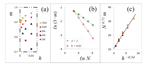
Figure 4: (Color online) (a) $m(h)$ for various $N$’s and allowed $\Delta$’s with $h\leq 0.01$. (b) Log-log plots of indicated subset of points in (a). Solid and dashed lines are linear fits with slope $-0.363$ and $-0.707$, respectively. Both correlation coefficients are greater than $0.999$. (c) Scaled plots of the points in (a), showing tolerable data collapse. Dashed line is linear, as guide to the eye.

IV Degree distributions: simulation results and a dynamic mean-field theory

In this section, we turn to a ‘mesoscopic’ quantity which offers a more detailed perspective than the macroscopic $X$, as well as major contrasts between Ising-like statistical systems and those associated with networks. For the Ising model, a natural quantity to study is the total magnetisation, which corresponds to $X$. But, it is not usual to study the statistics of the magnetisation in a row or a column. Yet, for the $XIE$ model, the corresponding quantity is the degree distribution, $\rho(k)$, which is one of the most common ways to characterise a network. Thus, we devote the rest of this paper to these distributions, illustrating with simulation data (for $N=200$), as well as offering a more effective mean-field theory. Specifically, unlike the mean-field approach for $\tilde{P}\left(X\right)$, we will formulate an approximate dynamics for $\rho$ and arrive at much better agreement with data, for all $N_{I}\neq N_{E}$. In particular, $\tilde{m}\left(0.01;200\right)$ above differs from data by $\thicksim 15\%$, while the theory below produces a value within 0.02%.

Before presenting the data, let us set the stage for discussing two degree distributions. In general, associated with a network with several subgroups or communities, we can study many such distributions, to describe the various intra- and inter-community links. For $XIE$, the intra-community links are static and so, we need to study only two: $\rho_{I}(k_{I})$ and $\rho_{E}(k_{E})$, related to the degrees of the $I$’s and $E$’s, respectively. To illustrate, a network with $\rho_{I}(1)=5$ and $\rho_{E}(6)=1$ is shown in Fig. 1. From the $\rho$’s, average degrees $\left\langle k_{I}\right\rangle$ and $\left\langle k_{E}\right\rangle$ can be found. Note that $\left\langle k_{I}\right\rangle\neq\left\langle k_{E}\right\rangle$ typically, but they are related, in the steady state, by the following. Since $N_{I}\left\langle k_{I}\right\rangle$ is just the average number of cross-links, while an extrovert has $k_{E}-N_{E}+1$ links to the $I$’s, we have

$$N_{I}\left\langle k_{I}\right\rangle=\left\langle X\right\rangle=N_{E}\left\langle k_{E}\right\rangle-N_{E}\left(N_{E}-1\right)$$ (14)

This complication can be bypassed, especially in view of the particle-hole symmetry discussed above, by introducing a ‘hole’ distribution for the $E$’s: $\zeta_{E}\left(p_{E}\right)$. Clearly, $\zeta$ is intimately related to $\rho$, namely, $\zeta\left(p\right)=\rho\left(N-1-p\right)$. Meanwhile, $N_{E}\left\langle p_{E}\right\rangle=\mathcal{N}-\left\langle X\right\rangle$, so that a manifestly symmetric constraint on $\rho,\zeta$ is $N_{I}\left\langle k_{I}\right\rangle+N_{E}\left\langle p_{E}\right\rangle=\mathcal{N}$.

Next, let us present the simulation results. Starting with a network with various initial conditions (null graph, complete graph, random half-filled), we evolve the system according to the simple rules given above. Not surprisingly, after $O\left(N\right)$ MCS, all the $I$-$I$ links are absent while all the $E$-$E$ links are present. To be quite certain that the system has equilibrated, we discard the first $5\times 10^{7}$ MCS. Thereafter, we measure the degrees of each node every $50$ MCS. The distributions are then obtained as the average over $10^{8}$ measurements. Shown in Fig. 5(a) are $\rho\left(k\right)$ for three cases: $\left(N_{I},N_{E}\right)=\left(150,50\right)$, $\left(125,75\right)$, $\left(101,99\right)$. Evidently, each $\rho$ consists of two components, associated with $k\leq N_{E}$ and $k\geq N_{E}-1$. Generally, these component are disjoint and so, they can be identified unambiguously with respectively, $\rho_{I}$ and $\rho_{E}$ (shown with open and solid symbols). Note that, in the $\left(101,99\right)$ case, despite having just two members less, the $\thicksim 100$ extroverts are unable to create enough cross-links, so that there are essentially no $I$’s with say, $50$ links! Of course, this result is entirely consistent with our observations above, showing that a typical $I$ has only about $15$ links. Apart from having these two components, the most prominent feature is that neither component resembles $3^{-\left|k-\kappa\right|}$, the degree distribution of a homogeneous population with preferred degree $\kappa$ Zia et al. (2011); Liu et al. (2013). As will be shown, they are well approximated by Poisson distributions, an analytic result of our mean-field theory.

 

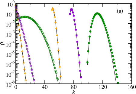
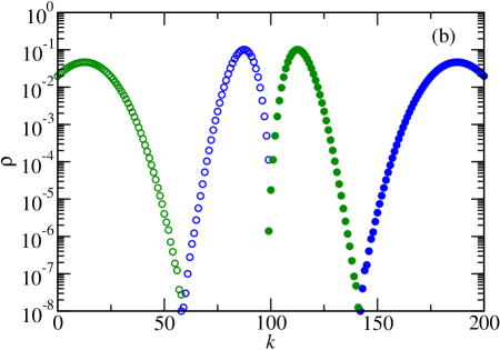
Figure 5: (Color online) Degree distributions, $\rho$, for several cases with $N_{I}+N_{E}=200$. Simulation results for the low/high $k$ components, associated with introverts/extroverts, are denoted by open/solid symbols. (a) The symbols for $(N_{I},N_{E})$ are orange triangles $(150,50)$, purple squares $(125,75)$, and green circles $(101,99)$. The solid black lines are predictions from a self-consistent mean-field theory. (b) When two introverts ‘change sides,’ a dramatic jump in $\rho\left(k\right)$ results, with the case of $(99,101)$ shown as blue diamonds.

What happens when the introverts ‘defect’? Though the changes appear dramatic, they should not be a surprise, given the underlying particle-hole symmetry in $XIE$. Thus, we illustrate in Fig. 5(b) the degree distribution for $(N_{I},N_{E})=(99,101)$ (blue circles), as well as the previous case of $(101,99)$ (green circles). By exchanging $N_{I}\Leftrightarrow N_{E}$ and plotting the degree distribution vs. $p\equiv N-1-k$, we find perfect (within statistical errors) overlap between the blue and green data points.

IV.1 Self-consistent mean-field approximation (SCMF)

Given the exact steady state distribution (Eq. 9), the $\rho$’s can be computed, in principle, from e.g., $\rho_{I}\left(k_{I}\right)=\sum_{\left\{\mathbb{N}\right\}}\delta\left(k_{I}-\Sigma_{j}n_{ij}\right)\mathcal{P}^{ss}\left(\mathbb{N}\right)$ (for any $i$). In practice, this task is as difficult as computing $P\left(X\right)$, so that we again resort to a mean-field approach. The main difference between the earlier scheme and this one is that the approximation will be applied to the underlying dynamics of the model Liu et al. (2013, 2014) (as opposed to evaluating the sum $\Sigma_{\left\{\mathbb{N}\right\}}$ above). In other words, we formulate an approximation on the transition probabilities – for the degree of a particular node to increase/decrease by unity: $R\left(k\rightarrow k\pm 1\right)$. Once these are determined, we impose the steady state condition

$$\tilde{\rho}\left(k\right)R\left(k\rightarrow k-1\right)=\tilde{\rho}\left(k-1\right)R\left(k-1\rightarrow k\right)$$ (15)

to find $\tilde{\rho}\left(k\right)$ (being an approximate $\rho$, again denoted by a tilde) in closed form. The strategy is as follows. Exploiting particle-hole symmetry, we will consider the two distributions, $\rho_{I}$ and $\zeta_{E}$, as well as two sets of rates, $R_{I,E}$. Each $R$ will depend on an unknown parameter, representing the average degree of the opposite community. From these, explicit expressions for $\tilde{\rho}_{I}$ and $\tilde{\zeta}_{E}$ can be obtained. In turn, the average degrees can be computed and the unknown parameters can now be fixed through self-consistency. In this spirit, we refer to this scheme as a SCMF approximation, details of which can be found in Appendix C. Here, we simply quote the results:

$$\tilde{\rho}_{I}\left(k_{I}\right)=\frac{\lambda^{N_{E}-k_{I}}}{Z_{I}\left(N_{E}-k_{I}\right)!};~{}~{}\tilde{\zeta}_{E}\left(p_{E}\right)=\frac{\mu^{N_{I}-p_{E}}}{Z_{E}\left(N_{I}-p_{E}\right)!}$$ (16)

where $\lambda,\mu$ are constants which can be obtained from $N_{I,E}$ alone and $Z$’s are normalization factors (Eqs. 30,36). Both are truncated Poisson distributions, since $k_{I}\in\left[0,N_{E}\right]$ and $p_{E}\in\left[0,N_{I}\right]$. Instead of quoting $\lambda$ and $\mu$ from the SCMF calculation, we plot the full distributions predicted by Eqs. (31,35), shown as solid black lines in Fig. 5(a). We should emphasize that no fit parameters have been introduced in this approach; the lines depend only on the control parameters, $N_{I,E}$. It is clear that the agreement between theory and simulation data is excellent for $N_{I}>N_{E}$. By symmetry, it will also be quite good for cases with $N_{I}<N_{E}$. Indeed, disagreement between theory and data is visibly detectable only in the tails of the next-to-critical case, $\left(101,99\right)$, a sign that correlations can no longer be entirely neglected here. From these distributions, we easily obtain $\left\langle X\right\rangle$ using Eq. (14). Unlike the results from the previous Section, all of these predictions fall within statistical errors of the data. Since mean field schemes are not the start of a systematic set of approximations, it is unclear why the approach here is so much more successful at capturing the essentials of the model.

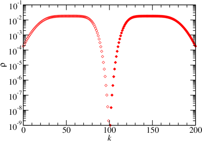
Figure 6: (Color online) Simulation results of the degree distribution for the symmetric $\left(100,100\right)$ case. The two components, denoted by open and solid diamonds, can be associated with the separate distributions $\rho_{I}$ and $\rho_{E}$, respectively.

To end this section, let us illustrate, with the symmetric case $(100,100)$, the challenges of ‘criticality.’ As expected, there are non-trivial obstacles for both Monte Carlo simulations and theoretical understanding. First of all, it takes much longer for the system to settle, typically a hundred-fold longer than the $N_{I}\neq N_{E}$ cases. To compile a reliable histogram for the $\rho\left(k\right)$, shown in Fig. 6, we take $10^{10}$ measurements in a combination of $5$ runs, each of which lasts for $10^{11}$ MCS (after discarding the first $10^{7}$ MCS for the system to settle into steady states). Note that, to untangle $\rho_{I,E}$ in the central pair of points, we recorded separately whether an $I$ or a $E$ node has $99$ or $100$ links. Of course, the distribution is symmetric, i.e., $\rho_{I}=\zeta_{E}$. Unlike the off-critical cases, these distributions display broad and flat plateaux. Undoubtedly, the physics underlying these also gives rise to the plateau in $P\left(X\right)$. Quantitative understanding of these large fluctuations remains elusive, while the SCMF prediction for this case is, not surprisingly, far from ideal.

V Summary and outlook

In this article, we report findings concerning an extraordinary phase transition in a minimal model of dynamic social networks with preferred degree. Consisting of extreme introverts/extroverts, who only cut/add connections, these dynamic networks have only the $I$-$E$ links and reduce to bipartite graphs. With only two control parameters, $N_{I,E}$, this seemingly trivial model displays surprising behavior. In particular, we find compelling evidence that, in the limit of large populations, (i) the likelihood of a link being present, $\left\langle x\right\rangle$, jumps discontinuously, from $0$ to $1$, when $N_{I}$ drops below $N_{E}$ and (ii) in the $N_{I}=N_{E}$ case, $x$ assumes all values in $\left[0,1\right]$ with equal probability. Such remarkable properties have been observed in other statistical systems, e.g., 1D Ising models with certain long range interactions Bar and Mukamel (2014a, b). We can place the similarity between our dynamic $XIE$ model and equilibrium Ising systems on firmer grounds, by mapping their microscopic configurations one-to-one and regarding the evolution of the former as Glauber spin-flip dynamics on the latter. Thanks to restoration of detailed balance, we are able to find an exact expression for the $XIE$ stationary distribution, $\mathcal{P}^{ss}$. Interpreting it as a Boltzmann factor, $-\ln\mathcal{P}^{ss}$ can be regarded as a ‘Hamiltonian’ for the spins, though much more complex than typical Ising models. Statistical properties of our system can now be explored along standard routes.

To study of the collective behavior arising from such microscopics, we focus on the degree distributions and $x$, the fraction of cross-connections. Since $x$ corresponds to $m$ (the magnetisation in the Ising model), while $h\,$or $\Delta$ (Eq. 4) can serve as an external magnetic field, a natural question for us is: What is the ‘equation of state,’ $m\left(h\right)$? Though naive expectations lead to the trivial $m=h$, both simulations and mean field theories point towards the contrary: $m=sign\left(h\right)$, which is a hallmark of an extreme Thouless effect Bar and Mukamel (2014a, b). Apart from the macroscopic $X$, we also study degree distributions $\rho\left(k\right)$, ‘mesoscopic’ quantities which are commonly used in characterizing networks. Remarkably, the predictions from a mean field approximation, formulated at the level of the underlying dynamics for $\rho\left(k,t\right)$, are in excellent agreement with data (for all $N_{I}\neq N_{E}$).

The results of this first study are encouraging and provide us with good stepping stones towards more systematic investigations. The most obvious question may be what forms do thermodynamic limits take, assuming they exist. Preliminary studies Dhar and Zia (2014) suggest that, for fixed $h$, the degree distributions (16) approach non-trivial limits. On the other hand, if $\Delta$ were held fixed instead, it is unclear what the limiting behavior is. How the system approach such limits is the next issue. A detailed study of finite size scaling should be undertaken Bassler et al. (2014), using both simulations and theoretical techniques. Pursuing an exact computation of the partition function, and perhaps $P\left(X\right)$, poses a worthy challenge. The failure of mean-field theory, especially near ‘criticality’ hints at the importance of correlations. However, there is no spatial structure in our model and so, the usual notion of correlation length is ill defined. Nevertheless, we have some evidence of strong correlations, in the sense that the joint distribution, $\rho\left(k_{I},k_{E}\right)$, can be quite different from the product $\rho_{I}\left(k_{I}\right)\rho_{E}\left(k_{E}\right)$. Systematic investigations of them are straightforward and worthwhile. From a theoretical point of view, it would be desirable to develop an understanding for why the SCMF is so much more successful than the standard mean-field approach (Section III). Such insights may have impact beyond this study, as they may reveal how best to formulate mean-field approximations.

Beyond exploring these questions, we can extend the $XIE$ model in an orthogonal direction, arguably of purely theoretical interest (at present). We may treat $\mathcal{H}$ as a genuine Hamiltonian in a standard study of critical phenomena in thermal equilibrium. In other words, we propose to study the statistical mechanics of a $L\times L$ system associated with the Boltzmann factor

$$\mathcal{P}\propto\exp\left\{-\beta\left[\mathcal{H}-BX\right]\right\}$$ (17)

Here, $\beta$ is the usual inverse temperature variable, while the bias $B$ plays the role of a symmetry breaking, ‘magnetic field’ (similar, but not identical to $h$ in the $XIE$). It is interesting to note that, while the critical control parameters of a typical system (e.g., $T_{c}$ in Ising, $T_{c}$ and $p_{c}$ for liquid gas) are not known, they are given precisely by $\beta_{c}=1$ and $B_{c}=0$ here. For this ‘purely theoretical’ system, work is in progress Bassler et al. (2014), to explore the usual avenues of interest: static and dynamic critical exponents, scaling functions, universality and the classes, etc. In the language of renormalization group analyses (which proved to be highly effective in dealing with other mixed-order transitions Cardy (1981); Bar and Mukamel (2014a)), we already know that $\mathcal{H}$ lies on the critical sheet and can inquire about fixed points and their neighborhoods, irrelevant and relevant variables (e.g., if there are others besides $\beta-1$ and $B$), etc. In addition, there are unusual challenges, such as the lack of a natural correlation length in such a system.

Beyond the $XIE$ model and its purely theoretical companion, there is a wide vista involving dynamic networks with preferred degrees. For instance, instead of assigning one or two $\kappa$’s to a population Liu et al. (2013, 2014), it is more natural to assign a distribution of $\kappa$’s. There are also multiple ways to model interactions between the various groups. For example, even with just two groups, it is realistic to believe that an individual may have two preferred degrees, one for contacts within the group and another for those outside. Surely, this kind of differential preference underlies the formation of social cliques. Beyond understanding the topology and dynamics of interacting networks of the types described here, the next natural step is to take into account the freedom associated with the nodes, e.g., opinion, wealth, health, etc., on the way to the ambitious goal of understanding adaptive, co-evolving, interdependent networks in general. Along the way, we can expect the unexpected, such as the emergence of the extreme Thouless effect in this $XIE$ model, arguably the simplest of all interacting social networks.

Appendix A Restoration of detailed balance

In this appendix, we show that all Kolmogorov loops are reversible in the XIE model and so, detailed balance is restored Kolmogorov (1936). Since the full dynamics occurs on the $\mathcal{N}$ cross-links, the configuration space consists of the corners of an $\mathcal{N}$-dimensional unit cube, while adding/cutting a link is associated with traversing an edge therein. Clearly, products of the ratios of forward and reversed transition rates around any closed loop can be expressed in terms of those around ‘elementary loops’ – i.e., loops around a plaquette on the $\mathcal{N}$-cube. We will show that the ratio associated with every plaquette is unity and so, all Kolmogorov loops are reversible.

First, it is easy to see that if an elementary loop consists of modifying two links connected to four different nodes, then the actions on each link are unaffected by the other. In other words, rates associated with opposite sides of the square (loop) are the same. Thus, their product in one direction is necessarily the same as in the reverse. We need to focus only on situations where the two links are connected to three nodes, e.g., $ij$ and $im$. For any such loop, let us start with a configuration in which both are absent ($n_{ij}=n_{im}=0$). Let the states of node be such that $i$ has $k_{i}$ links, and $j$ and $m$ have $p_{j}$ and $p_{m}$ ‘holes’, respectively. Then one way around the loop is adding these two links followed by cutting them, which can be denoted as the sequence

$$\binom{n_{ij}}{n_{im}}=\binom{0}{0}\rightarrow\binom{1}{0}\rightarrow\binom{1}{1}\rightarrow\binom{0}{1}\rightarrow\binom{0}{0}$$ (18)

and leaving the rest of $\mathbb{N}$ unchanged. The associated product of the transition rates is, apart from an overall factor of $N^{4}$,

$$\frac{1}{p_{j}}\frac{1}{p_{m}}\frac{1}{k_{i}+2}\frac{1}{k_{i}+1}$$ (19)

Now, the reversed loop can be denoted as

$$\binom{n_{ij}}{n_{im}}=\binom{0}{0}\rightarrow\binom{0}{1}\rightarrow\binom{1}{1}\rightarrow\binom{1}{0}\rightarrow\binom{0}{0}$$ (20)

associated with the product

$$\frac{1}{p_{m}}\frac{1}{p_{j}}\frac{1}{k_{i}+2}\frac{1}{k_{i}+1}$$ (21)

which is exactly equal to Eqn. (19). From symmetry, we can expect the same results for loops involving two introverts and one extrovert (i.e., $ij$ and $kj$). Thus, we conclude that the Kolmogorov criterion is satisfied and detailed balance is restored in this XIE limit. Our system should settle into a stationary distribution without probability currents, much like the Boltzmann distribution for a system in thermal equilibrium.

Appendix B Considerations for computing $\Omega$ and $P\left(X\right)$

Exploiting

$$k!=\int_{0}^{\infty}due^{-u}u^{k}$$ (22)

the ‘partition function’ can be expressed as

$$\Omega=\sum_{\left\{n_{ij}\right\}}\prod\limits_{i}\int_{0}^{\infty}du_{i}e^{-u_{i}}u_{i}^{\Sigma_{j}n_{ij}}\prod\limits_{j}\int_{0}^{\infty}dv_{j}e^{-v_{j}}v_{j}^{\Sigma_{i}\bar{n}_{ij}}$$

where we have used Eqn. (6). Exchanging the configuration sum and integrals, we can perform the former to find

$$\Omega=\int\mathcal{D}u\mathcal{D}ve^{-\left[\Sigma_{i}u_{i}+\Sigma_{j}v_{j}\right]}\sum_{\left\{n_{ij}\right\}}\prod\limits_{i,j}u_{i}^{n_{ij}}v_{j}^{\bar{n}_{ij}}$$

which can be cast as

$$\int\mathcal{D}u\mathcal{D}v\exp\left\{-\sum_{i,j}\left[\frac{u_{i}}{N_{E}}+\frac{v_{j}}{N_{I}}+\ln\left(u_{i}+v_{j}\right)\right]\right\}$$

Here,

$$\int\mathcal{D}u\mathcal{D}v\equiv\int_{0}^{\infty}\prod\limits_{i}du_{i}\prod\limits_{j}dv_{j}$$ (23)

is a precursor for functional integrals if we take the continuum limit $u_{i},v_{j}\rightarrow u\left(x\right),v\left(y\right)$ and regard the resultant as a two component, 1-D field theory. An attempt to use standard steepest descent leads to the following complications. As long as $N_{I}\neq N_{E}$, the maximum of the integrand in (B) is located at a boundary of the region of integration. However, for $N_{I}=N_{E}$, the maximum is a line given by $u_{i}=\bar{u},v_{j}=\bar{v}$ and $\bar{u}+\bar{v}=N_{I,E}$. Both are non-standard behavior and require more care to proceed.

Similar considerations can be given to the computation of $P\left(X\right)$, in the sense that its generating function

$$G\left(z\right)\equiv\sum_{X}z^{X}P\left(X\right)$$ (24)

is given by $\tilde{\Omega}\left(z\right)/\Omega$, where

$$\tilde{\Omega}\left(z\right)\equiv\sum_{\left\{n_{ij}\right\}}z^{X}\prod\limits_{i=1}^{N_{I}}\left(k_{i}!\right)\prod\limits_{j=1}^{N_{E}}\left(p_{j}!\right)$$ (25)

i.e.,

$$\int\mathcal{D}u\mathcal{D}v\exp\left\{-\sum_{i,j}\left[\frac{u_{i}}{N_{E}}+\frac{v_{j}}{N_{I}}+\ln\left(zu_{i}+v_{j}\right)\right]\right\}$$ (26)

Of course, this integral is fraught with the same issues as in $\Omega$. Obviously, even if $G\left(z\right)$ can be found, inverting it may pose other challenges. Thus, deriving the presence of a plateau in $P\left(X\right)$, as well as anomalous exponents associated with its edges, will be a non-trivial endeavour.

Appendix C Degree distributions in a self consistent mean-field approach

In this appendix, we provide some technical details for the SCMF scheme. Note that parameters ($\lambda,\mu$) in the main text are, in fact, the physically meaningful quantities ($\left\langle p_{E}\right\rangle^{\prime},\left\langle k_{I}\right\rangle^{\prime}$) here.

First, consider a particular $I$ node, with $\rho_{I}\left(k_{I}\right)$ being the probability to find it having $k_{I}$ links. Then, provided $k_{I}>0$, $R_{I}\left(k_{I}\rightarrow k_{I}-1\right)=1/N$ which is the probability that this node is chosen to act. By contrast, the exact rate for having a link added ($k_{I}-1\rightarrow k_{I}$) is more complicated, since it depends not only on all the $N_{E}-k_{I}+1$ extroverts not connected to it, but also on how many ‘holes’ each has – through $1/p_{j}$ (in Eq. 8). To proceed, we make judicious approximations. In the spirit of mean-field theory, we can replace $1/p_{j}$ by the average $\left\langle 1/p_{E}\right\rangle^{\prime}$, where the prime stands for an average restricted to nodes with $p_{E}>0$. Though we can formulate the theory with $\left\langle 1/p_{E}\right\rangle^{\prime}$, let us make a further simplifying approximation and replace it by $1/\left\langle p_{E}\right\rangle^{\prime}$. So, we write

$$R_{I}\left(k_{I}-1\rightarrow k_{I}\right)\cong\frac{N_{E}-k_{I}+1}{N}\frac{1}{\left\langle p_{E}\right\rangle^{\prime}}$$ (27)

So far, $\left\langle p_{E}\right\rangle^{\prime}$ is an unknown parameter. If we had the distribution of an extrovert’s holes, $\zeta_{E}\left(p_{E}\right)$, then we have the following relation:

$$\left\langle p_{E}\right\rangle^{\prime}\equiv\frac{\sum_{p_{E}>0}p_{E}\zeta_{E}\left(p_{E}\right)}{\sum_{p_{E}>0}\zeta_{E}\left(p_{E}\right)}=\frac{\langle p_{E}\rangle}{1-\zeta_{E}\left(0\right)}$$ (28)

But, $\zeta_{E}\left(p_{E}\right)$ is unknown. Nevertheless, at this stage, we can exploit Eq. (15) and readily find

$$\tilde{\rho}_{I}\left(k_{I}\right) = \frac{N_{E}-k_{I}+1}{\left\langle p_{E}\right\rangle^{\prime}}\frac{N_{E}-k_{I}+2}{\left\langle p_{E}\right\rangle^{\prime}}...\frac{N_{E}}{\left\langle p_{E}\right\rangle^{\prime}}\tilde{\rho}_{I}\left(0\right)$$ (29)

$$\propto \frac{\left(\left\langle p_{E}\right\rangle^{\prime}\right)^{N_{E}-k_{I}}}{\left(N_{E}-k_{I}\right)!}$$

Before continuing to study $R_{E}$, let us work with this expression further. Since $p_{I}\equiv N_{E}-k_{I}$ is the number of ‘holes’ associated with an $I$ node, we recognize this as a Poisson distribution (truncated at $N_{E}$) for the hole distribution. Imposing normalization, we find a compact closed form, $\tilde{\zeta}_{I}\left(p_{I}\right)=\left(\left\langle p_{E}\right\rangle^{\prime}\right)^{p_{I}}/Z_{I}p_{I}!$, where

$$Z_{I}=\sum{}_{\ell=0}^{N_{E}}\left(\left\langle p\right\rangle^{\prime}\right)^{\ell}/\ell!$$ (30)

is the sum of the first $N_{E}+1$ terms of an exponential series. Despite its simplicity, the notation $\tilde{\zeta}_{I}\left(p_{I}\right)$ may be too confusing and so, we will quote the final result for $\tilde{\rho}_{I}$ as

$$\tilde{\rho}_{I}\left(k_{I}\right)=\frac{\left(\left\langle p_{E}\right\rangle^{\prime}\right)^{N_{E}-k_{I}}}{Z_{I}\left(N_{E}-k_{I}\right)!}$$ (31)

with $\left\langle p_{E}\right\rangle^{\prime}$ being a to-be-determined parameter.

Next, we turn to a particular $E$ node and, exploiting ‘particle-hole’ symmetry, consider its hole distribution, $\zeta_{E}\left(p_{E}\right)$. Since adding a link is decreasing $p_{E}$ by unity, we again have $R_{E}\left(p_{E}+1\rightarrow p_{E}\right)=1/N$, the probability that this node is chosen to act, provided $p_{E}>0$. Meanwhile, it is connected to $N_{I}-p_{E}$ (i.e., $k_{E}-N_{E}+1$) introverts, each of which has $k_{i}$ links. As above, we rely on the same arguments and replace the $k_{i}$’s by a suitable average:

$$R_{E}\left(p_{E}\rightarrow p_{E}+1\right)\cong\frac{N_{I}-p_{E}}{N}\frac{1}{\left\langle k_{I}\right\rangle^{\prime}}$$ (32)

where

$$\left\langle k_{I}\right\rangle^{\prime}=\frac{\langle k_{I}\rangle}{1-\rho_{I}\left(0\right)}$$ (33)

Recasting Eq. (15) for $\tilde{\zeta}$, we have

$$\tilde{\zeta}_{E}\left(p_{E}\right)=\frac{\left\langle k_{I}\right\rangle^{\prime}}{N_{I}-p_{E}}\tilde{\zeta}_{E}\left(p_{E}+1\right)$$ (34)

Again, this recursion relation leads to a (truncated) Poisson distribution in $N_{I}-p_{E}$, and imposing normalization, we have explicitly

$$\tilde{\zeta}_{E}\left(p_{E}\right)=\frac{\left(\left\langle k_{I}\right\rangle^{\prime}\right)^{N_{I}-p_{E}}}{Z_{E}\left(N_{I}-p_{E}\right)!}$$ (35)

with

$$Z_{E}=\sum{}_{\ell=0}^{N_{I}}\left(\left\langle k\right\rangle^{\prime}\right)^{\ell}/\ell!$$ (36)

Of course, $\left\langle k_{I}\right\rangle^{\prime}$ here is also an unknown, to-be-determined, parameter. Note that, along with Eq. (31), this result again confirms the underlying particle-hole symmetry.

Finally, we make the last approximation. Instead of the exact (and unknown) parameters, $\left\langle p_{E}\right\rangle^{\prime}$ and $\left\langle k_{I}\right\rangle^{\prime}$, let us approximate them by using $\tilde{\rho}_{I}$ and $\tilde{\zeta}_{E}$ in Eqs. (33,28) instead. Since $\tilde{\rho}_{I}$ and $\tilde{\zeta}_{E}$ depend on $\left\langle p_{E}\right\rangle^{\prime}$ and $\left\langle k_{I}\right\rangle^{\prime}$, respectively, we may define the functions $f$ and $g$:

$$\left\langle k_{I}\right\rangle^{\prime} \cong \frac{\Sigma k_{I}\tilde{\rho}_{I}\left(k_{I}\right)}{1-\tilde{\rho}_{I}\left(0\right)}\equiv f\left(\left\langle p_{E}\right\rangle^{\prime}\right)$$ (37)

$$\left\langle p_{E}\right\rangle^{\prime} \cong \frac{\Sigma p_{E}\tilde{\zeta}_{E}\left(p_{E}\right)}{1-\tilde{\zeta}_{E}\left(0\right)}\equiv g\left(\left\langle k_{I}\right\rangle^{\prime}\right)$$ (38)

Making a plot of these functions in the $\left\langle k\right\rangle^{\prime}$-$\left\langle p_{E}\right\rangle^{\prime}$ plane, the point of intersection then determines, self-consistently, the values for these two parameters. In practice, it is simple to start with, say, a trial value $p_{0}$ for $\left\langle p_{E}\right\rangle^{\prime}$ and compute $\left\langle k_{I}\right\rangle^{\prime}$ through Eq. (31). Inserting this $\left\langle k_{I}\right\rangle^{\prime}$ into Eqn. (35), we compute $\tilde{\zeta}_{E}$ and the associated $\left\langle p_{E}\right\rangle^{\prime}$. If this result is not $p_{0}$, then vary the latter until they agree. In other words, this process will lead us to the solution: $\left\langle p_{E}\right\rangle^{\prime}=g\left(f\left(\left\langle p_{E}\right\rangle^{\prime}\right)\right)$. Substituting these values ($\left\langle p_{E}\right\rangle^{\prime}$ and $\left\langle k_{I}\right\rangle^{\prime}$) into Eqs. (31,35), the degree distributions can be plotted.