Nonperturbative numerical calculation of the fine and hyperfine structure of muonic hydrogen by Breit potential including the effects from the proton size

Abstract

By solving the two-body Schordinger equation in a very high precise nonperturbative numerical (NPnum) way, we reexamine the contributions of fine, hyperfine structure splittings of muonic hydrogen based on the Breit potential. The comparison of our results with those by the first order perturbative theory (^1stPT) in the literature shows, when the structure of proton is considered, the differences between the results by the ^1stPT and NPnum methods are small for the fine and hyperfine splitting of $2P$ state, while are about $-0.009$ meV and $0.08$ meV for the $F=1$ and total hyperfine splitting of $2S$ state of muonic hydrogen, respectively. These differences are larger than the current experimental precision and would be significant to be considered in the theoretical calculation.

I Introduction

In 2010, a precision measurement nature466_213 of the Lamb shift in muonic hydrogen by using pulsed laser spectroscopy was performed and gave $E_{2P_{3/2}^{F=2}}^{Ex}-E_{2S_{1/2}^{F=1}}^{Ex}=206.2949$ meV. Combing this precise value with the theoretical calculation nature466_213

$$E_{2P_{3/2}^{F=2}}^{Th}-E_{2S_{1/2}^{F=1}}^{Th} = 209.9779-5.2262r_{p}^{2}+0.0347r_{p}^{3},$$ (1)

the values of the proton radius is extracted as $r_{p}=0.84184$ fm nature466_213 . In 2013, the further precise measurements of $2S-2P$ transition frequencies of muonic hydrogen science339_417 gave the magnetic radius of proton $r_{M}=0.87$ fm and the charge radius $r_{E}=0.84087$ fm which are not significantly different from the value given by Ref. nature466_213 .

On the other hand, based on the hydrogen data or the $ep$ scattering data, CODATA-2010 gave $r_{p}\approx 0.878$ fm codata2010 , which is much larger than the results by the muonic hydrogen’s Lamb-shift. And if this value of proton radius is used, the theoretical prediction for the Lambs shift of muonic hydrogen gives physrep422_1

$$E_{2P_{3/2}^{F=2}}^{Th}-E_{2S_{1/2}^{F=1}}^{Th}|_{r_{p}=0.878fm}=205.9726~{}\textrm{meV},$$ (2)

which deviates from the experimental Lamb shift of muonic hypdrogen about $0.32$ meV.

Many theoretical calculations Boire2012 , data analysis Sick2012 and possible new mechanisms such as the three body physics three-body , the new exotic particles interactions new-boson-exchange , the higher-order contribution of the finite size high-order etc., have been discussed to try to understand such discrepancy. And also new experiment of $ep$ scattering is proposed in JLab PRad-JLab . Combining all these current analysis, briefly, the radius of proton is still not well understood.

For the muonic hydrogen, the energy transition of $2P_{3/2}^{F=2}$ and $2S_{1/2}^{F=1}$ usually are expressed as

$$E_{2P_{3/2}^{F=2}}^{Th}-E_{2S_{1/2}^{F=1}}^{Th}=\Delta E_{Lamb}^{2S-2P}+\Delta E_{FS}^{2P}+\frac{3}{8}\Delta E_{HFS}^{2P_{3/2}}-\frac{1}{4}\Delta E_{HFS}^{2S}.$$ (3)

In the literature, the contributions of the four terms are usually calculated by the perturbative theory. Using the quasipotential method in quantum electrodynamics quasipotential , the contributions to the four terms can be expressed as nature466_213 ; annals326_500 ; Martynenko2005 ; Martynenko2008

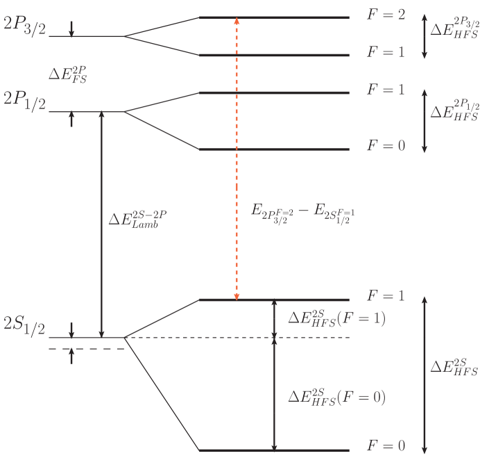
Figure 1: The 2S and 2P energy levels of muonic hydrogen.

$$\Delta E_{Lamb}^{2S-2P} = \Delta E_{ovp}+\Delta E_{KS}+\Delta E_{SE}+\Delta E_{QCD}-5.2262r_{p}^{2}+0.0347r_{p}^{3}$$

$$\Delta E_{HFS}^{2S} = \Delta E^{2S,B}_{HFS}+\Delta E^{2S,AMM}_{HFS}+\Delta E^{2S,other}_{HFS}$$

$$\Delta E_{HFS}^{2P_{3/2}} = \Delta E^{2P_{3/2},B}_{HFS}+\Delta E^{2P_{3/2},AMM}_{HFS}+\Delta E^{2P_{3/2},other}_{HFS}$$

$$\Delta E_{FS}^{2P} = \Delta E^{2P,B}_{FS}+\Delta E^{2P,AMM}_{FS}+\Delta E^{2P,other}_{FS}$$ (4)

where $\Delta E_{ovp}$ ($205.0074$ meV by the first order perturbative theory (^1stPT) and $0.1509$ meV by the second order perturbative theory), $\Delta E_{KS}$ ($1.5081$ meV) and $\Delta E_{SE}$ ($-0.6677$ meV) are the energy shifts due to the one-loop vacuum polarization, two-loop vacuum polarization and the sum of self-energy and muonic-vacuum polarization, correspondingly, $\Delta E_{QED}$ ($0.0586$ meV) is the energy shift due to all further QED corrections, and the last two terms in $\Delta E_{Lamb}^{2S-2P}$ are relevant radius-dependent contributionsannals326_500 , $\Delta E^{2S,B}_{HFS}$ ($22.8054$ meV), $\Delta E^{2P_{3/2},B}_{HFS}$ ($3.392112$ meV) and $\Delta E^{2P,B}_{FS}$ ($8.329150$ meV) are the Fermi energies, $\Delta E^{2S,AMM}_{HFS}$ ($0.0266$ meV), $\Delta E^{2P_{3/2},AMM}_{HFS}$ ($-0.000886$ meV) and $\Delta E^{2P,AMM}_{FS}$ ($0.017637$ meV) are the contributions from the anomalous magnetic moment of muon, $\Delta E^{2S,other}_{HFS}$ , $\Delta E^{2P_{3/2},other}_{HFS}$ and $\Delta E^{2P_{3/2},other}_{FS}$ are the other contributionsMartynenko2005 ; Martynenko2008 .

Some of the above perturbative results have been checked by the nonperturbative numerical (NPnum) calculations, for example within the framework of the multiconfiguration Dirac-Fock (MCDF) method in Indelicato2013 and shotting-like method using quad-precision Fortran in Carroll2011 . In this work, by using the Mathematica, we present another high precise NPnum calculations (much more precise than the quad-precision) on the energy shifts $E^{2S,B+AMM}_{HFS}$, $E^{2P_{3/2},B+AMM}_{HFS}$ and $E^{2P,B+AMM}_{FS}$ with considering the effects from the proton structure. And as a comparison, also the calculation of $\delta E_{ovp}$ is presented.

II Formula and numerical method

The leading order contribution to the fine and hyperfine structure of muonic hydrogen due to the proton structure is from the two photon exchange diagrams. Since there is IR divergence in these diagrams and such IR divergence is not dependent on the proton structure (only dependent on its charge), the one photon exchange diagram should be considered together in some way to cancel such IR divergence. This leads to the complexity in the discussion of the numerical calculation, so at present we take the effective potential from the one photon exchange diagram as an example to discuss the difference between the ^1stPT calculation and the NPnum calculation.

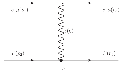
Figure 2: One photon exchange Feynman diagram considering the form factors of proton.

The Feynman diagram for one photon exchange with the proton structure is showed as Fig. 2, where the vertex of $\gamma NN$ is taken as

$$\Gamma_{\mu} = ie(F_{1}\gamma_{\mu}+\frac{iF_{2}}{2m_{p}}\sigma_{\mu\nu}q^{\nu}),$$ (5)

with $F_{1}=(G_{E}+\tau G_{M})/(1+\tau)$,$F_{2}=(G_{M}-G_{E})/(1-\tau)$, $\tau=Q^{2}/4m_{p}^{2}$, $G_{E,M}$ the electromagnetic form factors of proton, $m_{p}$ the mass of proton, and $q=p_{3}-p_{1}$ the four momentum of exchanged photon. The correction to the Coulomb potential from this diagram was discussed in the recent work Pascalutsa2015 , and in this work, we discuss its corrections to the fine and hypefine Breit potential by a precise numerical method. By using the quasipotential method the Breit potential can be expressed as annals326_500 ; Kelkar2012 .

$$V_{ovp}(r) = -\frac{\alpha^{2}}{\pi r}\int_{1}^{\infty}due^{-2um_{e}r}\frac{\sqrt{(u^{2}-1)}(2u^{2}+1)}{3u^{4}},$$

$$V_{fs}(r) = \frac{\alpha}{2m_{\mu}^{2}}[(1+2\kappa_{\mu})+\frac{2m_{\mu}}{m_{p}}(1+\kappa_{\mu})](\frac{1}{r^{3}}+\frac{G_{fs}}{r^{3}}){\bf L}\cdot{\bf S_{\mu}},$$

$$V_{HFS}^{Swave}(r) = \frac{\alpha\mu_{p}\mu_{\mu}}{4r^{3}m_{\mu}m_{p}}{\bm{\sigma}}_{\mu}\cdot{\bm{\sigma}}_{p}\frac{m^{3}r^{3}}{3}e^{-mr},$$

$$V_{HFS}^{Pwave}(r) = \frac{\alpha\mu_{p}\mu_{\mu}}{4r^{3}m_{\mu}m_{p}}[(3{\bm{\sigma}}_{\mu}\cdot{\bm{\hat{r}}}{\bm{\sigma}}_{p}\cdot{\bm{\hat{r}}}(1+h_{1})-{\bm{\sigma}}_{\mu}\cdot{\bm{\sigma}}_{p}(1+h_{2}))$$ (6)

$$+2{\bf L}\cdot{\bm{\sigma}}_{p}(\frac{1+h_{3}}{\mu_{\mu}}+\frac{m_{\mu}}{2m_{p}}\frac{h_{4}}{\mu_{p}\mu_{\mu}})],$$

where the One-loop Uehling potential $V_{ovp}$ is also presented for comparison and

$$G_{fs} = -(1+\frac{\kappa_{p}}{(1-k^{2})^{2}})e^{-mr}(1+mr)-(1+\frac{\kappa_{p}}{1-k^{2}})\frac{m^{2}}{2}r^{2}e^{-mr}$$

$$+\frac{\kappa_{p}}{(1-k^{2})^{2}}e^{-mkr}(1+mkr),$$

$$h_{1}=-e^{-mr}(1+mr)-\frac{m^{2}r^{2}}{2}e^{-mr}-\frac{m^{3}r^{3}}{6}e^{-mr},$$

$$h_{2}=-e^{-mr}(1+mr)-\frac{m^{2}r^{2}}{2}e^{-mr}-\frac{m^{3}r^{3}}{2}e^{-mr},$$

$$h_{3}=-e^{-mr}(1+mr)-\frac{m^{2}r^{2}}{2}e^{-mr},$$

$$h_{4} = (1+2\kappa_{p})(1+h_{3})+\frac{\kappa_{p}}{(1-k^{2})^{2}}e^{-mr}(1+mr)+$$

$$\frac{\kappa_{p}}{1-k^{2}}\frac{m^{2}r^{2}}{2}e^{-mr}-\frac{\kappa_{p}}{(1-k^{2})^{2}}e^{-mkr}(1+mkr),$$

with $\alpha$ the fine-structure constant, $\mu_{p}$ and $\mu_{\mu}$ the anomalous magnetic moments of proton and muon, $m$ the parameter in the electromagnetic form factors of proton which can be related with proton size as $r_{p}^{2}=12/m^{2}$, $k=2m_{p}/m$, $m_{e}$, $m_{\mu}$ the mass of electron and muon. To include the effects from the proton structure in the above Breit potential, the electromagnetic form factors of proton $G_{E,M}(Q^{2})$ have been taken approximately as the usual dipole form as Kelkar2012

$$G_{E}(Q^{2})=G_{M}(Q^{2})/\mu_{p}=1/(1+Q^{2}/m^{2})^{2},$$ (7)

with $Q^{2}=-q^{2}$. The contributions of spin related operators in the Breit potential to the $2S$ and $2P$ states are listed in Tab. 1.

	$3({\bm{\sigma}}_{\mu}\cdot{\hat{\bf r}})({\bm{\sigma}}_{p}\cdot{\hat{\bf r}})$	${\bm{\sigma}}_{p}\cdot{\bm{\sigma}}_{\mu}$	$2{\bf L}\cdot{{\bm{\sigma}}_{p}}$
$2S_{1/2}^{F=0}$	$-3$	$-3$	$0$
$2S_{1/2}^{F=1}$	$1$	$1$	$0$
$2P_{1/2}^{F=0}$	$-3$	$1$	$-4$
$2P_{1/2}^{F=1}$	$1$	$-\frac{1}{3}$	$\frac{4}{3}$
$2P_{3/2}^{F=2}$	$\frac{3}{5}$	$1$	$2$
$2P_{3/2}^{F=1}$	$-1$	$-\frac{5}{3}$	$-\frac{10}{3}$

Table 1: The contributions of the spin related operators to $2S$ and $2P$ states.

When the effects from the proton structure are neglected in the above effective potentials (taking $m\rightarrow\infty$), the energy shifts by ^1stPT reproduce the same $E^{2S,B+AMM}_{HFS}$, $E^{2P_{3/2},B+AMM}_{HFS}$ and $E^{2P,B+AMM}_{FS}$ with those used in the literaturesMartynenko2005 ; Martynenko2008 . The corrections from the proton structure in the above Breit potential is corresponding to replace the zero momentum transfer approximation by including the full $q^{2}$ dependence of the electromagnetic form factors of proton in the one photon exchange Feynman diagram. This is different with the corrections from the two photon exchange diagrams discussed in Martynenko2005 ; Martynenko2008 . Since in this work our focus is on the difference between the results by ^1stPT and NPnum calculation, we take the Breit potential as an example to show the difference.

In our numerical calculation, we use the shotting method to find out the energy spectrum by solving the reduced Schrodinger equations for $u(r)$ directly, with $u(r)=R(r)r$, $\psi({\bf r})=R(r)Y(\theta,\phi)$ and $\psi({\bf r})$ the wave function. In the detail, for muonic hydrogen we take approximately $u(r=0)\approx u(r=10^{-50}fm)$ and $u(r=\infty)\approx u(r=10^{6}{fm})$ to simulate the behaviors of wave function at the boundary. We keep 200 digits of the numbers in the calculation and take the PrecisionGoal of NDSolve in Mathematica as 15, respectively. By these approximations, as a check we reproduce the energy spectrum of muonic hydrogen under the Coulomb potential with the precision better than $10^{-10}$ meV. Since the numerical calculation is based on the shotting method, the precision is not sensitive on the form of the potentials or the solutions, this is different with the basis expansion method or variational methods usually used, and ensures our numerical calculation reliable for the other potentials.

III numerical result

In Tab. 2 and 3, we present the results by the ^1stPT and NPnum calculation including the effects from the proton structure in the Breit potential. The corresponding results without considering the proton structure by ^1stPT and from the one-loop Uehling potential are also presented for comparison.

$r_{p}$(fm)	$\Delta E_{FS}^{2P}$		$\Delta E_{HFS}^{2P^{3/2}}$		$\Delta E_{ovp}$
	1stPT	NPnum	1stPT	NPnum	1stPT	NPnum
0	8.34676	-	3.39121	-	205.00659	205.15747
0.83112	8.34673	8.34703	3.39121	3.39123	205.00659	205.15747
0.84184	8.34672	8.34702	3.39121	3.39123	205.00659	205.15747
0.87800	8.34672	8.34702	3.39121	3.39123	205.00659	205.15747

Table 2: Energy shifts of different potentials using perturbative and precise numerical calculations in meV where ^1stPT and NPnum denote the first order pertubative and precise nonperturbative numerical calculation, respectively. The typical proton size $r_{p}=0,0.83112,0.84184,0.878fm$ are taken as examples for comparison. The results by ^1stPT are same with those in annals326_500 ; Martynenko2005 .

$r_{p}$(fm)	$\Delta E_{HFS}^{2S}(F=1)$		$\Delta E_{HFS}^{2S}(F=0)$		$\frac{\Delta E_{HFS}^{2S}(F=0)}{\Delta E_{HFS}^{2S}(F=1)}$		$\Delta E_{HFS}^{2S}$
	1stPT	NPnum	1stPT	NPnum	1stPT	NPnum	1stPT	NPnum
0	5.70798	-	17.12394	-	3	-	22.83192	-
0.83112	5.67921	5.66943	17.03762	17.12628	3	3.0208	22.71683	22.79571
0.84184	5.67884	5.66918	17.03651	17.12406	3	3.0206	22.71535	22.79324
0.87800	5.67759	5.66832	17.03277	17.11676	3	3.0197	22.71036	22.78508

Table 3: Energy shifts of different potentials using perturbative and precise numerical calculations in meV. The notations are same with Tab. 2. The results by ^1stPT are same with those in Martynenko2008 .

From the last two columns of Tab. 2, we see the results by ^1stPT and NPnum calculations give about $0.15088$ meV difference for $V_{ovp}$. Actually the second order perturbative calculation of $V_{ovp}$ gives the contribution about $0.1509$ meV annals326_500 , so the combination of the first and second order pertubative calculation of $V_{ovp}$ is almost same with our NPnum calculation. When including the effects from the proton structure and taking $r_{p}=0.83112$ fm, $0.84184$ fm, $0.878$ fm as examples, the differences between the ^1stPT and precise NPnum calculations are about $3\times 10^{-4}$ and $2\times 10^{-5}$ meV for the fine and hyperfine splitting of $2P$ states, respectively, and also these two splittings are almost independent on the proton size in the region $r_{p}\in[8.2,9.0]$ fm. From the Tab. 3, we see the derivations of the ^1stPT and NPnum calculation are about $-0.009$ and $0.02$ meV for the hyperfine splitting of $2S$ state $\Delta E_{HFS}^{2S}(F=1)$ and $\frac{1}{4}\Delta E_{HFS}^{2S}$, respectively, which should not be omitted comparing with the precision of current experiments. We want to emphasize that by the NPnum calculation, the ratios $\frac{\Delta E_{HFS}^{2S}(F=0)}{\Delta E_{HFS}^{2S}(F=1)}$ are not strictly equal to $3$ as predicted by the ^1stPT, but are about $3.02$ as showed in Tab. 3 and the absolute difference between $\Delta E_{HFS}^{2S}(F=1)$ and $\frac{1}{4}\Delta E_{HFS}^{2S}$ are large. Such a discrepancy means the relation $\Delta E_{HFS}^{2S}(F=1)=\frac{1}{4}\Delta E_{HFS}^{2S}$ is not suitable to be used as usual. To show the results in a more direct way, we use the polynome of $r_{p}$ to fit the numerical results of $\Delta E_{HFS}^{2S}(F=1)$ in the region $r_{p}\in[8.2,9.0]$ fm by taking one point every $0.001$ fm and the results are expressed as

$$\Delta E_{HFS}^{2S}(F=1,\textrm{NPnum}) = 5.68008-0.00261343r_{p}-0.0122699r_{p}^{2}~{}~{}~{}~{}~{}~{}~{}\textrm{meV}$$

$$\Delta E_{HFS}^{2S}(F=1,^{1st}\textrm{PT}) = 5.70793-0.0346149r_{p}+0.0000613066r_{p}~{}~{}~{}~{}\textrm{meV}$$ (8)

with the residual mean square of the fitting as small as about $10^{-11}$ meV².

After including the difference of $\Delta E_{HFS}^{2S}(F=1)$ by our estimation, the theoretical energy shift Eq.(1) is changed as

$$E_{2P_{3/2}^{F=2}}^{Th}-E_{2S_{1/2}^{F=1}}^{Th} = 209.9869-5.2262r_{p}^{2}+0.0347r_{p}^{3}$$ (9)

and if $r_{p}$ is taken as $0.878$fm, then the modified $E_{2P_{3/2}^{F=2}}^{Th}-E_{2S_{1/2}^{F=1}}^{Th}$ is estimated as $205.9816$ meV, which deviates from the experimental results about $0.31$ meV. This means after using the precise NPnum calculation of $\Delta E_{HFS}^{2S}(F=1)$, the discrepancy of the measurement of the proton size is reduced about 3%, while if we take the $\frac{1}{4}\Delta E_{HFS}^{2S}$ as input then the energy shift Eq.(1) is changed as

$$E_{2P_{3/2}^{F=2}}^{Th}-E_{2S_{1/2}^{F=1}}^{Th} = 209.9579-5.2262r_{p}^{2}+0.0347r_{p}^{3}$$ (10)

and if $r_{p}$ is taken as $0.878$fm, then $E_{2P_{3/2}^{F=2}}^{Th}-E_{2S_{1/2}^{F=1}}^{Th}$ is estimated as $205.9526$ meV, which deviates from the experimental results about $0.34$ meV. We see the discrepancy will be intensified about 7%. The full results show we should be careful to deal with the splitting beyond the ^1stPT and should replace $\frac{1}{4}\Delta E_{HFS}^{2S}$ by $\Delta E_{HFS}^{2S}(F=1)$ in the calculation.

According to Tab. 1 and Fig. 1, we also have

$$E_{2P_{3/2}^{F=1}}-E_{2S_{1/2}^{F=0}}=\Delta E_{Lamb}^{2S-2P}-\frac{5}{8}\Delta E_{HFS}^{2P_{3/2}}+\Delta E_{FS}^{2P}+\frac{3}{4}\Delta E_{HFS}^{2S},$$ (11)

and

$$\Delta E=(E_{2P_{3/2}^{F=1}}-E_{2S_{1/2}^{F=0}})-(E_{2P_{3/2}^{F=2}}-E_{2S_{1/2}^{F=1}})=\Delta E_{HFS}^{2S}-\Delta E_{HFS}^{2P_{3/2}}.$$ (12)

We note that $\Delta E$ depends on $\Delta E_{HFS}^{2S}$ instead of $\Delta E_{HFS}^{2S}(F=1)$ appeared in $E_{2P_{3/2}^{F=2}}-E_{2S_{1/2}^{F=1}}$, so for $\Delta E$ the NPnum calculation gives relative larger corrections. We present the results of $\Delta E$ from the Breit potential by the two methods in Tab. 4. With the different proton radius as input, the differences of $\Delta E$ are about $10^{-3}\sim 10^{-2}$ meV. At present, the $E_{2P_{3/2}^{F=2}}-E_{2S_{1/2}^{F=1}}$ and $E_{2P_{3/2}^{F=1}}-E_{2S_{1/2}^{F=0}}$ transition frequency in muonic hydrogen have been both measured with very high accuracy science339_417 , the experimental value of $\Delta E$ is about $19.56$ meV. Our numerical results are different from the experimental value since we have not considered the other corrections beside Breit potential. However, our calculation implies the precise NPnum calculation is needed.

$r_{p}$(fm)	$\Delta E(\textrm{meV})$
	1stPT	NPnum
0	$19.44070$	-
0.83112	$19.32562$	$19.40434$
0.84184	$19.32414$	$19.40187$
0.87800	$19.31915$	$19.39371$

Table 4: The difference of $2S-2P$ transition energy $\Delta E$ of muonic hydrogen in meV with different radius of proton as input. The notations are same with Tab. 2.

Since the obvious difference exists between the ^1stPT and precise NPnum calculations of the hyperfine splitting of muonic hydrogen’s $2S$ state, we also present the similar comparison of the $ep$ system in Tab. 5 where the results show the calculation for the hyperfine splitting of $S$ state in $ep$ system by the ^1stPT is also not good enough. Different with ^1stPT, the results by the precise NPnum method are more sensitive on the proton size.

$r_{p}$(fm)	$E_{HFS}^{1S}(kHz)$		$E_{HFS}^{2S}(kHz)$
	1stPT	NPnum	1stPT	NPnum
0	$1420478.8$	-	$177559.8$	-
0.83112	$1420440.1$	$1425769.6$	$177555.0$	$178221.2$
0.84184	$1420439.6$	$1425700.8$	$177555.0$	$178212.6$
0.87800	$1420438.0$	$1425481.1$	$177554.7$	$178185.1$

Table 5: Frequencies in kHz of hyperfine splitting $E_{HFS}^{1S}$ and $E_{HFS}^{2S}$ in hydrogen.

In a summary, by using shotting method in Mathematica we give a very high precise NPnum calculation for the energy shifts of the Breit potential including the effects from the proton structure. Our results show that when taking into account the proton structure, the precise NPnum calculations give very small corrections to the hyperfine splitting of $2P_{3/2}$ and fine structure of $2P$ states, but give about $-0.009$ meV and $0.08$ meV differences for the hyperfine splitting $\Delta E_{HFS}^{2S}(F=1)$ and $\Delta E_{HFS}^{2S}$ of munoic hydrogen with those usually used in the literatures by ^1stPT. The similar properties are also found in the hydrogen case.

IV Acknowledgments

This work is supported by the National Sciences Foundations of China under Grant No. 11375044 and in part by the Fundamental Research Funds for the Central Universities under Grant No. 2242014R30012.

References

• (1) Pohl R, et al., Nature 466, 213 (2010).
• (2) Aldo Antognini, et al., Science 339, 417 (2013).
• (3) Mohr P J, Taylor B N, Newell D B , Rev. Mod. Phys. 84, 1527 (2012).
• (4) Sarely G. Karshenboim, Phys. Rep. 422, 1 (2005).
• (5) E. Borie, Annas of Physics 327, 733 (2012).
• (6) C. Adamuscin, S. Dubnicka, and A. Z. Dubnickova, Prog. Part. Nucl. Phys. 67, 479 (2012); I. Sick, Prog. Part. Nucl. Phys. 67, 473 (2012).
• (7) Jean-Philippe Karr, Laurent Hilico, Phys. Rev. Lett. 109, 103401 (2012).
• (8) Vernon Barger, Cheng-Wei Chiang, Wai-Yee Keung, Danny Marfatia, Phys. Rev. Lett. 106, 153001 (2011).
• (9) Savely G. Karshenboim, Phys. Rev. D 90, 053012 (2014).
• (10) Ashot Gasparian, EPJ Web Conf. 73, 07006 (2014).
• (11) R. N. Faustov, A. P. Martynenko, Teor. Math. Phys. 64, 765 (1985); R. N. Faustov, A. P. Martynenko, JETP 88, 672 (1999).
• (12) U. D. Jentschura, Annals. Phys. 326, 500 (2011).
• (13) A. P. Martynenko, Phys. Rev. A 71, 022506 (2005).
• (14) A. P. Martynenko, Phys. Atomic Nuclei. 71, 125 (2008).
• (15) P. Indelicato, Phys. Rev. A 87, 022501 (2013).
• (16) J. D. Carroll, A. W. Thomas, J. Rafelski, G. A. Miller, Phys. Rev. A 84, 012506 (2011).
• (17) Franziska Hagelstein, Vladimir Pascalutsa, Phys. Rev. A 91,040502(2015)(R).
• (18) N.G.Kelkar, F. Garcfa Daza, M. Nowakowski, Nucl. Phys. B 864, 382(2012).