Topologically non-trivial Floquet band structure in a system undergoing photonic transitions in the ultra-strong coupling regime

Abstract

We consider a system of dynamically-modulated photonic resonator lattice undergoing photonic transition, and show that in the ultra-strong coupling regime such a lattice can exhibit non-trivial topological properties, including topologically non-trivial band gaps, and the associated topologically-robust one-way edge states. Compared with the same system operating in the regime where the rotating wave approximation is valid, operating the system in the ultra-strong coupling regime results in one-way edge modes that has a larger bandwidth, and is less susceptible to loss. Also, in the ultra-strong coupling regime, the system undergoes a topological insulator-to-metal phase transition as one varies the modulation strength. This phase transition has no counter part in systems satisfying the rotating wave approximation, and its nature is directly related to the non-trivial topology of the quasi-energy space.

Creating topological effects klitzing80 for both electrons qi11 and photons lu14 ; haldane08 ; raghu08 ; wang09 ; hafezi11 ; poo11 ; hafezi13 ; khanikaev13 ; longhi13 ; liang13 ; mittal14 ; li14 ; slobozhanyuk15 are of significant current interests. A powerful mechanism for achieving non-trivial topology in a system is to dynamically modulate the system in time. For electrons, such modulation can be achieved by coupling with an external electromagnetic field, and has been used to create an electronic Floquet topological insulator kitagawa10 ; inoue10 ; lindner11 ; leon13 ; rudner13 ; cayssol13 . For photons, optical analogue of Floquet topological insulators has been demonstrated rechstman13 . Also, time-dependent refractive-index modulations can be used to create an effective magnetic field fang12np , which can break time-reversal symmetry and create a one-way edge state that is topologically protected against arbitrary disorders.

All previous works on the topological behaviors of dynamically modulated systems have considered only the weak-coupling regime where the modulation strength is far less than the modulation frequency, and applied the rotating wave approximation (RWA). On the other hand, in recent years, the study of light-matter interactions in the ultra-strong coupling regime, where the rotating wave approximation is no longer valid, is becoming important irish05 ; irish07 ; rabl11 ; schiro12 ; burillo14 ; gunter09 ; imamoglu09 ; niemczyk10 . It is therefore of fundamental importance to understand topological effects beyond the rotating wave approximation.

In this Letter, we analyze a time-dependent Hamiltonian first proposed in Ref. fang12np for achieving an effective magnetic field for photons. Unlike Ref. fang12np , however, here we focus the ultra-strong coupling regime where the rotating wave approximation is no longer valid. Experimentally, reaching such ultra-strong coupling regime is in fact relatively straightforward with current photonic technology tzuang14 . For this system in the ultra-strong coupling regime, we show that the topologically protected one-way photonic edge states can persist over a broad parameter range. Compared with the weak-coupling regime, the topologically protected one-way edge state is less susceptible to intrinsic losses. We also show that, as one varies the modulation strength, there is a topological phase transition that is uniquely associated with the ultra-strong coupling regime, and has no counter part in weak-coupling systems.

We start with the Hamiltonian fang12np

$$H=\omega_{A}\sum_{m}a^{\dagger}_{m}a_{m}+\omega_{B}\sum_{n}b^{\dagger}_{n}b_{n}+\sum_{\langle mn\rangle}V\cos(\Omega t+\phi_{mn})(a^{\dagger}_{m}b_{n}+b^{\dagger}_{n}a_{m}),$$ (1)

which describes a lattice of photonic resonators as shown in Figure 1. The lattice consists of two sub-lattices, each consisting of resonators of resonant frequencies $\omega_{A}$ and $\omega_{B}$, respectively. $a^{\dagger}$ ($a$) and $b^{\dagger}$ ($b$) are the creation (annihilation) operators associated with the resonators in the two sub-lattices. The coupling between the resonators are modulated dynamically, where $V$ is the maximum coupling strength, $\Omega=\omega_{A}-\omega_{B}$ is the modulation frequency, and $\phi_{mn}$ is the modulation phase. Such a modulation drives a photonic transition winn99 between nearest neighbor resonators.

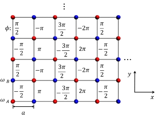
Figure 1: Lattice composed of two types of resonators $A$ (red) and $B$ (blue). The lines represent coupling (or bonds) between nearest neighbors. All coupling strengths are modulated in time harmonically. For all bonds along the horizontal direction the modulation phase is zero. The bonds along the vertical direction have a spatial distribution of modulation phases as specified in the figure. The specified phases are for the hopping matrix elements of the Hamiltonian in Eq. (1) along the positive $y$ direction.

Eq. (1) can be transformed to the rotating frame with

$$\tilde{a}_{m}(\tilde{b}_{n})=a_{m}(b_{n})e^{i\omega_{A(B)}t}.$$ (2)

The Hamiltonian then becomes

$$\tilde{H}=\frac{V}{2}\sum_{\langle mn\rangle}(\tilde{a}^{\dagger}_{m}\tilde{b}_{n}e^{-i\phi_{mn}}+\tilde{b}^{\dagger}_{n}\tilde{a}_{m}e^{i\phi_{mn}}+\tilde{a}^{\dagger}_{m}\tilde{b}_{n}e^{i2\Omega t+i\phi_{mn}}+\tilde{b}^{\dagger}_{n}\tilde{a}_{m}e^{-i2\Omega t-i\phi_{mn}}),$$ (3)

where the first two terms define the Hamiltonian $\tilde{H}_{\mathrm{RWA}}$ in the rotating wave approximation, and the last two terms are commonly referred as the counter-rotating terms.

Ref. fang12np considered the weak-coupling regime where $V\ll\Omega$ and applied the rotating wave approximation by ignoring the counter-rotating terms in Eq. (3). In this case, $\tilde{H}\simeq\tilde{H}_{\mathrm{RWA}}$ becomes time-independent, and is identical to the Hamiltonian of a quantum particle on a lattice subject to a magnetic field described by a vector potential $\bm{A}$, with $\phi_{mn}=\int_{m}^{n}\bm{A}\cdot d\bm{l}$ peierls33 . Such an effective magnetic field provides a new mechanism for controling the propagation of light fang13 ; fang13oe ; lin14 ; yuan15 . In particular, it can be used to achieve a topologically protected one-way edge state fang12np .

However, from an experimental point of view, it is important to explore the topological behavior of the Hamiltonian of Eq. (1) beyond the weak-coupling regime. The required modulation in Eq. (1) can be achieved electro-optically tzuang14 , in which case $V\sim\delta n/n\cdot\omega_{0}$, where $n$ is the refractive index, $\delta n$ is the strength of the index modulation, and $\omega_{0}$ is the operating frequency. For electro-optic modulation of silicon, to minimize free-carrier loss, $\delta n/n\approx 10^{-5}-10^{-4}$ lipson05 . Optical communication typically uses an $\omega_{0}$ corresponding to a free-space wavelength near 1.5 micron. Thus $V$ is typically between 10-100 GHz. On the other hand, the modulation frequency $\Omega$ in electro-optic modulation is also on the order of 10-100 GHz tzuang14 . Thus, experimentally one can readily operate in the regime with $V\sim\Omega$. Similar conclusion can be reached for the acoustic-optical modulation scheme implemented in Ref. li14 for achieving a photonic gauge potential. Unlike the electronic transition, where reaching the ultra-strong coupling regime is a significant challenge scalari12 ; geiser12 ; li13 ; scalari14 , for photonic transition winn99 it is in fact rather natural that the system operates in the ultra-strong coupling regime. Thus, systems exhibiting photonic transition can be readily used to explore the physics of ultra-strong coupling.

To explore the topological properties of Eq. (1) in the ultra-strong coupling regime, we perform a Floquet analysis of the Hamiltonian of Eq. (3). Here we choose a spatial distribution of the modulation phase as shown in Figure 1. All bonds along the horizontal direction have a zero modulation phase. The bonds along the vertical direction have a spatial distribution of modulation phases. In the weak-coupling regime, such a distribution corresponds to an effective magnetic flux of $\pi/2$, or 1/4 of the magnetic flux quanta per unit cell. The system is therefore topologically non-trivial in the weak-coupling regime. The aim of the Floquet analysis is then to see to what extent such non-trivial topological feature persist as one goes beyond the rotating wave approximation.

Our Floquet band structure analysis follows that of Refs. shirley65 ; samba73 . The system in Figure 1 is periodic spatially. Therefore the Hamiltonian can be written in the wavevector space ($\bm{k}$-space). For each $\bm{k}$ point, $\tilde{H}$ in Eq. (3) has a period in time $T=\pi/\Omega$. Therefore, the solution of the equation $id/dt|\Psi\rangle-\tilde{H}|\Psi\rangle=0$ in general takes the form $|\Psi\rangle=e^{-i\varepsilon t}|\Phi\rangle$, where $|\Phi(t+T)\rangle=|\Phi(t)\rangle$ has a periodicity $T$ in time, and is commonly referred to as the Floquet eigenstate. $\varepsilon$ is the quasi-energy and is defined in the temporal first Brillouin zone $\varepsilon\in[-\pi/T,\pi/T]=[-\Omega,\Omega]$. The quasi-energies and the Floquet eigenstates can be obtained by solving numerically the eigenvalue equation: $(\tilde{H}-i\partial/\partial t)|\Phi\rangle=\varepsilon|\Phi\rangle$ shirley65 ; samba73 . The quasi energy thus obtained as a function of $\bm{k}$ defines the Floquet band structure.

As an important subtlety, when performing numerical calculation of the Floquet band structures, it is essential to perform a gauge transformation such that the resulting Hamiltonian has the smallest possible temporal period. For our case here, the transformation of Eq. (2), which is a gauge transformation, serves this purpose. While the Hamiltonians $H$ (in Eq. (1)) and $\tilde{H}$ (in Eq. (3)) are equivalent to each other since they are related by the gauge transformation of Eq. (2), the temporal periods of $H$ and $\tilde{H}$ are $2\pi/\Omega$ and $\pi/\Omega$, respectively. A key aspect of topological band structure analysis is to identify band gaps that are topologically non-trivial. On the other hand, if one analyze $H$ directly, since the corresponding temporal first Brillouin zone is smaller, there is additional band folding along the quasi-energy axis, which obscures the band gap. The use of $\tilde{H}$ in Eq. (3) is in fact quite important for the analysis of the topological aspects of the Floquet band structure.

We now examine the Floquet band structure of the system. $\tilde{H}$ has a spatial periodicity of 4$a$ by 2$a$ along the $x$ and $y$ directions, respectively. Thus, its Floquet band structure has 8 bands, as we can see in Figure 2.

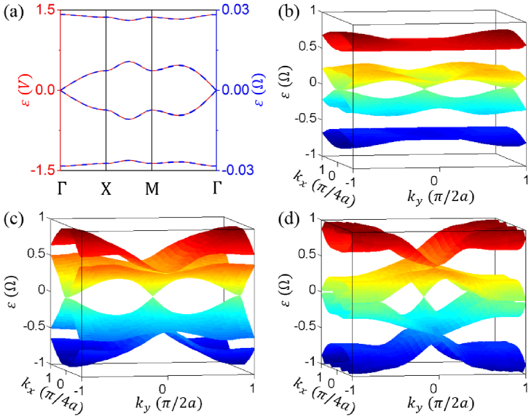
Figure 2: Floquet band structure for the Hamiltonian $\tilde{H}$ of Eq. (3), (a) with RWA from $\tilde{H}_{\mathrm{RWA}}$ (red solid line) and $V=0.02\Omega$ (blue dashed line), (b) $V=0.5\Omega$, (c) $V=1.1\Omega$, and (d) $V=1.5\Omega$.

As a comparison, we first consider the band structure of the Hamiltonian $\tilde{H}_{\mathrm{RWA}}$ as defined by ignoring the counter-rotating terms in Eq. (3). $\tilde{H}_{\mathrm{RWA}}$ has a spatial periodicity of 4$a$ by 1$a$ along the $x$ and $y$ directions, respectively. However, to facilitate the comparison with the band structure of $\tilde{H}$, here we plot the bandstructure of $\tilde{H}_{\mathrm{RWA}}$ with the spatial periodicity of 4$a$ by 2$a$ as well. The resulting RWA band structure, as shown in Figure 2a, thus contains 8 bands. The bands are two fold degenerate. The bandstructure has the same shape for different values of $V$. (Figure 2a).

In the RWA band structure, there are two gaps separating the middle group of four bands from the upper and the lower groups, each of two bands, respectively. These gaps are topologically non-trivial, as can be checked by calculating the Chern number rudner13 :

$$\mathcal{C}=-\frac{1}{2\pi}\sum_{\alpha}\int dk_{x}dk_{y}(\nabla_{\vec{k}}\times\mathcal{A}_{\alpha}),$$ (4)

where the summation is over the group of bands, each band indiced by a different $\alpha$.

$$\mathcal{A}_{\alpha}=\langle\Phi_{\alpha}(\vec{k},t)|i\nabla_{\vec{k}}|\Phi_{\alpha}(\vec{k},t)\rangle,$$ (5)

The Chern numbers for the upper, middle and lower groups of bands are +1, -2, +1, respectively. (As a side note, the middle group of four bands can actually be separated into two subgroups each consisting of two bands, separated by Dirac points at $\varepsilon=0$. Each of the subgroup has a Chern number -1.) The topological analysis here is consistent with the association of an effective magnetic field in this system. The gaps remain open for all non-zero values of $V$. Thus with the rotating wave approximation there is no phase transition as one varies $V$.

Having reviewed the band structure of $\tilde{H}_{\mathrm{RWA}}$, we now consider the Floquet band structure of the full Hamiltonian $\tilde{H}$. Figure 2a shows the cases of $V=0.02\Omega$, the Floquet band structure $\tilde{H}$ agrees very well with that of the $\tilde{H}_{\mathrm{RWA}}$.

As one increases $V$ to approximately $V>0.1\Omega$, the RWA is no longer adequate to describe the band structure of $\tilde{H}$. Hence, it is no longer possible to interpret the bandstructure using the concept of an effective magnetic field. Nevertheless, the two gaps remain open for $V$ ranging from near zero to $1.1\Omega$ (see Figures 2). Therefore, in this range of $V$, the Chern numbers for the upper, middle and lower groups of bands must remain unchanged at +1, -2, +1, respectively, and hence the topological aspects of the band structure remains the same as one goes into the ultra-strong coupling regime.

As $V$ increases from 0, the bands gradually move away from $\varepsilon=0$, and start to occupies more of the temporal first Brillouin zone (See Figure 2b). At $V\sim\Omega$, some of these bands reach the edge of the temporal first Brillouin zone. Further increase of $V$ then results in the folding back of these bands back into the temporal first Brillouin zone and the closing of the gaps as we see in Figure 2c with $V=1.1\Omega$. No gap is found for larger values of $V$. We see that the increase of $V$ induces a topological phase transition: the system behaves as a Floquet topological insulator at small $V$, and a gapless and topologically trivial “metal” at large $V$.

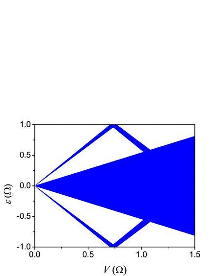
Figure 3: The projected RWA band structure folded into the temporal first Brillouin zone as a function of $V$. The blue regions correspond to the bands. The white regions are the band gap regions.

The values of $V$ required for achieving such a topological phase transition can be estimated by folding the RWA band structure into the temporal first Brillouin zone of [$-\Omega$, $\Omega$] (Figure 3), which predicts that the gap closes at $V=1.1\Omega$. In comparsion, for the full Hamilontian of Eq. (3), the gap actually closes at $V=1.11\Omega$. Therefore, We see that this topological phase transition is directly related to the non-trivial topology of the quasi-energy space.

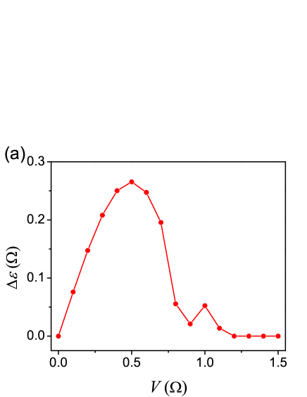
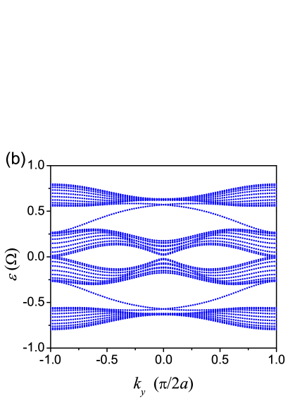
Figure 4: (a) The bandwidth of the topologically non-trivial gap as a function of $V$. (b) The projected bandstructure at $V=0.5\Omega$.

A key signature of a topologically non-trivial band gap is the existence of a one-way edge state in a strip geometry. We therefore calculate the projected Floquet band structure for a strip that is infinite in the $y$-direction and has a width of $21a$ in the $x$-direction. The projected band structure consists of the quasi energy of all the eigenstates of the system as a function of $k_{y}$. The projected band consists of three groups of bands separated by two topologically non-trivial band gaps. We observe the existence of one-way edge mode that spans these topologically non-trivial band gaps, as shown in Figure 4b with $V=0.5\Omega$. Thus the one-way edge state persist in the ultra-strong coupling regime.

For applications of one-way edge modes to carry information, optimizing the bandwidth of such a one-wage edge mode is important. Since the one-way edge mode spans the topologically non-trivial band gap, the size of such a gap becomes a good measure of the bandwidth of the one-way edge mode. In Figure 4a, we plot the size of the topologically non-trivial band gap, as a function of modulation strength $V$. The bandwidth increases with $V$ for small $V$, peaks at $V=0.5\Omega$, and then decreases to zero signifying the topological phase transition mentioned above. For a given modulation frequency $\Omega$ therefore, the bandwidth of the one-way edge mode maximizes at the ultra-strong coupling regime.

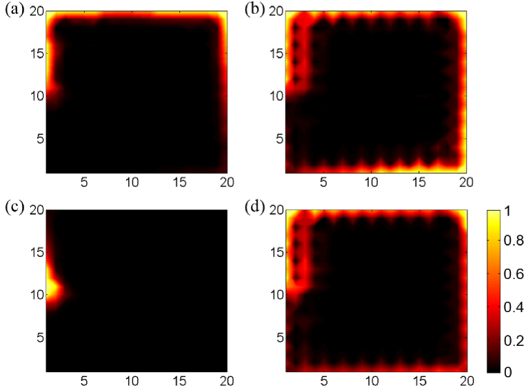
Figure 5: The simulation results with the Hamiltonian (1) in a $20\times 20$ resonator lattice ($\omega_{A}=12\pi c/a$, $\omega_{B}=0$). A point source is placed at the location (1,10). The propagation field profiles are plotted at time (a) $t=100a/c$ with $V=0.02\Omega$ and the source frequency $\omega_{s}=V$; (b) $t=10a/c$ with $V=0.5\Omega$ and $\omega_{s}=V$; (c) same as (a) and (d) same as (b) with a loss coefficient $\gamma=0.1c/a$ at steady state.

The one-way edge mode is topologically robust against disorder-induced back-scattering. However, such a mode is still susceptible to intrinsic losses of the materials. For practical application then mitigation of the effect of intrinsic loss is important. For a given modulation frequency $\Omega$, operating in the ultra-strong coupling regime results in the one-way edge modes that have larger group velocities, and hence are less susceptible to loss, as compared to operating in the weak-coupling regime. As an illustration, we consider a finite structure described by the Hamiltonian of Eq. (1) of a size of $20a$ by $20a$ (Figure 5). We consider two systems in the weak-coupling and ultra-strong coupling regime, corresponding to $V=0.02\Omega$, and $V=0.5\Omega$, respectively. To probe the systems, we place a point source at the location ($1a$, $10a$), and choose the frequencies of the point source to be inside one of the topologically non-trivial band gaps. Both systems indeed support one-way edge modes as shown in Figures 5a and b. To study the effect of loss, we further include into Eq. (1) an extra term $-\gamma\left(\sum_{m}a^{\dagger}_{m}a_{m}+\sum_{n}b^{\dagger}_{n}b_{n}\right)$, where $\gamma=0.1c/a$ is the loss coefficient. The steady-state field distributions for the same source are shown in Figures 5c and d respectively. We see that the photons indeed have a much longer propagation distance in the ultra-strong coupling regime with $V=0.5\Omega$ (Figure 5d), as compared to the weak-coupling regime with $V=0.02\Omega$ (Figure 5c).

In summary, we consider a system of dynamically-modulated photonic resonator lattice undergoing photonic transition, and show that such a lattice can exhibit non-trivial topological properties in the ultra-strong coupling regime. From an experimental and practical point of view, for the same modulation frequency, operating the system in the ultra-strong coupling regime results in one-way edge modes that has a larger bandwidth, and is less susceptible to loss, as compared to operating the same system in the weak-coupling regime. Our work therefore should provide useful guidance to the experimental quest in seeking to demonstrate topological effects related to time-reversal symmetry breaking on-chip tzuang14 . We also show that in the ultra-strong coupling regime, the system undergoes a topological phase transition as one varies the modulation strength. This phase transition has no counter part in weak-coupling systems, and its nature is directly related to the non-trivial topology of the quasi-energy space. In the context of recent significant fundamental interests in exploring the ultra-strong coupling physics irish05 ; irish07 ; rabl11 ; schiro12 ; burillo14 ; gunter09 ; imamoglu09 ; niemczyk10 ; scalari12 ; geiser12 ; li13 ; scalari14 , our work points to the exciting prospect of exploring non-trivial topological effects in ultra-strong coupling regime.

- (1) K. V. Klitzing, G. Dorda, and M. Pepper, Phys. Rev. Lett. 45, 494 (1980).
- (2) X.-L Qi, and S.-C. Zhang, Rev. Mod. Phys. 83, 1057 (2011).
- (3) L. Lu, J. D. Joannopoulos, and M. Soljačić, Nat. Photonics 8, 821 (2014).
- (4) F. D. M. Haldane and S. Raghu, Phys. Rev. Lett. 100, 013904 (2008).
- (5) S. Raghu and F. D. M. Haldane, Phys. Rev. A 78, 033834 (2008).
- (6) Z. Wang, Y. Chong, J. D. Joannopoulos, M. Soljačić, Nature 461, 772 (2009).
- (7) M. Hafezi, E. A. Demler, M. D. Lukin, and J. M. Taylor, Nat. Phys. 7, 907 (2011).
- (8) Y. Poo, R. -X. Wu, Z. Lin, Y. Yang, and C. T. Chan, Phys. Rev. Lett. 106, 093903 (2011).
- (9) M. Hafezi, S. Mittal, J. Fan, A. Migdall, and J. M. Taylor, Nat. Photonics 7, 1001 (2013).
- (10) A. B. Khanikaev, S. H. Mousavi, W. -K. Tse, M. Kargarian, A. H. MacDonald, and G. Shvets, Nature Materials 12, 233 (2013).
- (11) S. Longhi, Opt. Lett. 38, 3570 (2013).
- (12) G. Q. Liang and Y. D. Chong, Phys. Rev. Lett. 110, 203904 (2013).
- (13) S. Mittal, J. Fan, A. Faez, J. M. Taylor, and M. Hafezi, Phys. Rev. Lett. 113, 087403 (2014).
- (14) E. Li, B. J. Eggleton, K. Fang, and S. Fan, Nat. Commun. 5, 3225 (2014).
- (15) A. P. Slobozhanyuk, A. N. Poddubny, A. E. Miroshnichenko, P. A. Belov, and Y. S. Kivshar, Phys. Rev. Lett. 114, 123901 (2015).
- (16) T. Kitagawa, E. Berg, M. Rudner, and E. Demler, Phys. Rev. B 82, 235114 (2010).
- (17) J. Inoue and A. Tanaka, Phys. Rev. Lett. 105, 017401 (2010).
- (18) N. H. Lindner, G. Refael, and V. Galitski, Nat. Phys. 7, 490 (2011).
- (19) A. Gómez-León and G. Platero, Phys. Rev. Lett. 110, 200403 (2013).
- (20) M. S. Rudner, N. H. Lindner, E. Berg, and M. Levin, Phys. Rev. X 3, 031005 (2013).
- (21) J. Cayssol, B. Dóra, F. Simon, and R. Moessner, Phys. Status Solidi RRL 7, 101 (2013).
- (22) M. C. Rechstman, J. M. Zeuner, Y. Plotnik, Y. Lumer, D. Podolsky, F. Dreisow, S. Nolte, M. Segev, and A. Szameit, Nature 496, 196 (2013).
- (23) K. Fang, Z. Yu, and S. Fan, Nat. Photonics 6, 782 (2012).
- (24) E. K. Irish, J. Gea-Banacloche, I. Martin, and K. C. Schwab, Phys. Rev. B 72, 195410 (2005).
- (25) E. K. Irish, Phys. Rev. Lett. 99, 173601 (2007).
- (26) P. Rabl, Phys. Rev. Lett. 107, 063601 (2011).
- (27) M. Schiró, M. Bordyuh, B. öztop, and H. E. Türeci, Phys. Rev. Lett. 109, 053601 (2012).
- (28) E. Sanchez-Burillo, D. Zueco, J. J. Garcia-Ripoll, and L. Martin-Moreno, Phys. Rev. Lett. 113, 263604 (2014).
- (29) G. Günter, A. A. Anappara, J. Hees, A. Sell, G. Biasiol, L. Sorba, S. De Liberato, C. Ciuti, A. Tredicucci, A. Leitenstorfer, and R. Huber Nature 458, 178 (2009).
- (30) A. Imamoğlu, Phys. Rev. Lett. 102, 083602 (2009).
- (31) T. Niemczyk, F. Deppe, H. Huebl, E. P. Menzel, F. Hocke, M. J. Schwarz, J. J. Garcia-Ripoll, D. Zueco, T. Hümmer, E. Solano, A. Marx, and R. Gross, Nat. Phys. 6, 772 (2010).
- (32) L. D. Tzuang, K. Fang, P. Nussenzveig, S. Fan, and M. Lipson, Nat. Photonics 8, 701 (2014).
- (33) J. N. Winn, S. Fan, J. D. Joannopoulos, and E. P. Ippen, Phys. Rev. B 59, 1551 (1999).
- (34) R. E. Peierls, Z. Phys. 80, 763 (1933).
- (35) K. Fang and S. Fan, Phys. Rev. Lett. 111, 203901 (2013).
- (36) K. Fang, Z. Yu, and S. Fan, Opt. Express 21, 18216 (2013).
- (37) Q. Lin and S. Fan, Phys. Rev. X 4, 031031 (2014).
- (38) L. Yuan and S. Fan, arXiv:1502.06037.
- (39) M. Lipson, J. Lightwave Technol. 23 4222 (2005).
- (40) G. Scalari, C. Maissen, D. Turčinková, D. Hagenmüller, S. De Liberato, C. Ciuti, C. Reichl, D. Schuh, W. Wegscheider, M. Beck, J. Faist, Science 335, 1323 (2012).
- (41) M. Geiser, F. Castellano, G. Scalari, M. Beck, L. Nevou, and J. Faist, Phys. Rev. Lett. 108, 106402 (2012).
- (42) J. Li, M. P. Silveri, K. S. Kumar, J. -M. Pirkkalainen, A. Vepsäläinen, W. C. Chien, J. Tuorila, M. A. Sillanpää, P. J. Hakonen, E. V. Thuneberg, and G. S. Paraoanu, Nat. Commun. 4, 1420 (2013).
- (43) G. Scalari, C. Maissen, S. Cibella, R. Leoni, P. Carelli, F. Valmorra, M. Beck, and J. Faist, New J. Phys. 16, 033005 (2014).
- (44) J. H. Shirley, Phys. Rev. 138, B979 (1965).
- (45) H. Samba, Phys. Rev. A 7, 2203 (1973).