Normal approximation and concentration of spectral projectors of sample covariance

Abstract

Let $X,X_{1},\dots,X_{n}$ be i.i.d. Gaussian random variables in a separable Hilbert space ${\mathbb{H}}$ with zero mean and covariance operator $\Sigma={\mathbb{E}}(X\otimes X),$ and let $\hat{\Sigma}:=n^{-1}\sum_{j=1}^{n}(X_{j}\otimes X_{j})$ be the sample (empirical) covariance operator based on $(X_{1},\dots,X_{n}).$ Denote by $P_{r}$ the spectral projector of $\Sigma$ corresponding to its $r$-th eigenvalue $\mu_{r}$ and by $\hat{P}_{r}$ the empirical counterpart of $P_{r}.$ The main goal of the paper is to obtain tight bounds on

$$\sup_{x\in{\mathbb{R}}}\left|{\mathbb{P}}\left\{\frac{\|\hat{P}_{r}-P_{r}\|_{2}^{2}-{\mathbb{E}}\|\hat{P}_{r}-P_{r}\|_{2}^{2}}{{\rm Var}^{1/2}(\|\hat{P}_{r}-P_{r}\|_{2}^{2})}\leq x\right\}-\Phi(x)\right|,$$

where $\|\cdot\|_{2}$ denotes the Hilbert–Schmidt norm and $\Phi$ is the standard normal distribution function. Such accuracy of normal approximation of the distribution of squared Hilbert–Schmidt error is characterized in terms of so called effective rank of $\Sigma$ defined as ${\bf r}(\Sigma)=\frac{{\rm tr}(\Sigma)}{\|\Sigma\|_{\infty}},$ where ${\rm tr}(\Sigma)$ is the trace of $\Sigma$ and $\|\Sigma\|_{\infty}$ is its operator norm, as well as another parameter characterizing the size of ${\rm Var}(\|\hat{P}_{r}-P_{r}\|_{2}^{2}).$ Other results include non-asymptotic bounds and asymptotic representations for the mean squared Hilbert–Schmidt norm error ${\mathbb{E}}\|\hat{P}_{r}-P_{r}\|_{2}^{2}$ and the variance ${\rm Var}(\|\hat{P}_{r}-P_{r}\|_{2}^{2}),$ and concentration inequalities for $\|\hat{P}_{r}-P_{r}\|_{2}^{2}$ around its expectation.

and t1Supported in part by NSF Grants DMS-1207808, CCF-0808863 and CCF-1415498 m1Supported in part by Simons Grant 315477 and NSF Career Grant, DMS-1454515

1 Introduction

Let $X$ be a mean zero Gaussian random vector in a separable Hilbert space ${\mathbb{H}}$ with covariance operator $\Sigma={\mathbb{E}}(X\otimes X)$ and let $X_{1},\dots,X_{n}$ be a sample of $n$ i.i.d. copies of $X.$ The sample covariance operator $\hat{\Sigma}=\hat{\Sigma}_{n}$ is defined as follows: $\hat{\Sigma}:=\hat{\Sigma}_{n}:=n^{-1}\sum_{j=1}^{n}(X_{j}\otimes X_{j}).$ Denote by $\mu_{r}$ the $r$-th eigenvalue of $\Sigma$ (in a decreasing order) and by $P_{r}$ the corresponding spectral projector of $\Sigma$ (that is, the orthogonal projector on the eigenspace of eigenvalue $\mu_{r}$). Let $\hat{P}_{r}$ denote properly defined empirical counterpart of $P_{r}$ (see Section 2.2 for a precise definition). The main goal of the paper is to obtain a tight bound on the accuracy of normal approximation of the distribution of the squared Hilbert–Schmidt norm error $\|\hat{P}_{r}-P_{r}\|_{2}^{2}$ of the estimator $\hat{P}_{r}.$ Another goal is to provide bounds on the risk ${\mathbb{E}}\|\hat{P}_{r}-P_{r}\|_{2}^{2}$ of this estimator as well as non-asymptotic bounds on concentration of random variables $\|\hat{P}_{r}-P_{r}\|_{2}^{2}$ around its expectation. These bounds will be expressed in terms of natural complexity parameters of the problem, the most important one being the so called effective rank ${\bf r}(\Sigma)$ that has been recently used in the literature (see [14], [2], [12]).

Definition 1.

The following quantity ${\bf r}(\Sigma):=\frac{{\rm tr}(\Sigma)}{\|\Sigma\|_{\infty}}$ will be called the effective rank of $\Sigma.$

Here ${\rm tr}(\Sigma)$ denotes the trace of $\Sigma$ and $\|\Sigma\|_{\infty}$ denotes its operator norm. The above definition clearly implies that ${\bf r}(\Sigma)\leq{\rm rank}(\Sigma).$ A recent result by Koltchinskii and Lounici, see [11], shows that, in the Gaussian case, the size of the operator norm error $\|\hat{\Sigma}-\Sigma\|_{\infty}$ of sample covariance $\hat{\Sigma}$ is completely characterized by $\|\Sigma\|_{\infty}$ and ${\bf r}(\Sigma).$ This makes the effective rank ${\bf r}(\Sigma)$ the crucial complexity parameter of the problems of estimation of covariance and its spectral characteristics (its principal components) that allows one to study principal component analysis (PCA) problems in a unified dimension-free framework that includes their high-dimensional and infinite-dimensional versions (functional PCA, kernel PCA, etc). As in the preceding paper [10], our goal is to study the problem in a “high-complexity setting”, where both the sample size $n$ and the effective rank ${\bf r}(\Sigma)$ are large, although our primary focus is on the case when ${\bf r}(\Sigma)=o(n)$ which implies operator norm consistency of both $\hat{\Sigma}$ and $\hat{P}_{r}.$ This setting is much closer to high-dimensional covariance estimation and PCA problems than to standard results on PCA in Hilbert spaces with a fixed value of ${\rm tr}(\Sigma)$ (see, for instance, [4]) that are commonly used in the literature on functional PCA and kernel PCA. It includes, in particular, high-dimensional spiked covariance models (see [5], [6], [13]) in which

$$\Sigma=\sum_{j=1}^{m}s_{j}^{2}(\theta_{j}\otimes\theta_{j})+\sigma^{2}P_{p},$$ (1.1)

where $\{\theta_{j}\}$ is an orthonormal basis of ${\mathbb{H}},$ $s_{1}^{2}>s_{2}^{2}>\dots>s_{m}^{2}$ are the variances of $m$ independent components of the “signal”, $\sigma^{2}$ is the variance of the noise components and $P_{p}:=\sum_{j=1}^{p}(\theta_{j}\otimes\theta_{j})$ is the orthogonal projector on the linear span of the vectors $\theta_{1},\dots,\theta_{p},$ where $p>m.$ This models the covariance of a Gaussian signal with $m$ independent components observed in an independent Gaussian white noise. It is usually assumed that the number of components $m$ and the variances $s_{1}^{2},\dots,s_{m}^{2},\sigma^{2}$ are fixed, but the overall dimension of the problem $p=p_{n}\to\infty$ as $n\to\infty$ is large, implying that

$${\rm tr}(\Sigma)=\sum_{j=1}^{m}s_{j}^{2}+\sigma^{2}p\sim\sigma^{2}p\to\infty\ {\rm as}\ n\to\infty$$

and ${\bf r}(\Sigma)\sim\frac{\sigma^{2}}{s_{1}^{2}+\sigma^{2}}p.$ Estimation of the components of the “signal” $\theta_{1},\dots,\theta_{m}$ is viewed as PCA for unknown covariance $\Sigma.$ It is common to consider a sequence of high-dimensional problems in spaces $\mathbb{R}^{p},p=p_{n}$ (rather than explicitly embed the spaces ${\mathbb{R}}^{p}$ into an infinite dimensional Hilbert space ${\mathbb{H}}$). To assess the performance of the PCA, the loss function $L(a,b):=2(1-|\langle a,b\rangle|),$ where $a,b\in\mathbb{R}^{p}$ are unit vectors, was used in [1]. A closely related loss function is defined by $L^{\prime}(a,b):=\|a\otimes a-b\otimes b\|_{2}^{2}=2(1-\langle a,b\rangle^{2}),$ see, for instance, [3, 12, 15]. In the case of spiked covariance model with $\sigma^{2}=1$ and $\frac{p}{n}\rightarrow 0$ as $n\rightarrow\infty,$ the following asymptotic representation of the risk holds, [1]:

$$\mathbb{E}L(\hat{\theta}_{j},\theta_{j})=\left[\frac{(p-m)(1+s_{j}^{2})}{ns_{j}^{4}}+\frac{1}{n}\sum_{k\neq j}\frac{(1+s_{j}^{2})(1+s_{k}^{2})}{(s_{j}^{2}-s_{k}^{2})^{2}}\right](1+o(1)),j=1,\dots,m.$$ (1.2)

Under the assumption $\frac{p}{n}\rightarrow c>0$ as $n\rightarrow\infty$ the classical PCA is known to yield inconsistent estimators of the eigenvectors, see, e.g., [6]. In [1], a thresholding procedure in spirit of diagonal thresholding of Johnstone and Lu [6] was proposed and it was proved that it achieves optimality in the minimax sense for the loss $L(\cdot,\cdot)$ under sparsity conditions on the eigenvectors of $\Sigma$.

In this paper, we are not making any structural assumptions on the covariance operator $\Sigma,$ such as the spiked covariance model, sparsity, etc, but rather study the problem in terms of complexity parameter ${\bf r}(\Sigma).$ We derive representations of the Hilbert–Schmidt risk ${\mathbb{E}}\|\hat{P}_{r}-P_{r}\|_{2}^{2}$ of empirical spectral projectors in the case when ${\bf r}(\Sigma)=o(n)$ that imply representation (1.2) for spiked covariance model. Specifically, we prove that

$${\mathbb{E}}\|\hat{P}_{r}-P_{r}\|_{2}^{2}=(1+o(1))\frac{A_{r}(\Sigma)}{n},$$ (1.3)

where $A_{r}(\Sigma)=2{\rm tr}(P_{r}\Sigma P_{r}){\rm tr}(C_{r}\Sigma C_{r})$ and the operator $C_{r}$ is defined as $C_{r}:=\sum_{s\neq r}\frac{P_{s}}{\mu_{r}-\mu_{s}}.$ In addition, we show that

$${\rm Var}(\|\hat{P}_{r}-P_{r}\|_{2}^{2})=(1+o(1))\frac{B_{r}^{2}(\Sigma)}{n^{2}},$$ (1.4)

where $B_{r}(\Sigma):=2\sqrt{2}\|P_{r}\Sigma P_{r}\|_{2}\|C_{r}\Sigma C_{r}\|_{2},$ and derive concentration bounds for random variable $\|\hat{P}_{r}-P_{r}\|_{2}^{2}$ around its expectation. One of the main results of the paper is the following bound on the accuracy of normal approximation of random variable $\|\hat{P}_{r}-P_{r}\|_{2}^{2}$ that holds under rather mild assumptions:

$$\sup_{x\in{\mathbb{R}}}\left|{\mathbb{P}}\left\{\frac{\|\hat{P}_{r}-P_{r}\|_{2}^{2}-{\mathbb{E}}\|\hat{P}_{r}-P_{r}\|_{2}^{2}}{{\rm Var}^{1/2}(\|\hat{P}_{r}-P_{r}\|_{2}^{2})}\leq x\right\}-\Phi(x)\right|$$

$$\leq C\left[\frac{1}{B_{r}(\Sigma)}+\frac{{\bf r}(\Sigma)}{B_{r}(\Sigma)\sqrt{n}}\sqrt{\log\left(\frac{B_{r}(\Sigma)\sqrt{n}}{{\bf r}(\Sigma)}\bigvee 2\right)}+\frac{\log n}{\sqrt{n}}\right],$$ (1.5)

where $\Phi(x)$ denotes the standard normal distribution function. This bound implies that the distribution of random variable $\frac{\|\hat{P}_{r}-P_{r}\|_{2}^{2}-{\mathbb{E}}\|\hat{P}_{r}-P_{r}\|_{2}^{2}}{{\rm Var}^{1/2}(\|\hat{P}_{r}-P_{r}\|_{2}^{2})}$ is asymptotically standard normal as soon as $n\to\infty,$ $B_{r}(\Sigma)\to\infty$ and $\frac{{\bf r}(\Sigma)}{B_{r}(\Sigma)\sqrt{n}}\to 0$ which, in particular, implies that ${\bf r}(\Sigma)=o(n)$.

Throughout the paper, for $A,B>0,$ the notation $A\lesssim B$ means that there exists an absolute constant $C>0$ such that $A\leq CB.$ Similarly, $A\gtrsim B$ means that $A\geq CB$ for an absolute constant $C>0$ and $A\asymp B$ means that $A\lesssim B$ and $A\gtrsim B.$ In the cases when the constant $C$ in the above bounds might depend on some parameter(s), say, $\gamma,$ and we want to emphasize this dependence, we will write $A\lesssim_{\gamma}B,$ $A\gtrsim_{\gamma}B,$ or $A\asymp_{\gamma}B.$ Also, throughout the paper (as it was already done in the introduction), $\|\cdot\|_{2}$ denotes the Hilbert–Schmidt norm and $\|\cdot\|_{\infty}$ the operator norm of operators acting in ${\mathbb{H}}.$ With a minor abuse of notation, $\langle\cdot,\cdot\rangle$ denotes both the inner product of ${\mathbb{H}}$ and the Hilbert–Schmidt inner product. We will also use the sign $\otimes$ to denote the tensor product. For instance, for $u,v\in{\mathbb{H}},$ $u\otimes v$ is a linear operator in ${\mathbb{H}}$ defined as follows: $(u\otimes v)x=u\langle v,x\rangle,x\in{\mathbb{H}}.$

In what follows, we will frequently prove exponential bounds for certain random variables, say, $\xi,$ of the following type: for some constant $C>0$ and for all $t\geq 1,$ with probability at least $1-e^{-t},$ $\xi\leq C\sqrt{t}.$ Often, it will be proved instead that the inequality holds with probability, say, $1-2e^{-t}.$ In such cases, it is easy to rewrite the probability bound in the initial form by changing the value of the constant $C.$ For instance, replacing $t$ by $t+\log 2$ allows one to claim that with probability $1-e^{-t},$ $\xi\leq C\sqrt{t+\log 2}\leq C(1+\log 2)^{1/2}\sqrt{t}$ that holds for all $t\geq 1.$ In such cases, it will be said without further explanation that probability bound $1-e^{-2t}$ can be replaced by $1-e^{-t}$ by adjusting the constants.

2 Preliminaries

In this section, we discuss recent bounds on the operator norm $\|\hat{\Sigma}_{n}-\Sigma\|_{\infty}$ obtained in [11] and several well known results of perturbation theory used throughout the paper (see also [10]).

2.1 Bounds on the operator norm $\|\hat{\Sigma}_{n}-\Sigma\|_{\infty}.$

In [11], it was proved that, in the Gaussian case, moment bounds and concentration inequalities for the operator norm $\|\hat{\Sigma}-\Sigma\|_{\infty}$ are completely characterized by the operator norm $\|\Sigma\|_{\infty}$ and the effective rank ${\bf r}(\Sigma).$ More precisely, the following theorems hold.

Theorem 1.

Let $X,X_{1},\ldots,X_{n}$ be i.i.d. centered Gaussian random vectors in ${\mathbb{H}}$ with covariance $\Sigma=\mathbb{E}(X\otimes X).$ Then, for all $p\geq 1,$

$$\mathbb{E}^{1/p}\|\hat{\Sigma}-\Sigma\|_{\infty}^{p}\asymp_{p}\|\Sigma\|_{\infty}\max\left\{\sqrt{\frac{\mathbf{r}(\Sigma)}{n}},\frac{\mathbf{r}(\Sigma)}{n}\right\}.$$ (2.1)

Theorem 2.

Let $X,X_{1},\ldots,X_{n}$ be i.i.d. centered Gaussian random vectors in ${\mathbb{H}}$ with covariance $\Sigma=\mathbb{E}(X\otimes X).$ Then, there exist a constant $C>0$ such that for all $t\geq 1$ with probability at least $1-e^{-t},$

$$\Bigl{|}\|\hat{\Sigma}-\Sigma\|_{\infty}-{\mathbb{E}}\|\hat{\Sigma}-\Sigma\|_{\infty}\Bigr{|}\leq C\|\Sigma\|_{\infty}\biggl{[}\biggl{(}\sqrt{\frac{\mathbf{r}(\Sigma)}{n}}\bigvee 1\biggr{)}\sqrt{\frac{t}{n}}\bigvee\frac{t}{n}\biggr{]}.$$ (2.2)

As a consequence of this bound and (2.1), with some constant $C>0$ and with the same probability

$$\|\hat{\Sigma}-\Sigma\|_{\infty}\leq C\|\Sigma\|_{\infty}\biggl{[}\sqrt{\frac{\mathbf{r}(\Sigma)}{n}}\bigvee\frac{\mathbf{r}(\Sigma)}{n}\bigvee\sqrt{\frac{t}{n}}\bigvee\frac{t}{n}\biggr{]}.$$ (2.3)

2.2 Perturbation theory

Several simple and well known facts on perturbations of linear operators (see Kato [7]) will be stated in a form suitable for our purposes. The proofs of some of these facts that seem not to be readily available in the literature were given in [10] (see also Koltchinskii [9] and Kneip and Utikal [8] for some bounds in the same direction).

Let $\Sigma:{\mathbb{H}}\mapsto{\mathbb{H}}$ be a compact symmetric operator (in our case, the covariance operator of a random vector $X$ in ${\mathbb{H}}$) with the spectrum $\sigma(\Sigma).$ The following spectral representation is well known to hold with the series converging in the operator norm: $\Sigma=\sum_{r\geq 1}\mu_{r}P_{r},$ where $\mu_{r}$ denotes distinct non-zero eigenvalues of $\Sigma$ arranged in decreasing order and $P_{r}$ the corresponding spectral projectors. Denote by $\sigma_{i}=\sigma_{i}(\Sigma)$ the eigenvalues of $\Sigma$ arranged in nonincreasing order and repeated with their respective multiplicities. Let $\Delta_{r}=\{i\,:\,\sigma_{i}(\Sigma)=\mu_{r}\}$ and let $m_{r}:={\rm card}(\Delta_{r})$ denote the multiplicity of $\mu_{r}$. Define $g_{r}:=g_{r}(\Sigma):=\mu_{r}-\mu_{r+1}>0,r\geq 1.$ Let $\bar{g}_{r}:=\bar{g}_{r}(\Sigma):=\min(g_{r-1},g_{r})$ for $r\geq 2$ and $\bar{g}_{1}:=g_{1}.$ The quantity $\bar{g}_{r}$ will be called the $r$-th spectral gap, or the spectral gap of eigenvalue $\mu_{r}$.

Let now $\tilde{\Sigma}:=\Sigma+E$ be another compact symmetric operator in ${\mathbb{H}}$ with spectrum $\sigma(\tilde{\Sigma})$ and eigenvalues $\tilde{\sigma}_{i}=\sigma_{i}(\tilde{\Sigma}),i\geq 1$ (arranged in nonincreasing order and repeated with their multiplicities), where $E$ is a perturbation of $\Sigma.$ By Lidskii’s inequality,

$$\sup_{j\geq 1}|\sigma_{j}(\Sigma)-\sigma_{j}(\tilde{\Sigma})|\leq\sup_{j\geq 1}|\sigma_{j}(E)|=\|E\|_{\infty}.$$

Thus, for all $r\geq 1,$

$$\inf_{j\not\in\Delta_{r}}|\tilde{\sigma}_{j}-\mu_{r}|\geq\bar{g}_{r}-\sup_{j\geq 1}|\tilde{\sigma}_{j}-\sigma_{j}|\geq\bar{g}_{r}-\|E\|_{\infty}$$

and

$$\sup_{j\in\Delta_{r}}|\tilde{\sigma}_{j}-\mu_{r}|=\sup_{j\in\Delta_{r}}|\tilde{\sigma}_{j}-\sigma_{j}|\leq\|E\|_{\infty}.$$

Assuming that the perturbation $E$ is small in the sense that

$\|E\|_{\infty}<\frac{\bar{g}_{r}}{2},$

it is easy to conclude that all the eigenvalues $\tilde{\sigma}_{j},j\in\Delta_{r}$ are covered by an interval

$$\Bigl{(}\mu_{r}-\|E\|_{\infty},\mu_{r}+\|E\|_{\infty}\Bigr{)}\subset(\mu_{r}-\bar{g}_{r}/2,\mu_{r}+\bar{g}_{r}/2)$$

and the rest of the eigenvalues of $\tilde{\Sigma}$ are outside of the interval

$$\Bigl{(}\mu_{r}-(\bar{g}_{r}-\|E\|_{\infty}),\mu_{r}+(\bar{g}_{r}-\|E\|_{\infty})\Bigr{)}\supset[\mu_{r}-\bar{g}_{r}/2,\mu_{r}+\bar{g}_{r}/2].$$

Moreover, under the assumption $\|E\|_{\infty}<\frac{1}{4}\min_{1\leq s\leq r}\bar{g}_{s}=:\bar{\delta}_{r},$ the set $\{\sigma_{j}(\tilde{\Sigma}):j\in\bigcup_{s=1}^{r}\Delta_{s}\}$ of the largest eigenvalues of $\tilde{\Sigma}$ consists of $r$ “clusters”, the diameter of each cluster being strictly smaller than $2\bar{\delta}_{r}$ and the distance between any two clusters being larger than $2\bar{\delta}_{r}.$ Thus, it is possible to identify clusters of eigenvalues of $\tilde{\Sigma}$ corresponding to each of the $r$ largest distinct eigenvalues $\mu_{s},s=1,\dots,r$ of $\Sigma.$ Let $\tilde{P}_{r}$ be the orthogonal projector on the direct sum of eigenspaces of $\tilde{\Sigma}$ corresponding to the eigenvalues $\tilde{\sigma}_{j},j\in\Delta_{r}$ (to the $r$-th cluster of eigenvalues of $\tilde{\Sigma}$). The following “partial resolvent” operator will be frequently used throughout the paper: $C_{r}:=\sum_{s\neq r}\frac{1}{\mu_{r}-\mu_{s}}P_{s}.$

We will need a couple of lemmas proved in [10] (see Lemmas 1 and 4 therein):

Lemma 1.

The following bound holds:

$$\|\tilde{P}_{r}-P_{r}\|_{\infty}\leq 4\frac{\|E\|_{\infty}}{\bar{g}_{r}}.$$ (2.4)

Moreover,

$$\tilde{P}_{r}-P_{r}=L_{r}(E)+S_{r}(E),$$ (2.5)

where

$$L_{r}(E):=C_{r}EP_{r}+P_{r}EC_{r}$$ (2.6)

and

$$\|S_{r}(E)\|_{\infty}\leq 14\biggl{(}\frac{\|E\|_{\infty}}{\bar{g}_{r}}\biggr{)}^{2}.$$ (2.7)

Lemma 2.

Let $\gamma\in(0,1)$ and suppose that

$$\delta\leq\frac{1-\gamma}{1+\gamma}\frac{\bar{g}_{r}}{2}.$$ (2.8)

Suppose also that

$$\|E\|_{\infty}\leq(1+\gamma)\delta\ {\rm and}\ \|E^{\prime}\|_{\infty}\leq(1+\gamma)\delta.$$ (2.9)

Then, there exists a constant $C_{\gamma}>0$ such that

$$\|S_{r}(E)-S_{r}(E^{\prime})\|_{\infty}\leq C_{\gamma}\frac{\delta}{\bar{g}_{r}^{2}}\|E-E^{\prime}\|_{\infty}.$$ (2.10)

3 Bounds on the risk of empirical spectral projectors

Let $\hat{P}_{r}$ be the orthogonal projector on the direct sum of eigenspaces of $\hat{\Sigma}$ corresponding to the eigenvalues $\{\sigma_{j}(\hat{\Sigma}),j\in\Delta_{r}\}$ (in other words, to the $r$-th cluster of eigenvalues of $\hat{\Sigma},$ see Section 2.2).

We will state simple bounds for the bias ${\mathbb{E}}\hat{P}_{r}-P_{r}$ and the “variance” ${\mathbb{E}}\|\hat{P}_{r}-{\mathbb{E}}\hat{P}_{r}\|_{2}^{2}$ that immediately imply a representation of the risk ${\mathbb{E}}\|\hat{P}_{r}-P_{r}\|_{2}^{2}.$

Denote

$$A_{r}(\Sigma):=2{\rm tr}(P_{r}\Sigma P_{r}){\rm tr}(C_{r}\Sigma C_{r}).$$ (3.1)

It is easy to see that

$$A_{r}(\Sigma)\leq 2\frac{m_{r}\mu_{r}}{\bar{g}_{r}^{2}}\|\Sigma\|_{\infty}{\bf r}(\Sigma)$$ (3.2)

and

$$A_{r}(\Sigma)\geq 2\left(\frac{m_{r}\mu_{r}}{\|\Sigma\|_{\infty}}{\bf r}(\Sigma)-\frac{m_{r}\mu_{r}^{2}}{\|\Sigma\|_{\infty}^{2}}\right),$$ (3.3)

which implies that

$$A_{r}(\Sigma)\asymp{\bf r}(\Sigma)$$ (3.4)

(assuming that $\|\Sigma\|_{\infty}$ and $m_{r}$ are bounded away both from $0$ and from $\infty,$ $\bar{g}_{r}$ is bounded away from $0$ and ${\bf r}(\Sigma)\to\infty$).

Theorem 3.

The following bounds hold:

1. $$\|{\mathbb{E}}\hat{P}_{r}-P_{r}\|_{\infty}\lesssim\frac{\|\Sigma\|_{\infty}^{2}}{\bar{g}_{r}^{2}}\biggl{(}\frac{{\bf r}(\Sigma)}{n}\bigvee\biggl{(}\frac{{\bf r}(\Sigma)}{n}\biggr{)}^{2}\biggr{)}$$ (3.5)

   and

   $$\|{\mathbb{E}}\hat{P}_{r}-P_{r}\|_{2}\lesssim\sqrt{m_{r}}\frac{\|\Sigma\|_{\infty}^{2}}{\bar{g}_{r}^{2}}\biggl{(}\frac{{\bf r}(\Sigma)}{n}\bigvee\biggl{(}\frac{{\bf r}(\Sigma)}{n}\biggr{)}^{2}\biggr{)}.$$ (3.6)

2. In addition,

   $${\mathbb{E}}\|\hat{P}_{r}-{\mathbb{E}}\hat{P}_{r}\|_{2}^{2}=\frac{A_{r}(\Sigma)}{n}+\rho_{n},$$ (3.7)

   where

   $$|\rho_{n}|\leq\frac{m_{r}\|\Sigma\|_{\infty}^{4}}{\bar{g}_{r}^{4}}\biggl{(}\biggl{(}\frac{{\bf r}(\Sigma)}{n}\biggr{)}^{3/2}\bigvee\biggl{(}\frac{{\bf r}(\Sigma)}{n}\biggr{)}^{4}\biggr{)}.$$ (3.8)

3. If $\Sigma=\Sigma^{(n)},$ the sequences $\|\Sigma^{(n)}\|_{\infty}$ and $m_{r}=m_{r}^{(n)}$ are both bounded away from $0$ and from $\infty,$ $\bar{g}_{r}=\bar{g}_{r}^{(n)}$ is bounded away from $0,$ and

   $${\bf r}(\Sigma)=o(n),$$

   then the following representation holds:

   $${\mathbb{E}}\|\hat{P}_{r}-P_{r}\|_{2}^{2}=\frac{A_{r}(\Sigma)}{n}+O\biggl{(}\biggl{(}\frac{{\bf r}(\Sigma)}{n}\biggr{)}^{3/2}\biggr{)}=(1+o(1))\frac{A_{r}(\Sigma)}{n}.$$ (3.9)

Remark 1.

In the case of spiked covariance model (1.1) for all $r=1,\dots,m,$

$$A_{r}(\Sigma)=2\left(\frac{(p-m)(s_{r}^{2}+\sigma^{2})}{s_{r}^{4}}+\sum_{1\leq j\leq m,j\neq r}\frac{(s_{j}^{2}+\sigma^{2})(s_{r}^{2}+\sigma^{2})}{(s_{r}^{2}-s_{j}^{2})^{2}}\right).$$

Assuming that $m,s_{1}^{2},\dots,s_{m}^{2},\sigma^{2}$ are fixed, $p\to\infty$ and $p=o(n)$ as $n\to\infty,$ it is easy to check that (3.9) implies bound (1.2) obtained in [1].

proof.  Recall the following relationship (see Lemma 1)

$$\hat{P}_{r}-P_{r}=L_{r}(E)+S_{r}(E),$$ (3.10)

where $E:=\hat{\Sigma}-\Sigma,$ $L_{r}(E):=C_{r}EP_{r}+P_{r}EC_{r}$ and $S_{r}(E):=\hat{P}_{r}-P_{r}-L_{r}(E).$ Clearly, $C_{r}P_{r}=P_{r}C_{r}=0$ (due to the orthogonality of $P_{r}$ and $P_{s},s\neq r$). Also, $P_{r}X$ and $C_{r}X$ are independent random variables (since, by the same orthogonality property, they are uncorrelated and $X$ is Gaussian).

To prove Claim 1, note that, since ${\mathbb{E}}L_{r}(E)=0,$ we have ${\mathbb{E}}\hat{P}_{r}-P_{r}={\mathbb{E}}S_{r}(E).$ Therefore, by bound (2.7) of Lemma 1, we get

$$\|{\mathbb{E}}\hat{P}_{r}-P_{r}\|_{\infty}\leq{\mathbb{E}}\|S_{r}(E)\|_{\infty}\leq 14\frac{{\mathbb{E}}\|E\|_{\infty}^{2}}{\bar{g}_{r}^{2}}.$$ (3.11)

Bound (3.5) now follows from Theorem 1. Bound (3.6) is also obvious since $\hat{P}_{r},P_{r}$ are operators of rank $m_{r},$ $L_{r}(E)$ is of rank at most $2m_{r}$ and $S_{r}(E)=\hat{P}_{r}-P_{r}-L_{r}(E)$ is of rank at most $4m_{r}.$ Thus, $\|S_{r}(E)\|_{2}\ \lower 4.0pt\hbox{$\buildrel\displaystyle<\over{\sim}$}\ \sqrt{m_{r}}\|S_{r}(E)\|_{\infty},$ and the result follows from the previous bounds.

To prove Claim 2, note that $\hat{P}_{r}-{\mathbb{E}}\hat{P}_{r}=L_{r}(E)+S_{r}(E)-{\mathbb{E}}S_{r}(E).$ Therefore,

$$\|\hat{P}_{r}-{\mathbb{E}}\hat{P}_{r}\|_{2}^{2}=\|L_{r}(E)\|_{2}^{2}+\|S_{r}(E)-{\mathbb{E}}S_{r}(E)\|_{2}^{2}+2\Bigl{\langle}L_{r}(E),S_{r}(E)-{\mathbb{E}}S_{r}(E)\Bigr{\rangle}.$$ (3.12)

The following representations are obvious:

$$C_{r}EP_{r}=n^{-1}\sum_{j=1}^{n}C_{r}X_{j}\otimes P_{r}X_{j},\ \ P_{r}EC_{r}=n^{-1}\sum_{j=1}^{n}P_{r}X_{j}\otimes C_{r}X_{j}.$$ (3.13)

Note that, by (3.13), due to orthogonality of $C_{r}EP_{r},P_{r}EC_{r}$ and due to independence of $P_{r}X,C_{r}X,$

$${\mathbb{E}}\|L_{r}(E)\|_{2}^{2}={\mathbb{E}}\|C_{r}EP_{r}+P_{r}EC_{r}\|_{2}^{2}={\mathbb{E}}\Bigl{(}\|C_{r}EP_{r}\|_{2}^{2}+\|P_{r}EC_{r}\|_{2}^{2}\Bigr{)}=2{\mathbb{E}}\|C_{r}EP_{r}\|_{2}^{2}$$

$$=2{\mathbb{E}}\biggl{\|}n^{-1}\sum_{j=1}^{n}P_{r}X_{j}\otimes C_{r}X_{j}\biggr{\|}_{2}^{2}=\frac{2{\mathbb{E}}\|P_{r}X\otimes C_{r}X\|_{2}^{2}}{n}=\frac{2{\mathbb{E}}\|P_{r}X\|^{2}\|C_{r}X\|^{2}}{n}$$

$$=\frac{2{\mathbb{E}}\|P_{r}X\|^{2}{\mathbb{E}}\|C_{r}X\|^{2}}{n}=\frac{2{\rm tr}(P_{r}\Sigma P_{r}){\rm tr}(C_{r}\Sigma C_{r})}{n}=\frac{A_{r}(\Sigma)}{n}.$$ (3.14)

Next, note that ${\mathbb{E}}\|S_{r}(E)-{\mathbb{E}}S_{r}(E)\|_{2}^{2}\leq{\mathbb{E}}\|S_{r}(E)\|_{2}^{2}.$ Recall that $S_{r}(E)$ is of rank $\leq 4m_{r}$ and $\|S_{r}(E)\|_{2}^{2}\leq 4m_{r}\|S_{r}(E)\|_{\infty}^{2}.$ Quite similarly to (3.11), one can prove that ${\mathbb{E}}\|S_{r}(E)\|_{\infty}^{2}\lesssim\frac{1}{\bar{g}_{r}^{4}}{\mathbb{E}}\|E\|_{\infty}^{4}.$ Therefore, by Theorem 1, we get

$${\mathbb{E}}\|S_{r}(E)-{\mathbb{E}}S_{r}(E)\|_{2}^{2}\lesssim m_{r}\frac{\|\Sigma\|_{\infty}^{4}}{\bar{g}_{r}^{4}}\biggl{(}\biggl{(}\frac{{\bf r}(\Sigma)}{n}\biggr{)}^{2}\bigvee\biggl{(}\frac{{\bf r}(\Sigma)}{n}\biggr{)}^{4}\biggr{)}.$$ (3.15)

As a consequence of (3) and (3.15), it easily follows that

$${\mathbb{E}}\Bigl{|}\Bigl{\langle}L_{r}(E),S_{r}(E)-{\mathbb{E}}S_{r}(E)\Bigr{\rangle}\Bigr{|}\leq{\mathbb{E}}^{1/2}\|L_{r}(E)\|_{2}^{2}{\mathbb{E}}^{1/2}\|S_{r}(E)-{\mathbb{E}}S_{r}(E)\|_{2}^{2}$$ (3.16)

$$\ \lower 4.0pt\hbox{$\buildrel\displaystyle<\over{\sim}$}\ \sqrt{\frac{A_{r}(\Sigma)}{n}}\sqrt{m_{r}}\frac{\|\Sigma\|_{\infty}^{2}}{\bar{g}_{r}^{2}}\biggl{(}\frac{{\bf r}(\Sigma)}{n}\bigvee\biggl{(}\frac{{\bf r}(\Sigma)}{n}\biggr{)}^{2}\biggr{)}$$

$$\ \lower 4.0pt\hbox{$\buildrel\displaystyle<\over{\sim}$}\ m_{r}\frac{\|\Sigma\|_{\infty}^{3}}{\bar{g}_{r}^{3}}\biggl{(}\biggl{(}\frac{{\bf r}(\Sigma)}{n}\biggr{)}^{3/2}\bigvee\biggl{(}\frac{{\bf r}(\Sigma)}{n}\biggr{)}^{5/2}\biggr{)}$$

(3.7) and (3.8) now follow from (3.12), (3), (3.15) and (3.16).

Claim 3 is an easy consequence of the first two claims due to the “bias-variance decomposition” ${\mathbb{E}}\|\hat{P}_{r}-P_{r}\|_{2}^{2}=\|{\mathbb{E}}\hat{P}_{r}-P_{r}\|_{2}^{2}+{\mathbb{E}}\|\hat{P}_{r}-{\mathbb{E}}\hat{P}_{r}\|_{2}^{2}$ (see also (3.4)).             

4 Concentration Inequalities

The main goal of this section is to derive a concentration bound for the squared Hilbert–Schmidt error $\|\hat{P}_{r}-P_{r}\|_{2}^{2}$ around its expectation. Denote

$$B_{r}(\Sigma):=2\sqrt{2}\|P_{r}\Sigma P_{r}\|_{2}\|C_{r}\Sigma C_{r}\|_{2}.$$ (4.1)

Theorem 4.

Suppose that, for some $\gamma\in(0,1),$

$${\mathbb{E}}\|\hat{\Sigma}-\Sigma\|_{\infty}\leq\frac{(1-\gamma)\bar{g}_{r}}{2}.$$ (4.2)

Moreover, let $t\geq 1$ and suppose that

$$m_{r}\lesssim 1,\ \ \frac{\|\Sigma\|_{\infty}}{\bar{g}_{r}}\sqrt{\frac{t}{n}}\lesssim 1.$$ (4.3)

Then, for some constant $D_{\gamma}>0$ with probability at least $1-e^{-t},$

$$\Bigl{|}\|\hat{P}_{r}-P_{r}\|_{2}^{2}-{\mathbb{E}}\|\hat{P}_{r}-P_{r}\|_{2}^{2}\Bigr{|}\leq D_{\gamma}\biggl{[}\frac{B_{r}(\Sigma)}{n}\sqrt{t}\bigvee\frac{\|\Sigma\|_{\infty}^{2}}{\bar{g}_{r}^{2}}\frac{t}{n}\bigvee\frac{\|\Sigma\|_{\infty}^{3}}{\bar{g}_{r}^{3}}\frac{{\bf r}(\Sigma)}{n}\sqrt{\frac{t}{n}}\biggr{]}.$$ (4.4)

Note that the first term $\frac{B_{r}(\Sigma)}{n}\sqrt{t}$ in the right hand side of (4.4) is dominant if $B_{r}(\Sigma)\to\infty$ and $\frac{{\bf r}(\Sigma)}{B_{r}(\Sigma)\sqrt{n}}\to 0.$ In the next section, it will be shown that under the same assumptions the random variable $\frac{\|\hat{P}_{r}-P_{r}\|_{2}^{2}-{\mathbb{E}}\|\hat{P}_{r}-P_{r}\|_{2}^{2}}{{\rm Var}^{1/2}(\|\hat{P}_{r}-P_{r}\|_{2}^{2})}$ is close in distribution to the standard normal and, in addition, ${\rm Var}^{1/2}(\|\hat{P}_{r}-P_{r}\|_{2}^{2})=(1+o(1))\frac{B_{r}(\Sigma)}{n}.$

The main ingredient in the proofs of these results is a concentration bounds for the random variables $\|\hat{P}_{r}-P_{r}\|_{2}^{2}-\|L_{r}(E)\|_{2}^{2}$ given below.

Theorem 5.

Suppose that, for some $\gamma\in(0,1),$ condition (4.2) holds.

Then, there exists a constant $L_{\gamma}>0$ such that for all $t\geq 1$ the following bound holds with probability at least $1-e^{-t}:$

$$\Bigl{|}\|\hat{P}_{r}-P_{r}\|_{2}^{2}-\|L_{r}(E)\|_{2}^{2}-{\mathbb{E}}(\|\hat{P}_{r}-P_{r}\|_{2}^{2}-\|L_{r}(E)\|_{2}^{2})\Bigr{|}$$ (4.5)

$$\leq L_{\gamma}m_{r}\frac{\|\Sigma\|_{\infty}^{3}}{\bar{g}_{r}^{3}}\biggl{(}\frac{{\bf r}(\Sigma)}{n}\bigvee\frac{t}{n}\bigvee\biggl{(}\frac{t}{n}\biggr{)}^{2}\biggr{)}\sqrt{\frac{t}{n}}.$$

proof.  It easily follows from Theorem 1 that under assumption (4.2)

$$\|\Sigma\|_{\infty}\biggl{(}\sqrt{\frac{{\bf r}(\Sigma)}{n}}\bigvee\frac{{\bf r}(\Sigma)}{n}\biggr{)}\lesssim\frac{(1-\gamma)\bar{g}_{r}}{2}\leq\|\Sigma\|_{\infty},$$

which implies that ${\bf r}(\Sigma)\lesssim n.$ Theorem 2 implies that for some constant $C^{\prime}>0$ and for all $t\geq 1$ with probability at least $1-e^{-t}$

$$\|\hat{\Sigma}-\Sigma\|_{\infty}\leq{\mathbb{E}}\|\hat{\Sigma}-\Sigma\|_{\infty}+C^{\prime}\|\Sigma\|_{\infty}\biggl{(}\sqrt{\frac{t}{n}}\bigvee\frac{t}{n}\biggr{)}.$$

We will first assume that

$$C\|\Sigma\|_{\infty}\sqrt{\frac{t}{n}}\leq\frac{\gamma\bar{g}_{r}}{4}$$ (4.6)

with a sufficiently large constant $C\geq 1$ (the proof of the concentration bound in the opposite case will be much easier). This assumption easily implies that $t\leq n$ and, if $C\geq C^{\prime},$

$$C^{\prime}\|\Sigma\|_{\infty}\biggl{(}\sqrt{\frac{t}{n}}\bigvee\frac{t}{n}\biggr{)}\leq C\|\Sigma\|_{\infty}\sqrt{\frac{t}{n}}.$$

Denote

$$\delta_{n}(t):={\mathbb{E}}\|\hat{\Sigma}-\Sigma\|_{\infty}+C\|\Sigma\|_{\infty}\sqrt{\frac{t}{n}}.$$

Then ${\mathbb{P}}\{\|\hat{\Sigma}-\Sigma\|_{\infty}\geq\delta_{n}(t)\}\leq e^{-t}.$

As before, denote $E=\hat{\Sigma}-\Sigma.$ The main part of the proof is the derivation of a concentration inequality for the function

$$g(X_{1},\dots,X_{n})=\biggl{(}\|\hat{P}_{r}-P_{r}\|_{2}^{2}-\|L_{r}(E)\|_{2}^{2}\biggr{)}\varphi\biggl{(}\frac{\|E\|_{\infty}}{\delta}\biggr{)},$$

where, for some $\gamma\in(0,1),$ $\varphi$ is a Lipschitz function on ${\mathbb{R}}_{+}$ with constant $\frac{1}{\gamma},$ $0\leq\varphi(s)\leq 1,$ $\varphi(s)=1,s\leq 1,$ $\varphi(s)=0,s>1+\gamma,$ and $\delta>0$ is such that $\|E\|_{\infty}\leq\delta$ with a high probability. This inequality will be then used with $\delta=\delta_{n}(t).$ Together with Theorem 2, it will imply bound (4.5) under the assumption (4.6).

Our main tool is the following concentration inequality that easily follows from Gaussian isoperimetric inequality.

Lemma 3.

Let $X_{1},\dots,X_{n}$ be i.i.d. centered Gaussian random variables in ${\mathbb{H}}$ with covariance operator $\Sigma.$ Let $f:{\mathbb{H}}^{n}\mapsto{\mathbb{R}}$ be a function satisfying the following Lipschitz condition with some $L>0:$

$$\Bigl{|}f(x_{1},\dots,x_{n})-f(x_{1}^{\prime},\dots,x_{n}^{\prime})\Bigr{|}\leq L\biggl{(}\sum_{j=1}^{n}\|x_{j}-x_{j}^{\prime}\|^{2}\biggr{)}^{1/2},\ x_{1},\dots,x_{n},x_{1}^{\prime},\dots,x_{n}^{\prime}\in{\mathbb{H}}.$$

Suppose that, for a real number $M,$

$${\mathbb{P}}\{f(X_{1},\dots,X_{n})\geq M\}\geq 1/4\ {\rm and}\ {\mathbb{P}}\{f(X_{1},\dots,X_{n})\leq M\}\geq 1/4.$$

Then, there exists a numerical constant $D>0$ such that for all $t\geq 1,$

$${\mathbb{P}}\Bigl{\{}|f(X_{1},\dots,X_{n})-M|\geq DL\|\Sigma\|_{\infty}^{1/2}\sqrt{t}\Bigr{\}}\leq e^{-t}.$$

We have to check now that the function $g(X_{1},\dots,X_{n})$ satisfies the Lipschitz condition (with a minor abuse of notation we view $X_{1},\dots,X_{n}$ here as non-random vectors in ${\mathbb{H}}$ rather than random variables).

Lemma 4.

Suppose that, for some $\gamma\in(0,1/2),$

$$\delta\leq\frac{1-2\gamma}{1+2\gamma}\frac{\bar{g}_{r}}{2}.$$ (4.7)

Then, there exists a numerical constant $D_{\gamma}>0$ such that, for all $X_{1},\dots,X_{n},X_{1}^{\prime},\dots,X_{n}^{\prime}\in{\mathbb{H}},$

$$|g(X_{1},\dots,X_{n})-g(X_{1}^{\prime},\dots,X_{n}^{\prime})|\leq D_{\gamma}m_{r}\frac{\delta^{2}}{\bar{g}_{r}^{3}}\frac{\|\Sigma\|_{\infty}^{1/2}+\sqrt{\delta}}{\sqrt{n}}\biggl{(}\sum_{j=1}^{n}\|X_{j}-X_{j}^{\prime}\|^{2}\biggr{)}^{1/2}.$$ (4.8)

proof.  Observe that

$$\|\hat{P}_{r}-P_{r}\|_{2}^{2}-\|L_{r}(E)\|_{2}^{2}=\|L_{r}(E)+S_{r}(E)\|_{2}^{2}-\|L_{r}(E)\|_{2}^{2}=$$

$$2\Bigl{\langle}L_{r}(E),S_{r}(E)\Bigr{\rangle}+\|S_{r}(E)\|_{2}^{2}=:\tilde{g}(E).$$

Also, note that $L_{r}(E)$ is an operator of rank at most $2m_{r}$ and $S_{r}(E)=\hat{P}_{r}-P_{r}-L_{r}(E)$ has rank at most $4m_{r}$ (under the assumption that $\|E\|_{\infty}<\bar{g}_{r}/2$ implying that $\hat{P}_{r}$ is of rank $m_{r}$). This allows us to bound the Hilbert–Schmidt norms of such operators in terms of their operator norms: $\|A\|_{2}^{2}\leq{\rm rank}(A)\|A\|_{\infty}^{2}.$ Thus, we get

$$\left|g(X_{1},\ldots,X_{n})\right|\leq 4\sqrt{2}m_{r}\left(\|L_{r}(E)\|_{\infty}\|S_{r}(E)\|_{\infty}+\|S_{r}(E)\|_{\infty}^{2}\right)\varphi\left(\frac{\|E\|_{\infty}}{\delta}\right).$$

Since $\varphi\biggl{(}\frac{\|E\|_{\infty}}{\delta}\biggr{)}=0$ if $\|E\|_{\infty}\geq(1+\gamma)\delta,$ claims (2.6), (2.7) of Lemma 1 imply that, under assumption (4.7)

$$|g(X_{1},\dots,X_{n})|\leq c_{\gamma}m_{r}\biggl{(}\frac{\delta}{\bar{g}_{r}}\biggr{)}^{3},$$ (4.9)

for some constant $c_{\gamma}>0$ depending only $\gamma$.

We will denote $\hat{\Sigma}^{\prime}:=n^{-1}\sum_{j=1}^{n}X_{j}^{\prime}\otimes X_{j}^{\prime}$ and $E^{\prime}:=\hat{\Sigma}^{\prime}-\Sigma.$ Using now (2.6), (2.7), (4.9) and the fact that $\varphi$ is bounded by $1$ and Lipschitz with constant $\frac{1}{\gamma},$ which implies that the function $t\mapsto\varphi\biggl{(}\frac{t}{\delta}\biggr{)}$ is Lipschitz with constant $\frac{1}{\gamma\delta},$ we easily get that, under the assumptions

$$\|E\|_{\infty}\leq(1+\gamma)\delta,\ \|E^{\prime}\|_{\infty}\leq(1+\gamma)\delta,$$ (4.10)

the following inequality holds:

$$\biggl{|}\tilde{g}(E)\varphi\biggl{(}\frac{\|E\|_{\infty}}{\delta}\biggr{)}-\tilde{g}(E^{\prime})\varphi\biggl{(}\frac{\|E^{\prime}\|_{\infty}}{\delta}\biggr{)}\biggr{|}$$ (4.11)

$$\leq|\tilde{g}(E)-\tilde{g}(E^{\prime})|+\frac{c_{\gamma}}{\gamma}\frac{\delta^{2}}{\bar{g}_{r}^{3}}\|E-E^{\prime}\|_{\infty}$$

$$\leq 2|\bigl{\langle}L_{r}(E-E^{\prime}),S_{r}(E)\bigr{\rangle}|+2|\bigl{\langle}L_{r}(E^{\prime}),S_{r}(E)-S_{r}(E^{\prime})\bigr{\rangle}|$$

$$\hskip 85.35826pt+|\bigl{\langle}S_{r}(E)-S_{r}(E^{\prime}),S_{r}(E)+S_{r}(E^{\prime})\bigr{\rangle}|+\frac{c_{\gamma}}{\gamma}\frac{\delta^{2}}{\bar{g}_{r}^{3}}\|E-E^{\prime}\|_{\infty}.$$

Using the Lipschitz bound of Lemma 2 and (2.6), (2.7) of Lemma 1,

we easily get that

$$\biggl{|}g(X_{1},\ldots,X_{n})-g(X_{1}^{\prime},\ldots,X_{n}^{\prime})\biggr{|}\leq c_{\gamma}^{\prime}m_{r}\frac{\delta^{2}}{\bar{g}_{r}^{3}}\|E-E^{\prime}\|_{\infty},$$ (4.12)

where $c_{\gamma}^{\prime}>0$ depends only on $\gamma$.

A similar bound holds in the case when

$$\|E\|_{\infty}\leq(1+\gamma)\delta,\ \|E^{\prime}\|_{\infty}>(1+\gamma)\delta$$

(when both norms are larger than $(1+\gamma)\delta,$ the function $\varphi$ is equal to zero and the bound is trivial). Indeed, first consider the case when $\|E-E^{\prime}\|_{\infty}\geq\gamma\delta.$ Then, in view of (4.9), we have

$$\biggl{|}\tilde{g}(E)\varphi\biggl{(}\frac{\|E\|_{\infty}}{\delta}\biggr{)}-\tilde{g}(E^{\prime})\varphi\biggl{(}\frac{\|E^{\prime}\|_{\infty}}{\delta}\biggr{)}\biggr{|}$$

$$=\biggl{|}\tilde{g}(E)\varphi\biggl{(}\frac{\|E\|_{\infty}}{\delta}\biggr{)}\biggr{|}\leq c_{\gamma}m_{r}\frac{\delta^{3}}{\bar{g}_{r}^{3}}\leq\frac{c_{\gamma}}{\gamma}m_{r}\frac{\delta^{2}}{\bar{g}_{r}^{3}}\|E-E^{\prime}\|_{\infty}.$$

On the other hand, if $\|E-E^{\prime}\|_{\infty}<\gamma\delta,$ we have that $\|E^{\prime}\|_{\infty}\leq(1+2\gamma)\delta$ and, taking into account assumption (4.7), we can repeat the argument in the case (4.10) ending up with the same bound as (4.12) with a positive constant (possibly different from $c_{\gamma}^{\prime},$ but still depending only on $\gamma$) in the right hand side.

The following bound (see Lemma 5 in [10]) provides a control of $\|E-E^{\prime}\|_{\infty}:$

$$\|E-E^{\prime}\|_{\infty}\leq\frac{4\|\Sigma\|_{\infty}^{1/2}+4\sqrt{2\delta}}{\sqrt{n}}\biggl{(}\sum_{j=1}^{n}\|X_{j}-X_{j}^{\prime}\|^{2}\biggr{)}^{1/2}\bigvee\frac{4}{n}\sum_{j=1}^{n}\|X_{j}-X_{j}^{\prime}\|^{2}.$$ (4.13)

Now substitute the last bound in the right hand side of (4.12) and observe that, in view of (4.9), the left hand side of (4.12) can be also upper bounded by $2c_{\gamma}m_{r}\frac{\delta^{3}}{\bar{g}_{r}^{3}}.$ Therefore, we get that with some constant $L_{\gamma}>0,$

$$\biggl{|}g(X_{1},\ldots,X_{n})-g(X_{1}^{\prime},\ldots,X_{n}^{\prime})\biggr{|}$$ (4.14)

$$\leq 4c_{\gamma}^{\prime}m_{r}\frac{\delta^{2}}{\bar{g}_{r}^{3}}\biggl{[}\frac{\|\Sigma\|_{\infty}^{1/2}+\sqrt{2\delta}}{\sqrt{n}}\biggl{(}\sum_{j=1}^{n}\|X_{j}-X_{j}^{\prime}\|^{2}\biggr{)}^{1/2}\bigvee\frac{1}{n}\sum_{j=1}^{n}\|X_{j}-X_{j}^{\prime}\|^{2}\biggr{]}\bigwedge 2c_{\gamma}m_{r}\frac{\delta^{3}}{\bar{g}_{r}^{3}}$$

$$\leq L_{\gamma}m_{r}\frac{\delta^{2}}{\bar{g}_{r}^{3}}\biggl{[}\frac{\|\Sigma\|_{\infty}^{1/2}+\sqrt{2\delta}}{\sqrt{n}}\biggl{(}\sum_{j=1}^{n}\|X_{j}-X_{j}^{\prime}\|^{2}\biggr{)}^{1/2}\bigvee\biggl{(}\frac{1}{n}\sum_{j=1}^{n}\|X_{j}-X_{j}^{\prime}\|^{2}\bigwedge\delta\biggr{)}\biggr{]}.$$

Using an elementary inequality $a\wedge b\leq\sqrt{ab},a,b\geq 0,$ we get

$$\frac{1}{n}\sum_{j=1}^{n}\|X_{j}-X_{j}^{\prime}\|^{2}\bigwedge\delta\leq\sqrt{\frac{\delta}{n}}\biggl{(}\sum_{j=1}^{n}\|X_{j}-X_{j}^{\prime}\|^{2}\biggr{)}^{1/2}.$$

This allows us to drop the last term in the maximum in the right hand side of (4.14) (since a similar expression is a part of the first term). This yields bound (4.8).

            

Getting back to the proof of Theorem 5, it will be convenient to prove first a version of its concentration bound with a median instead of the mean. Denote by ${\rm Med}(\eta)$ a median of a random variable $\eta$ and define $M:={\rm Med}\Bigl{(}\|\hat{P}_{r}-P_{r}\|_{2}^{2}-\|L_{r}(E)\|_{2}^{2}\Bigr{)}.$ Let $\delta:=\delta_{n}(t)$ and suppose that $t\geq\log(4)$ (by adjusting the constants, one can replace this condition by $t\geq 1$ as it is done in the statement of the theorem). Under conditions (4.2) and (4.6), $\delta_{n}(t)\leq\Bigl{(}1-\frac{\gamma}{2}\Bigr{)}\frac{\bar{g}_{r}}{2}=\frac{1-2\gamma^{\prime}}{1+2\gamma^{\prime}}\frac{\bar{g}_{r}}{2}$ for some $\gamma^{\prime}\in(0,1/2).$ Thus, the function $g(X_{1},\dots,X_{n})$ satisfies the Lipschitz condition (4.8) with some constant $D_{\gamma}^{\prime}=D_{\gamma^{\prime}}.$ Also, we have ${\mathbb{P}}\{\|E\|_{\infty}\geq\delta\}\leq e^{-t}\leq 1/4.$ Note that on the event $\{\|E\|_{\infty}<\delta\},$ $g(X_{1},\dots,X_{n})=\|\hat{P}_{r}-P_{r}\|_{2}^{2}-\|L_{r}(E)\|_{2}^{2}.$ Therefore,

$${\mathbb{P}}\{g(X_{1},\dots,X_{n})\geq M\}\geq{\mathbb{P}}\{g(X_{1},\dots,X_{n})\geq M,\|E\|_{\infty}<\delta\}\geq$$

$${\mathbb{P}}\Bigl{\{}\|\hat{P}_{r}-P_{r}\|_{2}^{2}-\|L_{r}(E)\|_{2}^{2}\geq M\Bigr{\}}-{\mathbb{P}}\{\|E\|_{\infty}\geq\delta\}\geq 1/4.$$

Quite similarly, ${\mathbb{P}}\{g(X_{1},\dots,X_{n})\leq M\}\geq 1/4.$ It follows from Lemma 3 that with probability at least $1-e^{-t}$

$$\Bigl{|}g(X_{1},\dots,X_{n})-M\Bigr{|}\leq L_{\gamma}^{\prime}m_{r}\frac{\delta_{n}(t)^{2}}{\bar{g}_{r}^{3}}\|\Sigma\|_{\infty}^{1/2}\Bigl{(}\|\Sigma\|_{\infty}^{1/2}+\sqrt{\delta_{n}(t)}\Bigr{)}\sqrt{\frac{t}{n}}$$

with some constant $L_{\gamma}^{\prime}>0.$ Using the bound

$$\delta_{n}(t)\ \lower 4.0pt\hbox{$\buildrel\displaystyle<\over{\sim}$}\ \|\Sigma\|_{\infty}\biggl{(}\sqrt{\frac{{\bf r}(\Sigma)}{n}}\bigvee\sqrt{\frac{t}{n}}\biggr{)}$$

that easily follows from the definition of $\delta_{n}(t)$ and the bound of Theorem 1, we get that with some $L_{\gamma}>0$ and with the same probability

$$\Bigl{|}g(X_{1},\dots,X_{n})-M\Bigr{|}\leq L_{\gamma}m_{r}\frac{\|\Sigma\|_{\infty}^{3}}{\bar{g}_{r}^{3}}\biggl{(}\frac{{\bf r}(\Sigma)}{n}\bigvee\frac{t}{n}\biggr{)}\sqrt{\frac{t}{n}}.$$

Since ${\mathbb{P}}\{\|E\|_{\infty}\geq\delta\}\leq e^{-t}$ and $g(X_{1},\dots,X_{n})=\|\hat{P}_{r}-P_{r}\|_{2}^{2}-\|L_{r}(E)\|_{2}^{2}$ when $\|E\|_{\infty}<\delta,$ we can conclude that with probability at least $1-2e^{-t}$

$$\Bigl{|}\|\hat{P}_{r}-P_{r}\|_{2}^{2}-\|L_{r}(E)\|_{2}^{2}-M\Bigr{|}\leq L_{\gamma}m_{r}\frac{\|\Sigma\|_{\infty}^{3}}{\bar{g}_{r}^{3}}\biggl{(}\frac{{\bf r}(\Sigma)}{n}\bigvee\frac{t}{n}\biggr{)}\sqrt{\frac{t}{n}}$$

$$\leq L_{\gamma}m_{r}\frac{\|\Sigma\|_{\infty}^{3}}{\bar{g}_{r}^{3}}\biggl{(}\frac{{\bf r}(\Sigma)}{n}\bigvee\frac{t}{n}\bigvee\biggl{(}\frac{t}{n}\biggr{)}^{2}\biggr{)}\sqrt{\frac{t}{n}}$$

Adjusting the value of the constant $L_{\gamma}$ one can replace the probability bound $1-2e^{-t}$ by $1-e^{-t}.$

We will now prove a similar bound in the case when condition (4.6) does not hold. Then,

$$\frac{\|\Sigma\|_{\infty}}{\bar{g}_{r}}\sqrt{\frac{t}{n}}\geq\frac{\gamma}{4C}.$$ (4.15)

It follows from bound (2.4) and the definition of $L_{r}(E)$ that, for some constant $c>0,$

$$\Bigl{|}\|\hat{P}_{r}-P_{r}\|_{2}^{2}-\|L_{r}(E)\|_{2}^{2}\Bigr{|}\leq cm_{r}\frac{\|E\|_{\infty}^{2}}{\bar{g}_{r}^{2}}.$$

We can now use the bounds of theorems 1 and 2 to show that under condition (4.2) for some $C>0$ with probability at least $1-e^{-t}$

$$\Bigl{|}\|\hat{P}_{r}-P_{r}\|_{2}^{2}-\|L_{r}(E)\|_{2}^{2}\Bigr{|}\leq Cm_{r}\frac{\|\Sigma\|_{\infty}^{2}}{\bar{g}_{r}^{2}}\biggl{(}\frac{{\bf r}(\Sigma)}{n}\bigvee\frac{t}{n}\bigvee\biggl{(}\frac{t}{n}\biggr{)}^{2}\biggr{)}.$$

In view of condition (4.15), we get from the last bound that with some $L_{\gamma}^{\prime}>0$ with probability at least $1-e^{-t}$

$$\Bigl{|}\|\hat{P}_{r}-P_{r}\|_{2}^{2}-\|L_{r}(E)\|_{2}^{2}\Bigr{|}\leq L_{\gamma}^{\prime}m_{r}\frac{\|\Sigma\|_{\infty}^{3}}{\bar{g}_{r}^{3}}\biggl{(}\frac{{\bf r}(\Sigma)}{n}\bigvee\frac{t}{n}\bigvee\biggl{(}\frac{t}{n}\biggr{)}^{2}\biggr{)}\sqrt{\frac{t}{n}}.$$

This easily implies the following bound on the median $M:$

$$M\leq L_{\gamma}^{\prime}m_{r}\frac{\|\Sigma\|_{\infty}^{3}}{\bar{g}_{r}^{3}}\biggl{(}\frac{{\bf r}(\Sigma)}{n}\bigvee\frac{\log 2}{n}\bigvee\biggl{(}\frac{\log 2}{n}\biggr{)}^{2}\biggr{)}\sqrt{\frac{\log 2}{n}}.$$

Therefore, for some $L_{\gamma}>0$ and for all $t\geq 1,$ with probability at least $1-e^{-t}$

$$\Bigl{|}\|\hat{P}_{r}-P_{r}\|_{2}^{2}-\|L_{r}(E)\|_{2}^{2}-M\Bigr{|}\leq L_{\gamma}m_{r}\frac{\|\Sigma\|_{\infty}^{3}}{\bar{g}_{r}^{3}}\biggl{(}\frac{{\bf r}(\Sigma)}{n}\bigvee\frac{t}{n}\bigvee\biggl{(}\frac{t}{n}\biggr{)}^{2}\biggr{)}\sqrt{\frac{t}{n}},$$ (4.16)

and the last bound was proved in both cases (4.6) and (4.15).

It remains to integrate out the tails of exponential bound (4.16) to get the inequality

$$\Bigl{|}{\mathbb{E}}(\|\hat{P}_{r}-P_{r}\|_{2}^{2}-\|L_{r}(E)\|_{2}^{2})-M\Bigr{|}\leq{\mathbb{E}}\Bigl{|}\|\hat{P}_{r}-P_{r}\|_{2}^{2}-\|L_{r}(E)\|_{2}^{2}-M\Bigr{|}\leq$$

$$\bar{L}_{\gamma}m_{r}\frac{\|\Sigma\|_{\infty}^{3}}{\bar{g}_{r}^{3}}\biggl{(}\frac{{\bf r}(\Sigma)}{n}\bigvee\frac{1}{n}\biggr{)}\sqrt{\frac{1}{n}}$$

with some $\bar{L}_{\gamma}>0,$ which, along with (4.16), implies concentration inequality (4.5).

            

We now turn to the proof of Theorem 4.

proof.  In view of Theorem 5, it is sufficient to obtain a concentration bound for $\|L_{r}(E)\|_{2}^{2}-\mathbb{E}\|L_{r}(E)\|_{2}^{2}.$ This could be done by rewriting $\|L_{r}(E)\|_{2}^{2}$ in terms of $U$-statistics and using the corresponding exponential bounds. However, we will follow a different (more elementary) path that directly utilizes the Gaussiness of random variables $\{X_{j}\}.$ The key ingredient is the following simple representation lemma. In what follows, $\xi\stackrel{{\scriptstyle d}}{{=}}\eta$ means that random variables $\xi$ and $\eta$ have the same distribution.

Lemma 5.

The following representation holds:

$$n\|L_{r}(E)\|_{2}^{2}\stackrel{{\scriptstyle d}}{{=}}2\sum_{k\in\Delta_{r}}\gamma_{k}\|C_{r}X^{(k)}\|^{2},$$ (4.17)

where $\gamma_{k}$ are the eigenvalues of the random matrix $\Gamma_{r}:=\frac{1}{n}\sum_{i=1}^{n}P_{r}X_{i}\otimes P_{r}X_{i}$ and $X^{(k)}$, $k\in\Delta_{r}$ are i.i.d. copies of $X$ independent of $\Gamma_{r}.$

proof.  Note that $n\|L_{r}(E)\|_{2}^{2}=n\|P_{r}EC_{r}+C_{r}EP_{r}\|_{2}^{2}.$ Since the operators $P_{r}EC_{r}$ and $C_{r}EP_{r}$ are orthogonal with respect to the Hilbert–Schmidt inner product and

$$\|P_{r}EC_{r}\|_{2}^{2}={\rm tr}(P_{r}EC_{r}C_{r}EP_{r})={\rm tr}(C_{r}EP_{r}P_{r}EC_{r})=\|C_{r}EP_{r}\|_{2}^{2},$$

we have

$$\|P_{r}EC_{r}+C_{r}EP_{r}\|_{2}^{2}=\|P_{r}EC_{r}\|_{2}^{2}+\|C_{r}EP_{r}\|_{2}^{2}=2\|P_{r}EC_{r}\|_{2}^{2}.$$

Also, note that $P_{r}EC_{r}=\frac{1}{n}\sum_{j=1}^{n}P_{r}X_{j}\otimes C_{r}X_{j}.$ Therefore,

$$n\|L_{r}(E)\|_{2}^{2}=2n\|P_{r}EC_{r}\|_{2}^{2}=2\biggl{\|}\frac{1}{\sqrt{n}}\sum_{j=1}^{n}P_{r}X_{j}\otimes C_{r}X_{j}\biggr{\|}_{2}^{2}.$$ (4.18)

Define the following mapping

$$T(u_{1}\otimes u_{2}\otimes u_{3}\otimes u_{4})=(u_{1}\otimes u_{3}\otimes u_{2}\otimes u_{4}),u_{1},u_{2},u_{3},u_{4}\in{\mathbb{H}}.$$

It can be extended in a unique way by linearity and continuity to a bounded linear operator $T:{\mathbb{H}}\otimes{\mathbb{H}}\otimes{\mathbb{H}}\otimes{\mathbb{H}}\mapsto{\mathbb{H}}\otimes{\mathbb{H}}\otimes{\mathbb{H}}\otimes{\mathbb{H}}.$

Recall that $P_{r}X_{j},j=1,\dots,n$ and $C_{r}X_{j},j=1,\dots,n$ are centered Gaussian random variables and they are uncorrelated (see the proof of Theorem 3). Therefore, they are also independent. Conditionally on $P_{r}X_{j},j=1,\dots,n,$ the distribution of random operator $U:=\frac{1}{\sqrt{n}}\sum_{j=1}^{n}P_{r}X_{j}\otimes C_{r}X_{j}$ is centered Gaussian with covariance

$${\mathbb{E}}(U\otimes U|P_{r}X_{j},j=1,\dots,n)=n^{-1}\sum_{j=1}^{n}{\mathbb{E}}\Bigl{(}P_{r}X_{j}\otimes C_{r}X_{j}\otimes P_{r}X_{j}\otimes C_{r}X_{j}\big{|}P_{r}X_{j},j=1,\dots,n\Bigr{)}$$

$$=T(\Gamma_{r}\otimes{\mathbb{E}}(C_{r}X\otimes C_{r}X))=T(\Gamma_{r}\otimes(C_{r}\Sigma C_{r})).$$

Note that $\Gamma_{r}$ can be viewed as a symmetric operator acting in the eigenspace of eigenvalue $\mu_{r},$ and it is nonnegatively definite. Thus, it has spectral representation $\Gamma_{r}=\sum_{k\in\Delta_{r}}\gamma_{k}\phi_{k}\otimes\phi_{k},$ where $\gamma_{k}\geq 0$ are its eigenvalues and $\phi_{k}$ are its orthonormal eigenvectors (that belong to the eigenspace of $\mu_{r}$). It follows that

$${\mathbb{E}}(U\otimes U|P_{r}X_{j},j=1,\dots,n)=T\left(\sum_{k\in\Delta_{r}}\gamma_{k}\Bigl{(}\phi_{k}\otimes\phi_{k}\otimes{\mathbb{E}}(C_{r}X\otimes C_{r}X)\Bigr{)}\right).$$

Let $X^{(k)},k\in\Delta_{r}$ be independent copies of $X$ (also independent of $X_{1},\dots,X_{n}$). Denote $V:=\sum_{k\in\Delta_{r}}\sqrt{\gamma_{k}}\phi_{k}\otimes C_{r}X^{(k)}.$ It is now easy to check that

$${\mathbb{E}}(V\otimes V|P_{r}X_{j},j=1,\dots,n)=T\left(\sum_{k\in\Delta_{r}}\gamma_{k}\Bigl{(}\phi_{k}\otimes\phi_{k}\otimes{\mathbb{E}}(C_{r}X\otimes C_{r}X)\Bigr{)}\right),$$

implying that conditional distributions of $U$ and $V$ given $P_{r}X_{j},j=1,\dots,n$ are the same. As a consequence, the distribution of $n\|L_{r}(E)\|_{2}^{2}=2\|U\|_{2}^{2}$ coincides with the distribution of random variable

$$2\|V\|_{2}^{2}=2\sum_{k\in\Delta_{r}}\gamma_{k}\Bigl{\|}\phi_{k}\otimes C_{r}X^{(k)}\Bigr{\|}_{2}^{2}=2\sum_{k\in\Delta_{r}}\gamma_{k}\|C_{r}X^{(k)}\|^{2}.$$ (4.19)

            

Note that

$$\|C_{r}X^{(k)}\|^{2}=\sum_{s\neq r}\sum_{j\in\Delta_{s}}\frac{\mu_{s}}{(\mu_{s}-\mu_{r})^{2}}\eta_{k,j}^{2},$$

where $\eta_{k,j}:=\mu_{s}^{-1/2}\langle X^{(k)},\theta_{j}\rangle,j\in\Delta_{s},k\in\Delta_{r},s\neq r$ are i.i.d. standard normal random variables, $\{\theta_{j}:j\in\Delta_{s}\}$ being an orthonormal basis of the eigenspace corresponding to $\mu_{s},s\geq 1.$ In view of representation (4.19), we get

$$n\|L_{r}(E)\|_{2}^{2}\stackrel{{\scriptstyle d}}{{=}}2\sum_{k\in\Delta_{r}}\sum_{s\neq r}\sum_{j\in\Delta_{s}}\frac{\gamma_{k}\mu_{s}}{(\mu_{s}-\mu_{r})^{2}}\eta_{k,j}^{2}.$$

and, since $\gamma_{k},k\in\Delta_{r}$ and $\eta_{k,j},j\in\Delta_{s},k\in\Delta_{r}$ are independent,

$$n{\mathbb{E}}\|L_{r}(E)\|_{2}^{2}=2\sum_{k\in\Delta_{r}}\sum_{s\neq r}\sum_{j\in\Delta_{s}}\frac{{\mathbb{E}}\gamma_{k}\mu_{s}}{(\mu_{s}-\mu_{r})^{2}}=2\sum_{s\neq r}\frac{{\mathbb{E}}{\rm tr}(\Gamma_{r})m_{s}\mu_{s}}{(\mu_{s}-\mu_{r})^{2}}$$

$$=2\sum_{s\neq r}\frac{{\rm tr}(P_{r}\Sigma P_{r})m_{s}\mu_{s}}{(\mu_{s}-\mu_{r})^{2}}=2\sum_{s\neq r}\frac{m_{r}\mu_{r}m_{s}\mu_{s}}{(\mu_{s}-\mu_{r})^{2}}=2{\rm tr}(P_{r}\Sigma P_{r}){\rm tr}(C_{r}\Sigma C_{r})=A_{r}(\Sigma).$$

Therefore,

$$\|L_{r}(E)\|_{2}^{2}-{\mathbb{E}}\|L_{r}(E)\|_{2}^{2}\stackrel{{\scriptstyle d}}{{=}}\frac{2}{n}\sum_{k\in\Delta_{r}}\sum_{s\neq r}\sum_{j\in\Delta_{s}}\frac{\mu_{r}\mu_{s}}{(\mu_{s}-\mu_{r})^{2}}\frac{\gamma_{k}}{\mu_{r}}(\eta_{k,j}^{2}-1)$$ (4.20)

$$+\frac{2}{n}\sum_{k\in\Delta_{r}}\sum_{s\neq r}\frac{\mu_{r}m_{s}\mu_{s}}{(\mu_{s}-\mu_{r})^{2}}\biggl{(}\frac{\gamma_{k}}{\mu_{r}}-1\biggr{)}.$$

In order to control the right hand side in the above display, the following elementary lemma will be used.

Lemma 6.

Let $\{\xi_{k}\}$ be i.i.d. standard normal random variables. There exists a numerical constant $c>0$ such that for all $t>0$

$$\mathbb{P}\left(\left|\sum_{k}\lambda_{k}(\xi_{k}^{2}-1)\right|\geq t\right)\leq 2\left(\exp\left\{-\frac{ct^{2}}{\sum_{k}\lambda_{k}^{2}}\right\}\bigvee\exp\left\{-\frac{ct}{\sup_{k}|\lambda_{k}|}\right\}\right).$$

proof.  By a simple computation,

$$\mathbb{E}\exp\left\{u\sum_{k}\lambda_{k}(\xi_{k}^{2}-1)\right\}=\prod_{k}\frac{1}{\sqrt{e^{2u\lambda_{k}}(1-2u\lambda_{k})}}$$

for all $u>0$ such that $2u\sup_{k}\lambda_{k}<1.$ Since $e^{x}(1-x)\geq(1+x)(1-x)=1-x^{2}$ for $x\in(0,1)$, we easily get

$$\frac{1}{\sqrt{e^{x}(1-x)}}\leq\frac{1}{\sqrt{1-x^{2}}}\leq\sqrt{1+2x^{2}}\leq e^{x^{2}},x\in(0,2^{-1/2}).$$

This implies that for all $u>0$ satisfying the condition $2u\sup_{k}\lambda_{k}<2^{-1/2},$ the following bound holds:

$$\mathbb{E}\exp\left\{u\sum_{k}\lambda_{k}(\xi_{k}^{2}-1)\right\}\leq\exp\left\{4u^{2}\sum_{k}\lambda_{k}^{2}\right\}$$

The bound on $\mathbb{P}\left(\sum_{k}\lambda_{k}(\xi_{k}^{2}-1)\geq t\right)$ now follows by a standard application of Markov’s inequality and optimizing the resulting bound with respect to $u.$

Similarly,

$$\mathbb{E}\exp\left\{u\sum_{k}\lambda_{k}(1-\xi_{k}^{2})\right\}=\prod_{k}\frac{e^{u\lambda_{k}}}{\sqrt{1+2u\lambda_{k}}}.$$

Since $\frac{e^{x}}{\sqrt{1+2x}}=\exp\left\{x-\frac{1}{2}\log(1+2x)\right\}\leq e^{x^{2}},x\geq 0,$ we get

$$\mathbb{E}\exp\left\{u\sum_{k}\lambda_{k}(1-\xi_{k}^{2})\right\}\leq\exp\biggl{\{}u^{2}\sum_{k}\lambda_{k}^{2}\biggr{\}},u\geq 0,$$

implying the bound on the lower tail.             

Applying the bound of the lemma to the first term in the right hand side of relationship (4.20) conditionally on $\gamma_{k},k\in\Delta_{r},$ we get that with probability at least $1-e^{-t}$

$$\biggl{|}\frac{2}{n}\sum_{k\in\Delta_{r}}\sum_{s\neq r}\sum_{j\in\Delta_{s}}\frac{\mu_{r}\mu_{s}}{(\mu_{s}-\mu_{r})^{2}}\frac{\gamma_{k}}{\mu_{r}}(\eta_{k,j}^{2}-1)\biggr{|}\lesssim$$

$$\biggl{(}\sum_{s\neq r}\frac{\mu_{r}^{2}m_{s}\mu_{s}^{2}}{(\mu_{s}-\mu_{r})^{4}}\frac{\sum_{k\in\Delta_{r}}\gamma_{k}^{2}}{\mu_{r}^{2}}\biggr{)}^{1/2}\frac{\sqrt{t}}{n}\bigvee\sup_{s\neq r}\frac{\mu_{r}\mu_{s}}{(\mu_{s}-\mu_{r})^{2}}\frac{\sup_{k\in\Delta_{r}}\gamma_{k}}{\mu_{r}}\frac{t}{n}.$$

Since $\sup_{k\in\Delta_{r}}\gamma_{k}=\|\Gamma_{r}\|_{\infty},$ $\sum_{k\in\Delta_{r}}\gamma_{k}^{2}\leq m_{r}\|\Gamma_{r}\|_{\infty}^{2}$ and

$$B_{r}^{2}(\Sigma)=8\sum_{s\neq r}\frac{m_{r}\mu_{r}^{2}m_{s}\mu_{s}^{2}}{(\mu_{s}-\mu_{r})^{4}},$$

the last bound can be rewritten as

$$\biggl{|}\frac{2}{n}\sum_{k\in\Delta_{r}}\sum_{s\neq r}\sum_{j\in\Delta_{s}}\frac{\mu_{r}\mu_{s}}{(\mu_{s}-\mu_{r})^{2}}\frac{\gamma_{k}}{\mu_{r}}(\eta_{k,j}^{2}-1)\biggr{|}\lesssim B_{r}(\Sigma)\frac{\|\Gamma_{r}\|_{\infty}}{\mu_{r}}\frac{\sqrt{t}}{n}\bigvee\frac{\|\Sigma\|_{\infty}^{2}}{\bar{g}_{r}^{2}}\frac{\|\Gamma_{r}\|_{\infty}}{\mu_{r}}\frac{t}{n}.$$ (4.21)

As to the second term in the right hand of (4.20), the following bound is straightforward:

$$\biggl{|}\frac{2}{n}\sum_{k\in\Delta_{r}}\sum_{s\neq r}\frac{\mu_{r}m_{s}\mu_{s}}{(\mu_{s}-\mu_{r})^{2}}\biggl{(}\frac{\gamma_{k}}{\mu_{r}}-1\biggr{)}\biggr{|}$$ (4.22)

$$\leq\frac{2}{n}\sum_{s\neq r}\frac{m_{r}\mu_{r}m_{s}\mu_{s}}{(\mu_{s}-\mu_{r})^{2}}\frac{\|\Gamma_{r}-P_{r}\Sigma P_{r}\|_{\infty}}{\mu_{r}}=\frac{A_{r}(\Sigma)}{n}\frac{\|\Gamma_{r}-P_{r}\Sigma P_{r}\|_{\infty}}{\mu_{r}}.$$

Theorems 1 and 2 easily imply that for all $t\geq 1$ with probability at least $1-e^{-t}$

$$\|\Gamma_{r}-\mu_{r}P_{r}\|_{\infty}=\biggl{\|}n^{-1}\sum_{j=1}^{n}P_{r}X_{j}\otimes P_{r}X_{j}-{\mathbb{E}}(P_{r}X\otimes P_{r}X)\biggr{\|}_{\infty}\lesssim\mu_{r}\biggl{(}\sqrt{\frac{m_{r}}{n}}\bigvee\frac{m_{r}}{n}\bigvee\sqrt{\frac{t}{n}}\bigvee\frac{t}{n}\biggr{)}.$$

Under additional assumptions $m_{r}\lesssim n,$ $t\lesssim n,$ this bound could be simplified as

$$\|\Gamma_{r}-\mu_{r}P_{r}\|_{\infty}\lesssim\mu_{r}\biggl{(}\sqrt{\frac{m_{r}}{n}}\bigvee\sqrt{\frac{t}{n}}\biggr{)}$$ (4.23)

and it implies that $\frac{\|\Gamma_{r}\|_{\infty}}{\mu_{r}}\lesssim 1.$

Thus, representation (4.20) and bounds (4.21), (4.22) imply that with probability at least $1-e^{-t}$

$$\left|\|L_{r}(E)\|_{2}^{2}-{\mathbb{E}}\|L_{r}(E)\|_{2}^{2}\right|\lesssim B_{r}(\Sigma)\frac{\sqrt{t}}{n}\bigvee\frac{\|\Sigma\|_{\infty}^{2}}{\bar{g}_{r}^{2}}\frac{t}{n}\bigvee\frac{A_{r}(\Sigma)}{n}\left(\sqrt{\frac{m_{r}}{n}}\bigvee\sqrt{\frac{t}{n}}\right).$$ (4.24)

To complete the proof, it is enough to combine bound (4.24) with concentration inequality of Theorem 5, to use bound (3.2) to control $A_{r}(\Sigma)$ and to take into account conditions (4.3) to simplify the resulting bound.

            

5 Normal approximation of squared Hilbert–Schmidt norm errors of empirical spectral projectors

The main result of this section is the following theorem:

Theorem 6.

Suppose that, for some constants $c_{1},c_{2}>0,$ $m_{r}\leq c_{1}$ and $\|\Sigma\|_{\infty}\leq c_{2}\bar{g}_{r}.$ Suppose also condition (4.2) holds with some $\gamma\in(0,1).$ Then, the following bounds hold with some constant $C>0$ depending only on $\gamma,c_{1},c_{2}:$

$$\sup_{x\in{\mathbb{R}}}\left|{\mathbb{P}}\left\{\frac{n}{B_{r}(\Sigma)}\left(\|\hat{P}_{r}-P_{r}\|_{2}^{2}-{\mathbb{E}}\|\hat{P}_{r}-P_{r}\|_{2}^{2}\right)\leq x\right\}-\Phi(x)\right|$$

$$\leq C\left[\frac{1}{B_{r}(\Sigma)}+\frac{{\bf r}(\Sigma)}{B_{r}(\Sigma)\sqrt{n}}\sqrt{\log\left(\frac{B_{r}(\Sigma)\sqrt{n}}{{\bf r}(\Sigma)}\bigvee 2\right)}+\frac{\log n}{\sqrt{n}}\right]$$ (5.1)

and

$$\sup_{x\in{\mathbb{R}}}\left|{\mathbb{P}}\left\{\frac{\|\hat{P}_{r}-P_{r}\|_{2}^{2}-{\mathbb{E}}\|\hat{P}_{r}-P_{r}\|_{2}^{2}}{{\rm Var}^{1/2}(\|\hat{P}_{r}-P_{r}\|_{2}^{2})}\leq x\right\}-\Phi(x)\right|$$

$$\leq C\left[\frac{1}{B_{r}(\Sigma)}+\frac{{\bf r}(\Sigma)}{B_{r}(\Sigma)\sqrt{n}}\sqrt{\log\left(\frac{B_{r}(\Sigma)\sqrt{n}}{{\bf r}(\Sigma)}\bigvee 2\right)}+\frac{\log n}{\sqrt{n}}\right],$$ (5.2)

where $\Phi(x)$ denotes the distribution function of standard normal random variable.

This result essentially means that as soon as $B_{r}(\Sigma)\to\infty$ and $\frac{{\bf r}(\Sigma)}{B_{r}(\Sigma)\sqrt{n}}\to 0$ as $n\to\infty$ (for $\Sigma=\Sigma^{(n)}$), the sequence of random variables $\frac{\|\hat{P}_{r}-P_{r}\|_{2}^{2}-{\mathbb{E}}\|\hat{P}_{r}-P_{r}\|_{2}^{2}}{{\rm Var}^{1/2}(\|\hat{P}_{r}-P_{r}\|_{2}^{2})}$ is asymptotically standard normal.

We will first establish the following fact that would allow us to replace $\frac{B_{r}(\Sigma)}{n}$ in bound (6) by a normalizing factor ${\rm Var}^{1/2}(\|\hat{P}_{r}-P_{r}\|_{2}^{2})$ in bound (6).

Theorem 7.

Suppose condition (4.2) holds for some $\gamma\in(0,1).$ Then the following bound holds with some constant $C_{\gamma}>0:$

$$\left|\frac{n}{B_{r}(\Sigma)}{\rm Var}^{1/2}(\|\hat{P}_{r}-P_{r}\|_{2}^{2})-1\right|\leq C_{\gamma}m_{r}\frac{\|\Sigma\|_{\infty}^{3}}{\bar{g}_{r}^{3}}\frac{{\bf r}(\Sigma)}{B_{r}(\Sigma)\sqrt{n}}+\frac{m_{r}+1}{n}.$$ (5.3)

Bound (5.3) shows that, under the assumptions $m_{r}\frac{\|\Sigma\|_{\infty}^{3}}{\bar{g}_{r}^{3}}\frac{{\bf r}(\Sigma)}{B_{r}(\Sigma)\sqrt{n}}=o(1)$ and $m_{r}=o(n),$ we have

$${\rm Var}^{1/2}(\|\hat{P}_{r}-P_{r}\|_{2}^{2})=(1+o(1))\frac{B_{r}(\Sigma)}{n}.$$

Remark 2.

Note that in the case of spiked covariance model (1.1), for $r=1,\dots,m,$

$$B_{r}(\Sigma):=2\sqrt{2}\biggl{(}\sum_{1\leq j\leq m,j\neq r}\frac{(s_{r}^{2}+\sigma^{2})(s_{j}^{2}+\sigma^{2})}{(s_{r}^{2}-s_{j}^{2})^{4}}+\frac{(s_{r}^{2}+\sigma^{2})^{2}\sigma^{4}(p-m)}{s_{r}^{8}}\biggr{)}^{1/2},$$ (5.4)

which, under the assumption that the parameters $m,s_{1}^{2},\dots,s_{m}^{2},\sigma^{2}$ are fixed, but $p=p_{n}\to\infty$ as $n\to\infty$ yields that

$$B_{r}(\Sigma)=(1+o(1))\frac{2\sqrt{2}(s_{r}^{2}+\sigma^{2})\sigma^{2}\sqrt{p}}{s_{r}^{4}}\ \ {\rm as}\ \ n\to\infty.$$ (5.5)

Note also that ${\bf r}(\Sigma)\sim\frac{\sigma^{2}}{s_{1}^{2}+\sigma^{2}}p.$ Thus, the condition $p=o(n)$ implies $\frac{{\bf r}(\Sigma)}{B_{r}(\Sigma)\sqrt{n}}\to 0$ as $n\to\infty.$ Therefore, Theorem 7 yields that

$${\rm Var}^{1/2}(\|\hat{P}_{r}-P_{r}\|_{2}^{2})=(1+o(1))\frac{2\sqrt{2}(s_{r}^{2}+\sigma^{2})\sigma^{2}}{s_{r}^{4}}\frac{\sqrt{p}}{n}.$$

Moreover, the bounds on the accuracy of normal approximation of Theorem 6 are of the order

$$\sup_{x\in{\mathbb{R}}}\left|{\mathbb{P}}\left\{\frac{\|\hat{P}_{r}-P_{r}\|_{2}^{2}-{\mathbb{E}}\|\hat{P}_{r}-P_{r}\|_{2}^{2}}{{\rm Var}^{1/2}(\|\hat{P}_{r}-P_{r}\|_{2}^{2})}\leq x\right\}-\Phi(x)\right|\leq C\biggl{[}\frac{1}{\sqrt{p}}+\sqrt{\frac{p}{n}\log\left(\frac{n}{p}\vee 2\right)}+\frac{\log n}{\sqrt{n}}\biggr{]},$$

so, the asymptotic normality of $\|\hat{P}_{r}-P_{r}\|_{2}^{2}$ holds if $p=p_{n}\to\infty$ and $p=o(n)$ as $n\to\infty.$

proof.  In view of relationships $n\|L_{r}(E)\|_{2}^{2}\stackrel{{\scriptstyle d}}{{=}}2\|V\|_{2}^{2}$ and (4.19) (see the proof of Lemma 5), we have

$$\mathrm{Var}(\|L_{r}(E)\|_{2}^{2}) =\frac{4}{n^{2}}\mathrm{Var}(\|V\|_{2}^{2})=\frac{4}{n^{2}}\mathrm{Var}\left(\sum_{k\in\Delta_{r}}\gamma_{k}\|C_{r}X^{(k)}\|^{2}\right)$$

$$=\frac{4}{n^{2}}\mathbb{E}\left[\mathrm{Var}\left(\sum_{k\in\Delta_{r}}\gamma_{k}\|C_{r}X^{(k)}\|^{2}\Big{|}P_{r}X_{1},\ldots,P_{r}X_{n}\right)\right]$$

$$\hskip 28.45274pt+\frac{4}{n^{2}}\mathrm{Var}\left(\mathbb{E}\left[\sum_{k\in\Delta_{r}}\gamma_{k}\|C_{r}X^{(k)}\|^{2}\Big{|}P_{r}X_{1},\ldots,P_{r}X_{n}\right]\right).$$ (5.6)

Recall that $\gamma_{k}$, $k\in\Delta_{r}$ depend only $P_{r}X_{1},\ldots,P_{r}X_{n}$ and that $X^{(k)}$, $k\in\Delta_{r}$ are independent of $X_{1},\ldots,X_{n}$. Thus, we get

$$\mathbb{E}\left[\mathrm{Var}\left(\sum_{k\in\Delta_{r}}\gamma_{k}\|C_{r}X^{(k)}\|^{2}\Big{|}P_{r}X_{1},\ldots,P_{r}X_{n}\right)\right]=$$

$$=\mathbb{E}\left[\sum_{k\in\Delta_{r}}\gamma_{k}^{2}\mathrm{Var}\left(\|C_{r}X^{(k)}\|^{2}\right)\right]=\sum_{k\in\Delta_{r}}\mathbb{E}\left[\gamma_{k}^{2}\right]\mathrm{Var}\left(\|C_{r}X^{(k)}\|^{2}\right)$$

$$=\mathbb{E}\left[\|\Gamma_{r}\|_{2}^{2}\right]\mathrm{Var}\left(\|C_{r}X\|^{2}\right).$$ (5.7)

By an easy computation,

$${\mathbb{E}}\|\Gamma_{r}\|_{2}^{2}={\mathbb{E}}\left\|n^{-1}\sum_{j=1}^{n}P_{r}X_{j}\otimes P_{r}X_{j}\right\|_{2}^{2}=m_{r}\mu_{r}^{2}\left(1+\frac{m_{r}+1}{n}\right)$$

and, for i.i.d. standard normal random variables $\{\eta_{j}\}$

$${\rm Var}(\|C_{r}X\|^{2})={\rm Var}\left(\sum_{s\neq r}\sum_{j\in\Delta_{s}}\frac{\mu_{s}}{(\mu_{s}-\mu_{r})^{2}}\eta_{j}^{2}\right)=\frac{1}{4m_{r}\mu_{r}^{2}}B_{r}^{2}(\Sigma).$$

Therefore,

$$\mathbb{E}\left[\mathrm{Var}\left(\sum_{k\in\Delta_{r}}\gamma_{k}\|C_{r}X^{(k)}\|^{2}\Big{|}P_{r}X_{1},\ldots,P_{r}X_{n}\right)\right]=\frac{B_{r}^{2}(\Sigma)}{4}\left(1+\frac{m_{r}+1}{n}\right).$$ (5.8)

Similarly, we have

$$\mathrm{Var}\left(\mathbb{E}\left[\sum_{k\in\Delta_{r}}\gamma_{k}\|C_{r}X^{(k)}\|^{2}\Big{|}P_{r}X_{1},\ldots,P_{r}X_{n}\right]\right)=\mathrm{Var}\left(\sum_{k\in\Delta_{r}}\gamma_{k}\mathbb{E}\left[\|C_{r}X^{(k)}\|^{2}\right]\right)$$

$$\hskip 56.9055pt=\mathrm{Var}\left(\mathrm{tr}(\Gamma_{r})\right)\left(\mathbb{E}\left[\|C_{r}X\|^{2}\right]\right)^{2}$$ (5.9)

and

$$\mathrm{Var}\left(\mathrm{tr}(\Gamma_{r})\right)=\frac{2m_{r}\mu_{r}^{2}}{n},\ \ \ \left(\mathbb{E}\left[\|C_{r}X\|^{2}\right]\right)^{2}=\frac{1}{4m_{r}^{2}\mu_{r}^{2}}A_{r}^{2}(\Sigma),$$

implying that

$$\mathrm{Var}\left(\mathbb{E}\left[\sum_{k\in\Delta_{r}}\gamma_{k}\|C_{r}X^{(k)}\|^{2}\Big{|}P_{r}X_{1},\ldots,P_{r}X_{n}\right]\right)=\frac{A_{r}^{2}(\Sigma)}{2m_{r}n}.$$ (5.10)

It follows from (5), (5.8) and (5.10) that

$$\mathrm{Var}(\|L_{r}(E)\|_{2}^{2})=\frac{B_{r}^{2}(\Sigma)}{n^{2}}\left(1+\frac{m_{r}+1}{n}\right)+\frac{2A_{r}^{2}(\Sigma)}{m_{r}n^{3}}.$$ (5.11)

Denote now

$$\xi:=\|\hat{P}_{r}-P_{r}\|_{2}^{2}-{\mathbb{E}}\|\hat{P}_{r}-P_{r}\|_{2}^{2},\quad\eta:=\|L_{r}(E)\|_{2}^{2}-{\mathbb{E}}\|L_{r}(E)\|_{2}^{2},$$ (5.12)

and $\sigma_{\xi}^{2}=\mathbb{E}\xi^{2}$, $\sigma_{\eta}^{2}=\mathbb{E}\eta^{2}$. Combining concentration bound of Theorem 5 with the identity $\mathbb{E}|\xi-\eta|^{2}=\int_{0}^{\infty}\mathbb{P}\{|\xi-\eta|^{2}>t\}dt,$ we obtain that

$$|\sigma_{\xi}-\sigma_{\eta}| \leq\sqrt{\mathbb{E}|\xi-\eta|^{2}}\leq C_{\gamma}m_{r}\frac{\|\Sigma\|_{\infty}^{3}}{\bar{g}_{r}^{3}}\frac{\mathbf{r}(\Sigma)}{n}\frac{1}{\sqrt{n}},$$ (5.13)

for some $C_{\gamma}>0$ depending only on $\gamma$.

To complete the proof, observe that identity (5.11) implies that

$$\left|\frac{n}{B_{r}(\Sigma)}{\rm Var}^{1/2}(\|L_{r}(E)\|_{2}^{2})-1\right|\leq\sqrt{1+\frac{m_{r}+1}{n}+\frac{2A_{r}^{2}(\Sigma)}{m_{r}B_{r}^{2}(\Sigma)n}}-1$$

$$\leq\sqrt{1+\frac{m_{r}+1}{n}}-1+\frac{\sqrt{2}A_{r}(\Sigma)}{\sqrt{m_{r}}B_{r}(\Sigma)\sqrt{n}}\leq\frac{m_{r}+1}{n}+\frac{\sqrt{2}A_{r}(\Sigma)}{\sqrt{m_{r}}B_{r}(\Sigma)\sqrt{n}},$$

then bound $A_{r}(\Sigma)$ using (3.2) and combine the resulting bound with (5.13).

            

We now return to the proof of Theorem 6.

proof.  Under notations (5.12), we will upper bound $\sup_{x\in{\mathbb{R}}}\left|{\mathbb{P}}\left\{\frac{n}{B_{r}(\Sigma)}\xi\leq x\right\}-\Phi(x)\right|.$ Theorem 7 will allow us to rewrite the normalizing factor in terms of the variance. First recall that by Theorem 5, with probability at least $1-e^{-t},$

$$|\xi-\eta|\leq L_{\gamma}m_{r}\frac{\|\Sigma\|_{\infty}^{3}}{\bar{g}_{r}^{3}}\biggl{(}\frac{{\bf r}(\Sigma)}{n}\bigvee\frac{t}{n}\bigvee\biggl{(}\frac{t}{n}\biggr{)}^{2}\biggr{)}\sqrt{\frac{t}{n}}.$$ (5.14)

Also, by (4.20),

$$\eta\stackrel{{\scriptstyle d}}{{=}}\frac{2}{n}\sum_{k\in\Delta_{r}}\sum_{s\neq r}\sum_{j\in\Delta_{s}}\frac{\mu_{r}\mu_{s}}{(\mu_{s}-\mu_{r})^{2}}(\eta_{k,j}^{2}-1)$$ (5.15)

$$+\frac{2}{n}\sum_{k\in\Delta_{r}}\sum_{s\neq r}\sum_{j\in\Delta_{s}}\frac{\mu_{r}\mu_{s}}{(\mu_{s}-\mu_{r})^{2}}\left(\frac{\gamma_{k}}{\mu_{r}}-1\right)(\eta_{k,j}^{2}-1)$$

$$+\frac{2}{n}\sum_{k\in\Delta_{r}}\sum_{s\neq r}\frac{\mu_{r}m_{s}\mu_{s}}{(\mu_{s}-\mu_{r})^{2}}\biggl{(}\frac{\gamma_{k}}{\mu_{r}}-1\biggr{)}$$

$$=:\zeta_{1}+\zeta_{2}+\zeta_{3}.$$

Similarly to bound (4.21), we get that with probability at least $1-e^{-t}$

$$|\zeta_{2}|\lesssim B_{r}(\Sigma)\frac{\|\Gamma_{r}-\mu_{r}P_{r}\|_{\infty}}{\mu_{r}}\frac{\sqrt{t}}{n}\bigvee\frac{\|\Sigma\|_{\infty}^{2}}{\bar{g}_{r}^{2}}\frac{\|\Gamma_{r}-\mu_{r}P_{r}\|_{\infty}}{\mu_{r}}\frac{t}{n}.$$ (5.16)

Assume that $1\leq t\lesssim n$ and $m_{r}\lesssim n.$ It follows from (5.16), (4.22), (4.23) and also from bound (3.2) on $A_{r}(\Sigma)$ that

$$\left|\frac{n}{B_{r}(\Sigma)}\left(\zeta_{2}+\zeta_{3}\right)\right|$$ (5.17)

$$\lesssim\left(\sqrt{\frac{m_{r}}{n}}\bigvee\sqrt{\frac{t}{n}}\right)\sqrt{t}\bigvee\frac{\|\Sigma\|_{\infty}^{2}}{\bar{g}_{r}^{2}}\left(\sqrt{\frac{m_{r}}{n}}\bigvee\sqrt{\frac{t}{n}}\right)\frac{t}{B_{r}(\Sigma)}\bigvee\frac{A_{r}(\Sigma)}{B_{r}(\Sigma)}\left(\sqrt{\frac{m_{r}}{n}}\bigvee\sqrt{\frac{t}{n}}\right)$$

$$\lesssim\left(\sqrt{\frac{m_{r}}{n}}\bigvee\sqrt{\frac{t}{n}}\right)\sqrt{t}\bigvee\frac{\|\Sigma\|_{\infty}^{2}}{\bar{g}_{r}^{2}}\left(\sqrt{\frac{m_{r}}{n}}\bigvee\sqrt{\frac{t}{n}}\right)\frac{t}{B_{r}(\Sigma)}\bigvee m_{r}\frac{\|\Sigma\|_{\infty}^{2}}{\bar{g}_{r}^{2}}\frac{{\bf r}(\Sigma)}{B_{r}(\Sigma)}\left(\sqrt{\frac{m_{r}}{n}}\bigvee\sqrt{\frac{t}{n}}\right).$$

Under the assumptions of the theorem $m_{r}\lesssim 1,$ $\|\Sigma\|_{\infty}\lesssim\bar{g}_{r},$ it is easy to get from (5.14), (5.15) and (5.17) that

$$\frac{n}{B_{r}(\Sigma)}\xi\stackrel{{\scriptstyle d}}{{=}}\tau+\zeta,$$ (5.18)

where

$$\tau:=\frac{2}{B_{r}(\Sigma)}\sum_{k\in\Delta_{r}}\sum_{s\neq r}\sum_{j\in\Delta_{s}}\frac{\mu_{r}\mu_{s}}{(\mu_{s}-\mu_{r})^{2}}(\eta_{k,j}^{2}-1)$$ (5.19)

and the remainder $\zeta$ satisfies the following bound with probability at least $1-e^{-t}:$

$$|\zeta|\lesssim\frac{t}{\sqrt{n}}\bigvee\frac{{\bf r}(\Sigma)}{B_{r}(\Sigma)\sqrt{n}}\sqrt{t}\bigvee\frac{t^{3/2}}{B_{r}(\Sigma)\sqrt{n}}.$$ (5.20)

We now use Berry-Esseen Theorem and a simple limiting argument that allows one to apply it to a (possibly) infinite sum of independent random variables (5.19) to get the following bound:

$$\sup_{x\in{\mathbb{R}}}\left|{\mathbb{P}}\left\{\tau\leq x\right\}-\Phi(x)\right|\lesssim\frac{\sum_{s\neq r}\frac{m_{r}\mu_{r}^{3}m_{s}\mu_{s}^{3}}{(\mu_{s}-\mu_{r})^{6}}}{\left(\sum_{s\neq r}\frac{m_{r}\mu_{r}^{2}m_{s}\mu_{s}^{2}}{(\mu_{s}-\mu_{r})^{4}}\right)^{3/2}}\lesssim\frac{\|\Sigma\|_{\infty}^{2}}{\bar{g}_{r}^{2}}\frac{1}{B_{r}(\Sigma)},$$ (5.21)

where we also used the fact that $B_{r}^{2}(\Sigma)=8\sum_{s\neq r}\frac{m_{r}\mu_{r}^{2}m_{s}\mu_{s}^{2}}{(\mu_{s}-\mu_{r})^{4}}.$

It follows from (5.18), (5.20) and (5.21) that with some constants $c^{\prime},c^{\prime\prime}>0,$ for all $x\in{\mathbb{R}},$

$${\mathbb{P}}\left\{\frac{n}{B_{r}(\Sigma)}\xi\leq x\right\}\leq{\mathbb{P}}\left\{\tau\leq x+c^{\prime}\left(\frac{t}{\sqrt{n}}\bigvee\frac{{\bf r}(\Sigma)}{B_{r}(\Sigma)\sqrt{n}}\sqrt{t}\bigvee\frac{t^{3/2}}{B_{r}(\Sigma)\sqrt{n}}\right)\right\}+e^{-t}$$ (5.22)

$$\leq\Phi\left(x+c^{\prime}\left(\frac{t}{\sqrt{n}}\bigvee\frac{{\bf r}(\Sigma)}{B_{r}(\Sigma)\sqrt{n}}\sqrt{t}\bigvee\frac{t^{3/2}}{B_{r}(\Sigma)\sqrt{n}}\right)\right)+e^{-t}+\frac{c^{\prime\prime}}{B_{r}(\Sigma)}$$

$$\leq\Phi(x)+c^{\prime}\left(\frac{t}{\sqrt{n}}\bigvee\frac{{\bf r}(\Sigma)}{B_{r}(\Sigma)\sqrt{n}}\sqrt{t}\bigvee\frac{t^{3/2}}{B_{r}(\Sigma)\sqrt{n}}\right)+e^{-t}+\frac{c^{\prime\prime}}{B_{r}(\Sigma)},$$

where we used the fact that $\Phi$ is a Lipschitz function with constant less than one. Quite similarly,

$${\mathbb{P}}\left\{\frac{n}{B_{r}(\Sigma)}\xi\leq x\right\}\geq{\mathbb{P}}\left\{\tau\leq x-c^{\prime}\left(\frac{t}{\sqrt{n}}\bigvee\frac{{\bf r}(\Sigma)}{B_{r}(\Sigma)\sqrt{n}}\sqrt{t}\bigvee\frac{t^{3/2}}{B_{r}(\Sigma)\sqrt{n}}\right)\right\}-e^{-t}$$ (5.23)

$$\geq\Phi\left(x-c^{\prime}\left(\frac{t}{\sqrt{n}}\bigvee\frac{{\bf r}(\Sigma)}{B_{r}(\Sigma)\sqrt{n}}\sqrt{t}\bigvee\frac{t^{3/2}}{B_{r}(\Sigma)\sqrt{n}}\right)\right)-e^{-t}-\frac{c^{\prime\prime}}{B_{r}(\Sigma)}$$

$$\geq\Phi(x)-c^{\prime}\left(\frac{t}{\sqrt{n}}\bigvee\frac{{\bf r}(\Sigma)}{B_{r}(\Sigma)\sqrt{n}}\sqrt{t}\bigvee\frac{t^{3/2}}{B_{r}(\Sigma)\sqrt{n}}\right)-e^{-t}-\frac{c^{\prime\prime}}{B_{r}(\Sigma)}.$$

It follows from (5.22) and (5.23) that

$$\sup_{x\in{\mathbb{R}}}\left|{\mathbb{P}}\left\{\frac{n}{B_{r}(\Sigma)}\xi\leq x\right\}-\Phi(x)\right|$$ (5.24)

$$\leq c^{\prime}\left(\frac{t}{\sqrt{n}}\bigvee\frac{{\bf r}(\Sigma)}{B_{r}(\Sigma)\sqrt{n}}\sqrt{t}\bigvee\frac{t^{3/2}}{B_{r}(\Sigma)\sqrt{n}}\right)+\frac{c^{\prime\prime}}{B_{r}(\Sigma)}+e^{-t}.$$

The last bound will be used with

$$t=\log B_{r}(\Sigma)\bigwedge\log\left(\frac{B_{r}(\Sigma)\sqrt{n}}{{\bf r}(\Sigma)}\bigvee 2\right)\bigwedge\log n,$$ (5.25)

which implies that

$$e^{-t}\lesssim\frac{t}{\sqrt{n}}\bigvee\frac{{\bf r}(\Sigma)}{B_{r}(\Sigma)\sqrt{n}}\sqrt{t}\bigvee\frac{t^{3/2}}{B_{r}(\Sigma)\sqrt{n}}\bigvee\frac{1}{B_{r}(\Sigma)}$$ (5.26)

and we also have

$$\frac{t^{3/2}}{B_{r}(\Sigma)\sqrt{n}}\leq\frac{\log n}{\sqrt{n}}\frac{\sqrt{\log B_{r}(\Sigma)}}{B_{r}(\Sigma)}.$$

Without loss of generality we can assume that $B_{r}(\Sigma)$ is bounded away from $0$ by a numerical constant so that $\frac{\sqrt{\log B_{r}(\Sigma)}}{B_{r}(\Sigma)}\leq 1$ (otherwise, the bounds of the theorem trivially hold). This implies that $\frac{t^{3/2}}{B_{r}(\Sigma)\sqrt{n}}\leq\frac{\log n}{\sqrt{n}}$ and (5.24) implies

$$\sup_{x\in{\mathbb{R}}}\left|{\mathbb{P}}\left\{\frac{n}{B_{r}(\Sigma)}\xi\leq x\right\}-\Phi(x)\right|$$ (5.27)

$$\leq C\left[\frac{1}{B_{r}(\Sigma)}+\frac{{\bf r}(\Sigma)}{B_{r}(\Sigma)\sqrt{n}}\sqrt{\log\left(\frac{B_{r}(\Sigma)\sqrt{n}}{{\bf r}(\Sigma)}\bigvee 2\right)}+\frac{\log n}{\sqrt{n}}\right],$$

which proves bound (6).

To complete the proof of bound (6), it is enough to use Theorem 7 to replace the normalization with $\frac{n}{B_{r}(\Sigma)}$ by the normalization with the standard deviation of $\xi.$ To this end, note that

$$\frac{\xi}{\sigma_{\xi}}=\frac{n}{B_{r}(\Sigma)}\xi+\left(\frac{1}{\sigma_{\xi}}-\frac{n}{B_{r}(\Sigma)}\right)\xi.$$ (5.28)

Under the assumptions $m_{r}\lesssim 1$ and $\|\Sigma\|_{\infty}\lesssim\bar{g}_{r},$ we get from Theorem 7 that

$$\left|\frac{n}{B_{r}(\Sigma)}\sigma_{\xi}-1\right|\lesssim\frac{{\bf r}(\Sigma)}{B_{r}(\Sigma)\sqrt{n}}+\frac{1}{n}.$$

Without loss of generality, we can and do assume that $\frac{{\bf r}(\Sigma)}{B_{r}(\Sigma)\sqrt{n}}+\frac{1}{n}\leq c$ for a small enough constant $c>0$ so that $\left|\frac{n}{B_{r}(\Sigma)}\sigma_{\xi}-1\right|\leq 1/2$ (otherwise, the bound of the theorem is trivial). Then

$$\left|\left(\frac{1}{\sigma_{\xi}}-\frac{n}{B_{r}(\Sigma)}\right)\xi\right|\leq\left|\frac{n}{B_{r}(\Sigma)}\sigma_{\xi}-1\right|\frac{|\xi|}{\sigma_{\xi}}\lesssim\left(\frac{{\bf r}(\Sigma)}{B_{r}(\Sigma)\sqrt{n}}+\frac{1}{n}\right)\frac{n}{B_{r}(\Sigma)}|\xi|.$$

Combining this with bound of Theorem 4, we get that with probability at least $1-e^{-t}$

$$\left|\left(\frac{1}{\sigma_{\xi}}-\frac{n}{B_{r}(\Sigma)}\right)\xi\right|\lesssim\left(\frac{{\bf r}(\Sigma)}{B_{r}(\Sigma)\sqrt{n}}+\frac{1}{n}\right)\left(\sqrt{t}\bigvee\frac{t}{B_{r}(\Sigma)}\bigvee\frac{{\bf r}(\Sigma)}{B_{r}(\Sigma)\sqrt{n}}\sqrt{t}\right).$$

Using the last bound with $t$ defined by (5.25), we easily get that

$$\left|\left(\frac{1}{\sigma_{\xi}}-\frac{n}{B_{r}(\Sigma)}\right)\xi\right|\lesssim\left[\frac{{\bf r}(\Sigma)}{B_{r}(\Sigma)\sqrt{n}}\sqrt{\log\left(\frac{B_{r}(\Sigma)\sqrt{n}}{{\bf r}(\Sigma)}\bigvee 2\right)}+\frac{\log n}{\sqrt{n}}\right].$$ (5.29)

The result now follows from (5.24), (5.28) and (5.29) by proving bounds on ${\mathbb{P}}\left\{\frac{\xi}{\sigma_{\xi}}\leq x\right\}$ similar to (5.22), (5.23).

            

6 Concluding remarks

1. We start this section with deducing from the non-asymptotic bound of Theorem 6 an asymptotic normality result. To this end, consider a sequence of problems in which the data is sampled from Gaussian distributions in ${\mathbb{H}}$ with mean zero and covariance $\Sigma=\Sigma^{(n)}.$ Let $X=X^{(n)}$ be a centered Gaussian random vector in ${\mathbb{H}}$ with covariance operator $\Sigma=\Sigma^{(n)}$ and let $X_{1}=X_{1}^{(n)},\dots,X_{n}=X_{n}^{(n)}$ be i.i.d. copies of $X^{(n)}.$ The sample covariance based on $(X_{1}^{(n)},\dots,X_{n}^{(n)})$ is denoted by $\hat{\Sigma}_{n}.$ Let $\sigma(\Sigma^{(n)})$ be the spectrum of $\Sigma^{(n)},$ $\mu_{r}^{(n)},r\geq 1$ be distinct nonzero eigenvalues of $\Sigma^{(n)}$ arranged in decreasing order and $P_{r}^{(n)},r\geq 1$ be the corresponding spectral projectors. As before, denote $\Delta_{r}^{(n)}:=\{j:\sigma_{j}(\Sigma^{(n)})=\mu_{r}^{(n)}\}$ and let $\hat{P}_{r}^{(n)}$ be the orthogonal projector on the direct sum of eigenspaces corresponding to the eigenvalues $\{\sigma_{j}(\hat{\Sigma}_{n}),j\in\Delta_{r}^{(n)}\}.$

Suppose that the spectral projector of $\Sigma^{(n)}$ to be estimated is $P^{(n)}=P_{r_{n}}^{(n)},$ the corresponding eigenvalue is $\mu^{(n)}=\mu_{r_{n}}^{(n)},$ its multiplicity is $m^{(n)}=m_{r_{n}}^{(n)}$ and its spectral gap is $\bar{g}^{(n)}=\bar{g}_{r_{n}}^{(n)}.$ Denote

$$B_{n}:=B_{r_{n}}(\Sigma^{(n)}):=2\sqrt{2}\|C^{(n)}\Sigma^{(n)}C^{(n)}\|_{2}\|P^{(n)}\Sigma^{(n)}P^{(n)}\|_{2}.$$

The following assumption on $\Sigma^{(n)}$ will be needed:

Assumption 1.

Suppose the following conditions hold:

$$\sup_{n\geq 1}m^{(n)}<+\infty\ \ {\rm and}\ \ \sup_{n\geq 1}\frac{\|\Sigma^{(n)}\|_{\infty}}{\bar{g}^{(n)}}<+\infty;$$ (6.1)

$$B_{n}\to\infty\ \ {\rm and}\ \ \frac{{\bf r}(\Sigma^{(n)})}{B_{n}\sqrt{n}}\to 0\ {\rm as}\ n\to\infty.$$ (6.2)

Note that Assumption 1 implies that ${\bf r}(\Sigma^{(n)})\to\infty\ {\rm and}\ {\bf r}(\Sigma^{(n)})=o(n)\ {\rm as}\ n\to\infty.$ This easily follows from

$$B_{n}\leq 2\sqrt{2}\sqrt{m^{(n)}}\biggl{(}\frac{\|\Sigma^{(n)}\|}{g^{(n)}}\biggr{)}^{2}\sqrt{{\bf r}(\Sigma^{(n)})}=O\Bigl{(}\sqrt{{\bf r}(\Sigma^{(n)})}\Bigr{)}$$

and (6.2). It is also easy to see that, under mild further assumptions, $B_{n}\asymp\|\Sigma^{(n)}\|_{2}.$

Corollary 1.

Suppose Assumption 1 holds. Then

$$\mathrm{Var}(\|\hat{P}^{(n)}-P^{(n)}\|_{2}^{2})=\left(\frac{B_{n}}{n}\right)^{2}(1+o(1))$$

and the sequences of random variables

$$\biggl{\{}\frac{n\Bigl{(}\|\hat{P}^{(n)}-P^{(n)}\|_{2}^{2}-{\mathbb{E}}\|\hat{P}^{(n)}-P^{(n)}\|_{2}^{2}\Bigr{)}}{B_{n}}\biggr{\}}_{n\geq 1}$$ (6.3)

and

$$\biggl{\{}\frac{\Bigl{(}\|\hat{P}^{(n)}-P^{(n)}\|_{2}^{2}-{\mathbb{E}}\|\hat{P}^{(n)}-P^{(n)}\|_{2}^{2}\Bigr{)}}{\sqrt{\mathrm{Var}(\|\hat{P}^{(n)}-P^{(n)}\|_{2}^{2})}}\biggr{\}}_{n\geq 1}$$

both converge in distribution to the standard normal random variable.

2. Neither normal approximation bounds of Theorem 6, nor the asymptotic normality result of Corollary 1 could be directly used to construct confidence regions for spectral projectors of covariance operators or to develop hypotheses tests. The reason is that, in these results, the squared Hilbert–Schmidt norm $\|\hat{P}^{(n)}-P^{(n)}\|_{2}^{2}$ is centered with its expectation and normalized with its standard deviation (or, alternatively, with $\frac{n}{B_{r}(\Sigma)}$) that depend on unknown covariance operator $\Sigma.$ It would be of interest to develop “data-driven” versions of these results, but this problem seems to be challenging and goes beyond the scope of the current paper. At the moment, we have only a partial solution (that is far from being perfect) of this problem in the case when the target spectral projector $P^{(n)}$ is one-dimensional (that is, the eigenvalue $\mu^{(n)}$ is of multiplicity one). We briefly outline such a result below. Assume that we are given a sample of size $3n$ of i.i.d. centered Gaussian vectors

$$\left\{X^{(n)}_{1},\ldots,X_{n}^{(n)};\tilde{X}^{(n)}_{1},\ldots,\tilde{X}^{(n)}_{n};\bar{X}^{(n)}_{1},\ldots,\bar{X}^{(n)}_{n}\right\},$$

with common covariance operator $\Sigma^{(n)}$. For each of the three subsamples of size $n,$ define its sample covariance operator:

$$\hat{\Sigma}^{(n)}=\frac{1}{n}\sum_{i=1}^{n}X_{i}^{(n)}\otimes X_{i}^{(n)},\quad\tilde{\Sigma}^{(n)}=\frac{1}{n}\sum_{i=1}^{n}\tilde{X}_{i}^{(n)}\otimes\tilde{X}_{i}^{(n)},\quad\bar{\Sigma}^{(n)}=\frac{1}{n}\sum_{i=1}^{n}\bar{X}_{i}^{(n)}\otimes\bar{X}_{i}^{(n)}.$$

Let $\hat{P}^{(n)}$ be the orthogonal projector onto the eigenspace associated with the eigenvalue $\hat{\mu}^{(n)}$ of $\hat{\Sigma}^{(n)}$ (which is of multiplicity one with a high probability). Similarly, $\tilde{P}^{(n)}$ and $\bar{P}^{(n)}$ are the orthogonal projectors onto the eigenspaces associated with the eigenvalue $\tilde{\mu}^{(n)}$ of $\tilde{\Sigma}^{(n)}$ and the eigenvalue $\bar{\mu}^{(n)}$ of $\bar{\Sigma}^{(n)},$ respectively. Denote

$$\hat{b}^{(n)}=\sqrt{\bigl{\langle}\hat{P}^{(n)},\tilde{P}^{(n)}\bigr{\rangle}}-1\ \ {\rm and}\ \ \tilde{b}^{(n)}=\sqrt{\bigl{\langle}\tilde{P}^{(n)},\bar{P}^{(n)}\bigr{\rangle}}-1.$$

It turns out that the statistic $-2\hat{b}^{(n)}$ can be used as an estimator of the expectation ${\mathbb{E}}\|\hat{P}^{(n)}-P^{(n)}\|_{2}^{2}$ while the statistic $\left|(1+\hat{b}^{(n)})^{2}-(1+\tilde{b}^{(n)})^{2}\right|$ can be used to estimate the standard deviation ${\rm Var}^{1/2}(\|\hat{P}^{(n)}-P^{(n)}\|_{2}^{2})$ (note that $\hat{b}^{(n)}$ was introduced and studied in [10] as an estimator of a “bias parameter” of empirical spectral projectors and empirical eigenvectors). Moreover, it can be proved that, under Assumption 1, the sequence

$$\left\{\frac{\|\hat{P}^{(n)}-P^{(n)}\|_{2}^{2}+2\hat{b}^{(n)}}{\left|(1+\hat{b}^{(n)})^{2}-(1+\tilde{b}^{(n)})^{2}\right|}\right\}_{n\geq 1}$$ (6.4)

converges in distribution to a Cauchy type random variable.

For the spiked covariance model (1.1) with $m,s_{1}^{2},\dots,s_{m}^{2},\sigma^{2}$ being fixed and $p=p_{n}\to\infty$ as $n\to\infty,$ it is easy to find a simpler version of data-driven normalization with the limit distribution being standard normal. For simplicity, assume that $m=1,$ so, the goal is to estimate the first principal components $\theta_{1}.$ Recall that in this case $B_{n}=B_{1}(\Sigma^{(n)})=\frac{2\sqrt{2}(s_{1}^{2}+\sigma^{2})\sigma^{2}\sqrt{p-1}}{s_{1}^{4}}$ (see (5.5)).

Thus, the following estimator of $B_{n}$ could be used: $\hat{B}_{n}=2\sqrt{2}\frac{\hat{\mu}_{1}^{(n)}\hat{\mu}_{2}^{(n)}}{(\hat{\mu}_{1}^{(n)}-\hat{\mu}_{2}^{(n)})^{2}}\sqrt{p_{n}-1},$ where $\hat{\mu}_{1}^{n}$ and $\hat{\mu}_{2}^{(n)}$ are the largest and the second largest eigenvalues of $\hat{\Sigma}^{(n)}=\frac{1}{n}\sum_{i=1}^{n}X_{i}^{(n)}\otimes X_{i}^{(n)},$ respectively. In the case of such a spiked covariance model, Assumption 1 is equivalent to $p=p_{n}\to\infty$ and $p=o(n).$ Under these assumptions, it is easy to prove that $\frac{\hat{B}_{n}}{n}=\frac{B_{n}}{n}\left(1+o_{\mathbb{P}}(1)\right).$

Let $P_{1}=\theta_{1}\otimes\theta_{1}.$ Then, it can be proved that the sequence

$$\left\{\frac{n}{\hat{B}_{n}}\left(\|\hat{P}^{(n)}_{1}-P^{(n)}_{1}\|_{2}^{2}+2\hat{b}^{(n)}\right)\right\}_{n\geq 1}$$ (6.5)

converges in distribution to a standard normal random variable.

3. To illustrate the asymptotic behavior of standard PCA, we consider the following spiked covariance setting. Let $X_{1},\ldots,X_{n},\tilde{X}_{1},\ldots,\tilde{X}_{n},\bar{X}_{1},\dots,\bar{X}_{n}$ be $3n$ i.i.d. random vectors in $\mathbb{R}^{p}$ with covariance $\Sigma=s_{1}^{2}(\theta_{1}\otimes\theta_{1})+\sigma^{2}I_{p}$, $s_{1}^{2}=2$, $\sigma^{2}=1/10,$ where $\theta_{1}$ is an arbitrary unit vector in $\mathbb{R}^{p}$. For selected values of $(n,p),$ we computed the statistic $\|\hat{P}^{(n)}_{1}-P_{1}\|_{2}^{2}$, $\hat{B}_{n}$ and the empirical bias estimators $\hat{b}^{(n)}_{1}$, $\tilde{b}_{1}^{(n)}$ as well as the statistics (6.4) and

$$\left\{\frac{n}{B_{n}}\left(\|\hat{P}^{(n)}_{1}-P_{1}\|_{2}^{2}+2\hat{b}^{(n)}\right)\right\}_{n\geq 1}.$$ (6.6)

We performed $1000$ replications of this experiment.

In Table 1, we compare the sample mean of the statistic $\|\hat{P}^{(n)}_{1}-P_{1}\|_{2}^{2}$ denoted by $\hat{m}_{n}$ (that provides an estimator of the risk $\mathbb{E}\|\hat{P}_{1}^{(n)}-P_{1}\|_{2}^{2}$ based on the repeated samples of size $n$) to the estimated risk $-2\hat{b}^{(n)}_{1}$ for each individual sample and the first order approximation of the theoretical risk derived in (1.3) which can be computed easily in this model since $A_{n}:=A_{1}(\Sigma)=2\frac{(s_{1}^{2}+\sigma^{2})\sigma^{2}}{s_{1}^{4}}(p-1)$. More precisely, in the second row of the table the sample means of $\frac{|2\hat{b}_{1}^{(n)}+\hat{m}_{n}|}{|\hat{m}_{n}|}$ over $1000$ replications of the experiment are presented. The results show that $-2\hat{b}^{(n)}_{1}$ provides a somewhat better approximation of the risk $\mathbb{E}\|\hat{P}_{1}^{(n)}-P_{1}\|_{2}^{2}$ than the first order approximation (1.3) for small sample size. For relatively large sample size, the first order approximation (1.3) becomes more precise than the estimator $-2\hat{b}^{(n)}_{1}$.

$n$	$100$	$200$	$300$	$500$	$10^{3}$	$10^{4}$
$\frac{|A_{n}/n-\hat{m}_{n}|}{|\hat{m}_{n}|}$	$0.49$	$0.24$	$0.15$	$0.1$	$0.049$	$0.008$
$\frac{|2\hat{b}_{1}^{(n)}+\hat{m}_{n}|}{|\hat{m}_{n}|}$	$0.07$	$0.06$	$0.054$	$0.052$	$0.045$	$0.036$

Table 1: Relative deviation of the risk approximation $\frac{A_{n}}{n}$ and the risk estimator $-2\hat{b}_{1}^{(n)}$ from the sample risk $\hat{m}_{n}$ for $p=10^{3}$.

In Table 2, we compare the sample variance of the statistic $\|\hat{P}^{(n)}_{1}-P_{1}\|_{2}^{2}$ denoted by $\hat{S}_{n}^{2}$ to the variance estimator $\tilde{V}_{n}:=\left((1+\hat{b}_{1}^{n})^{2}-(1+\tilde{b}_{1}^{(n)})^{2}\right)^{2}$ and also to the first order approximation of the theoretical variance $\frac{B_{n}^{2}}{n^{2}}$ derived in (1.4) with $B_{n}=2\sqrt{2}\frac{(s_{1}^{2}+\sigma^{2})\sigma^{2}}{s_{1}^{4}}\sqrt{p-1}$. Again, in the second row of the table the sample means of $\frac{|\tilde{V}_{n}-\hat{S}_{n}^{2}|}{\hat{S}_{n}^{2}}$ over $1000$ replications of the experiment are presented. We observe that $\tilde{V}_{n}$ and $\frac{B_{n}^{2}}{n^{2}}$ provide reasonable approximation of the variance of $\|\hat{P}^{(n)}_{1}-P_{1}\|_{2}^{2}$ only for relatively large sample sizes.

$n$	$100$	$200$	$300$	$500$	$10^{3}$	$10^{4}$
$\frac{|B_{n}^{2}/n^{2}-\hat{S}_{n}^{2}|}{\hat{S}_{n}^{2}}$	$0.62$	$0.65$	$0.66$	$0.58$	$0.42$	$0.07$
$\frac{|\tilde{V}_{n}-\hat{S}_{n}^{2}|}{\hat{S}_{n}^{2}}$	$0.82$	$0.73$	$0.67$	$0.58$	$0.39$	$0.05$

Table 2: Relative deviation of the variance estimator $\tilde{V}_{n}$ and the variance approximation $\frac{B_{n}^{2}}{n^{2}}$ from the sample variance $\hat{S}_{n}^{2}$ for $p=10^{3}$.

Finally, we compute empirical densities of the statistics (6.4) and (6.6) and compare them with their respective theoretical limiting distributions in Figure 1. For (6.6), we also provide the empirical mean and variance.

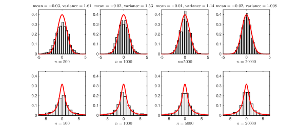
Figure 1: Top: empirical distribution of (6.6) and standard normal density for $p=1000$. Bottom: empirical distribution and theoretical Cauchy distribution of (6.4) for $p=1000$.

References

• [1] A.Β Birnbaum, I.M. Johnstone, B.Β Nadler, and D.Β Paul. Minimax bounds for sparse PCA with noisy high-dimensional data. Ann. Statist., 41(3):1055–1084, 2013.
• [2] F.Β Bunea and L.Β Xiao. On the sample covariance matrix estimator of reduced effective rank population matrices, with applications to fPCA. arXiv:1212.5321v3, December 2012.
• [3] T.T. Cai, Z.Β Ma, and Y.Β Wu. Sparse PCA: Optimal rates and adaptive estimation. Ann. Statist., 41(6):3074–3110, 2013.
• [4] J.Β Dauxois, A.Β Pousse, and Y.Β Romain. Asymptotic theory for the principal component analysis of a vector random function: some applications to statistical inference. J. Multivariate Anal., 12(1):136–154, 1982.
• [5] I.M. Johnstone. On the distribution of the largest eigenvalue in principal components analysis. Ann. Statist., 29(2):295–327, 2001.
• [6] I.M. Johnstone and A.Y. Lu. On consistency and sparsity for principal components analysis in high dimensions. J. Amer. Statist. Assoc., 104(486):682–693, 2009.
• [7] T.Β Kato. Perturbation Theory for Linear Operators. Springer-Verlag, New York, 1980.
• [8] A.Β Kneip and K.J. Utikal. Inference for density families using functional principal component analysis. JASA, 96(454):519–532, 2001.
• [9] V.Β Koltchinskii. Asymptotics of spectral projections of some random matrices approximating integral operators. In High dimensional probability (Oberwolfach, 1996), volumeΒ 43 of Progress in Probability, pages 191–227. BirkhΓ€user, Basel, 1998.
• [10] V.Β Koltchinskii and K.Β Lounici. Asymtotics and concentration bounds for bilinear forms of spectral projectors of sample covariance, 2014. Arxiv:1408.4643.
• [11] V.Β Koltchinskii and K.Β Lounici. Concentration inequalities and moment bounds for sample covariance operators. In Bernoulli, to appear. ArXiv:1405.2468.
• [12] K.Β Lounici. Sparse principal component analysis with missing observations. High dimensional probability VI, Progress in Probability, Institute of Mathematical Statistics (IMS) Collections, 66:327–356, 2013.
• [13] D.Β Paul. Asymptotics of sample eigenstructure for a large dimensional spiked covariance model. Statist. Sinica, 17(4):1617–1642, 2007.
• [14] R.Β Vershynin. Introduction to the non-asymptotic analysis of random matrices. In Compressed sensing, pages 210–268. Cambridge Univ. Press, Cambridge, 2012.
• [15] V.Β Vu and J.Β Lei. Minimax rates of estimation for sparse PCA in high dimensionspca in high dimensions. JMLR, 22:1278–1286, 2012.