Vlasov versus $N$-body: the Hénon sphere

Abstract

We perform a detailed comparison of the phase-space density traced by the particle distribution in Gadget simulations to the result obtained with a spherical Vlasov solver using the splitting algorithm. The systems considered are apodized Hénon spheres with two values of the virial ratio, $R\simeq 0.1$ and $0.5$. After checking that spherical symmetry is well preserved by the $N$-body simulations, visual and quantitative comparisons are performed. In particular we introduce new statistics, correlators and entropic estimators, based on the likelihood of whether $N$-body simulations actually trace randomly the Vlasov phase-space density. When taking into account the limits of both the $N$-body and the Vlasov codes, namely collective effects due to the particle shot noise in the first case and diffusion and possible nonlinear instabilities due to finite resolution of the phase-space grid in the second case, we find a spectacular agreement between both methods, even in regions of phase-space where nontrivial physical instabilities develop. However, in the colder case, $R=0.1$, it was not possible to prove actual numerical convergence of the $N$-body results after a number of dynamical times, even with $N=10^{8}$ particles.

1 Introduction

Stars in galaxies and dark matter in the Universe can be modeled in phase-space as self-gravitating collisionless fluids obeying the Vlasov-Poisson equations:

$$\frac{\partial f}{\partial t}+\mn@boldsymbol{u}.\nabla_{\mn@boldsymbol{r}}f-\nabla_{\mn@boldsymbol{r}}\phi.\nabla_{\mn@boldsymbol{u}}f=0,$$ (1)

$$\Delta_{\mn@boldsymbol{r}}\phi=4\pi G\rho=4\pi G\int f(\mn@boldsymbol{r},\mn@boldsymbol{u},t)\ {\rm d}\mn@boldsymbol{u},$$ (2)

where $f(\mn@boldsymbol{r},\mn@boldsymbol{u},t)$ represents the phase-space density at position $\mn@boldsymbol{r}$ and velocity $\mn@boldsymbol{u}$, $\phi$ is the gravitational potential, and $G$ is the gravitational constant.

In general, these equations do not have simple analytical solutions. They are therefore often solved numerically. The most widely used numerical scheme is the $N$-body approach and there exist many different implementations, which mainly differ from each other in the way Poisson equation is solved (see, e.g., Bertschinger, 1998; Colombi, 2001; Dolag et al., 2008; Dehnen & Read, 2011, for reviews on the subject). The $N$-body method attempts to sample the phase-space density by an ensemble of Dirac functions that represent particles interacting with each other through gravitational force. In order to avoid numerical artefacts due to the $1/r^{2}$ divergence of the force at small distances, the gravitational potential is usually replaced by an effective one so that the force is smoothed at scales smaller than a softening parameter $\epsilon$. This procedure corresponds to assuming that the particles are clouds of size ${\cal\epsilon}$ interacting with each other.

Approximating the phase-space density with macro-particles, however, has its own limitation. In particular, the close $N$-body encounter is one of the most notable sources of numerical artefacts, in addition to more subtle collective effects induced by the discrete nature of the distribution of the particles (see, e.g. Aarseth, Lin, & Papaloizou, 1988; Splinter et al., 1998; Boily, Athanassoula, & Kroupa, 2002; Binney, 2004; Joyce, Marcos, & Sylos Labini, 2009). Of course, the time integration scheme and the way to solve the Poisson equation numerically are well-known sources of errors, even though not particular to the $N$-body method.

There are several previous studies that discussed the limitations of the $N$-body results, including underestimating strong numerical artefacts, particularly in the cold case where the initial velocity dispersion is null (see, e.g., Melott et al., 1997; Melott, 2007), and long-term nonlinear resonant modes induced by the discrete nature of the particles (see, e.g., Alard & Colombi, 2005; Colombi & Touma, 2014). We also note that it is not yet obvious that the fine inner structure of dark matter halos is completely understood from physical and even numerical points of view, despite numerous intensive convergences studies of the $N$-body approach (see, e.g., Moore et al., 1998; Jing & Suto, 2000, 2002; Power et al., 2003; Springel et al., 2008; Stadel et al., 2009).

It is therefore highly desired to develop alternative numerical methods to the traditional $N$-body approach so that one can understand better its validity and fundamental limitations.

In the cold case, relevant to the current paradigm of cold dark matter scenario, the phase-space distribution function is supported by a three-dimensional sheet evolving in six-dimensional phase-space, which can be partitioned in a continuous way with an ensemble of tetrahedra as proposed in recent works (see, e.g., Shandarin, Habib, & Heitmann, 2012; Hahn, Abel, & Kaehler, 2013). Unfortunately, the increasing complexity of the structure of the system during evolution requires more and more sampling elements, and the computational cost becomes prohibitive after several dynamical time-scales.

In this article, we consider the warm case, in which the system presents a non-negligible initial local velocity dispersion component relative to gravitational potential energy. In this case, the phase-space distribution function has to be sampled on a 6-dimensional mesh, which makes again the computational cost very high. Therefore, we shall restrict to spherical systems, hence reducing the actual number of dimensions of the dynamical setup to three.

There exist many methods to solve the Vlasov-Poisson equations in the warm case, mainly developed in plasma physics. One of the most famous solvers is the splitting algorithm of Cheng & Knorr (1976) and its numerous extensions (see, e.g. Shoucri & Gagne, 1978; Sonnendrücker et al., 1999; Filbet, Sonnendrücker, & Bertrand, 2001; Besse & Sonnendrücker, 2003; Alard & Colombi, 2005; Umeda, 2008; Besse et al., 2008; Crouseilles, Mehrenberger, & Sonnendrücker, 2010; Campos Pinto, 2011; Rossmanith & Seal, 2011; Güçlü, Christlieb, & Hitchon, 2014, but this list is far from complete). This algorithm, that we shall adopt below, exploits directly the Liouville theorem: the phase-space density $f(\mn@boldsymbol{r},\mn@boldsymbol{v},t)$ is conserved along motion. Then the equations of the dynamics during each time step are divided into “drift” and “kick” parts according to Hamiltonian dynamics and are solved backwards:

$$f^{*}(\mn@boldsymbol{r},\mn@boldsymbol{u}) = f(\mn@boldsymbol{r}-\mn@boldsymbol{u}\Delta t/2,\mn@boldsymbol{u},t),\quad{\rm Drift},$$ (3)

$$f^{**}(\mn@boldsymbol{r},\mn@boldsymbol{u}) = f^{*}(\mn@boldsymbol{r},\mn@boldsymbol{u}+\nabla_{\mn@boldsymbol{r}}\phi\Delta t),\quad{\rm Kick},$$ (4)

$$f(\mn@boldsymbol{r},\mn@boldsymbol{u},t+\Delta t) = f^{**}(\mn@boldsymbol{r}-\mn@boldsymbol{u}\Delta t/2,\mn@boldsymbol{u}),\quad{\rm Drift},$$ (5)

where $\nabla_{\mn@boldsymbol{r}}\phi$ is computed from $f^{*}$. In practice the phase-space distribution function is sampled on a mesh, and each step is performed by using tracer particles located at mesh sites and following the equations of motion split as above. Resampling of $f^{*}$, $f^{**}$ and finally the phase-space distribution function at the next time step is performed by using an interpolation, e.g. based on the spline method.

The splitting scheme was applied for the first time in astronomy in early 1980’s, to one dimensional systems (Fujiwara, 1981), galactic disks (Watanabe et al., 1981; Nishida et al., 1981) and spherical systems (Fujiwara, 1983). Nevertheless, it has been almost forgotten since then except for a few contributions (e.g., Hozumi, Fujiwara, & Kan-Ya, 1996; Hozumi, Burkert, & Fujiwara, 2000) that include a recent preliminary investigation of the algorithm in full 6-dimensional phase-space (Yoshikawa, Yoshida, & Umemura, 2013).

As mentioned above, however, solving fully six-dimensional phase-space problems with sufficient accuracy is still very unrealistic now. In this article, therefore, we focus on spherical systems, where phase-space is only three dimensional: the three coordinates of interest are the radial position $r$, the radial velocity $v$ and the angular momentum $j$. Following earlier works performed in the framework of one dimensional gravity (see, e.g., Mineau, Feix, & Rouet, 1990), we carry out a detailed comparison between an $N$-body code, Gadget (Springel, Yoshida, & White, 2001; Springel, 2005), and an improved version of the splitting algorithm implementation by Fujiwara (1983), VlaSolve.

Our goal is to check how well the particle distribution in Gadget traces the phase-space density obtained from VlaSolve, and to see how the results depend on various parameters of the simulations, in particular the number of particles in the $N$-body simulations and the spatial resolution in the Vlasov code. We would however like to emphasize here that the purpose of this article is not to compare the performance of the two codes from the view-point of computational cost.

While a fairly good physical insight is obtained through visual inspection of the resulting phase-space density plots, we also present a more quantitative comparison. To do so, we introduce correlators and entropic estimators based on a likelihood approach, ans ask whether the $N$-body simulations can be considered as local Poisson realizations of the Vlasov code phase-space density.

Because of our restrictive choice of the geometry of the system, it is important to simulate spherical configurations that are known to be stable against small anisotropic perturbations induced by the shot noise of the particles. Indeed, we shall use the public treecode Gadget without any specific modification to enforce spherical dynamics. Although an alternative approach consisting in enforcing pure radial dynamics in Gadget (see, e.g., Huss, Jain, & Steinmetz, 1999) may facilitate comparisons with the Vlasov code, we do not adopt this approach in order to avoid any possible subtle biases in the analyses.

In this respect, the Hénon sphere (Hénon, 1964) is particularly suited for our purpose since it is known to preserve well its spherical nature during the course of dynamics even when being simulated with a $N$-body technique and, in particular, it is not prone to radial orbit instability (see, e.g., van Albada, 1982; Hozumi, Fujiwara, & Kan-Ya, 1996; Roy & Perez, 2004; Barnes, Lanzel, & Williams, 2009). In this configuration, the initial phase-space distribution function is isotropic and Gaussian distributed in velocity space and given by

$$f_{\rm H}(r,v,j) = \frac{\rho_{0}}{(2\pi\sigma_{v}^{2})^{3/2}}\exp\left(-\frac{1}{2}\frac{v^{2}+j^{2}/r^{2}}{\sigma_{v}^{2}}\right),$$ (6)

$$\quad\quad\quad\quad\quad\quad\quad\quad\quad\quad\quad\quad\quad r\leq R_{\rm H},$$

with $(4\pi/3)\rho_{0}R_{\rm H}^{3}=M$, the total mass of the system. In the simulations discussed in this article, we work in units where $G=1$, and the initial radius of the Hénon sphere and its total mass are chosen to be

$$M=1,\quad R_{\rm H}=2,$$ (7)

which fixes $\sigma_{v}$ in equation (6) once the virial ratio is given.

We shall consider “warm” and “cold” settings, which correspond to the initial virial ratio $R=|2T/W|=5R_{\rm H}\sigma_{v}^{2}/M$ of $\approx 0.5$ and $\approx 0.1$, respectively, where $T$ and $W$ are the total kinetic and potential energy of the system. The two classes of initial conditions exhibit distinct features, in particular concerning the metastable state to which the system relaxes through phase mixing. The warm system builds a core-halo structure, with the halo displaying a power-law profile $\rho(r)\sim r^{-4}$ (see, e.g., Hénon, 1964; Gott, 1973; van Albada, 1982). In contrast, the cold system develops a more concentrated smaller core (see, e.g., van Albada, 1982; Sylos Labini, 2012), but never reaches a strictly stationary regime because a significant fraction of the mass acquires positive energy and escapes from the system (see, e.g., van Albada, 1982; Joyce, Marcos, & Sylos Labini, 2009; Sylos Labini, 2012).

This article is organized as follows. In § 2 we describe our Vlasov solver, VlaSolve. Section 3 provides information about the $N$-body runs and the parameters used in Gadget. In § 4, we check that the $N$-body simulations stay indeed spherical during evolution. Section 5 presents a visual inspection of the phase-space density, which is followed by a quantitative statistical analysis in § 6. Finally, § 7 summarizes and discusses our present results.

2 The Vlasov code: VlaSolve

Under spherical symmetry, the Vlasov equation reads

$$\frac{\partial f}{\partial t}+v\frac{\partial f}{\partial r}+\left(\frac{j^{2}}{r^{3}}-\frac{GM_{r}}{r^{2}}\right)\frac{\partial f}{\partial v}=0,$$ (8)

where $v$ is the radial component of the velocity, $j$ is the angular momentum, $M_{r}=M\left(<r\right)$ is the mass inside a sphere of radius $r$.

Our code VlaSolve solves equation (8) numerically with the splitting algorithm, following closely Fujiwara (1983).

Phase space is discretized into a rectangular mesh of size $(N_{r},N_{v},N_{j})$ for $R_{\rm min}\leq r\leq R_{\rm max}$, $-v_{\rm max}\leq v\leq v_{\rm max}$, and $0\leq j\leq J_{\rm max}$. More specifically, we use a logarithmically equal interval for $r$, a linearly equal interval for $v$. The $k^{\rm th}$-bin of the angular momentum slice corresponds to the interval $[J_{\rm max}(k-1)^{2}/N_{j}^{2},J_{\rm max}k^{2}/N_{j}^{2}]$ and is represented by $j_{k}=J_{\rm max}(k-1/2)^{2}/N_{j}^{2}$.

We modify the splitting algorithm using the fact that the angular momentum is an invariant of the Hamiltonian system. Hence, one may treat each slice with a different value of $j$ in phase-space independently, except for gravitational coupling via the Poisson equation. We include the inertial component of the force, $j^{2}/r^{3}$, in the “drift” step (equations 3 and 5), while the “kick” step (equation 4) corresponds solely to gravitational force:

$$f^{*}(r,v,j) = f[r^{*}(-\Delta t/2),v^{*}(-\Delta t/2),j,t],$$ (9)

$$f^{**}(r,v,j) = f^{*}(r,v+GM_{r}/r^{2}\Delta t,j),$$ (10)

$$f(r,v,j,t+\Delta t) = f^{**}[r^{*}(-\Delta t/2),v^{*}(-\Delta t/2),j],$$ (11)

where $r^{*}$ and $v^{*}$ solve analytically the motion in absence of gravity starting from coordinates $(r,v,j)$ in phase-space (see, e.g., Colombi & Touma, 2008):

$${r}^{*}(h) = \sqrt{\frac{\left[\sqrt{2r^{2}H_{\rm K}-j^{2}}+2\ {\rm sgn}(v)H_{\rm K}h\right]^{2}+j^{2}}{2H_{\rm K}}},$$ (12)

$${v}^{*}(h) = {\rm sgn}(v)\sqrt{2H_{\rm K}-\frac{j^{2}}{{r^{*}(h)}^{2}}},$$ (13)

with $H_{\rm K}\equiv v^{2}/2+j^{2}/(2r^{2})$ (when $v^{*}<0$, these equations are valid until $v^{*}=0$).

Because a non-zero angular momentum bends the trajectories in $(r,v)$ space, the drift step requires a two-dimensional interpolation of the phase-space distribution function in $(r,v)$ space, while the kick step, which only modifies the velocities, can be completed with a one-dimensional interpolation. We follow Fujiwara (1983), and carry out the interpolations using third-order splines. In this interpolation scheme, however, the positivity of the phase-space distribution function is not warranted, and numerical aliasing and diffusion effects are expected when the phase-space distribution function varies over scales of the order of, or smaller than, the mesh element size.

In order to reduce such numerical artefacts, we modify equation (6) as follows:

$$f_{\rm H}(r,v,j) = \frac{\rho_{0}}{(2\pi\sigma_{v}^{2})^{3/2}}\exp\left(-\frac{1}{2}\frac{v^{2}+j^{2}/r^{2}}{\sigma_{v}^{2}}\right)\times$$ (14)

$$\frac{1}{2}\left[1+{\rm erf}\left(\frac{R_{\rm H}-r}{\Delta}\right)\right],\quad r\leq R_{\rm H},$$

with $\Delta=1/2$. Then we recompute $\rho_{0}$ in equation (6) so that the total mass remains unity. This apodization slightly changes the actual values of the virial ratio to $R\simeq 0.55$ and $0.11$, although we shall still denote them by $0.5$ and $0.1$ just for simplicity. It may also modify the long-term dynamical properties of the original Hénon sphere relative to what is expected. This is why we check again the extent to which the spherical nature of the system is retained in the $N$-body simulations (§ 4).

Adopting a logarithmic binning for $r$ is well suited for tracing small-scale features around the center of the system. This implies, however, that radii smaller than a finite minimum value $R_{\rm min}$ are missing from the computing domain. A conventional trick to overcome the problem is to assume a reflecting boundary at $r=R_{\rm min}$ (see, e.g.. Gott, 1973; Fujiwara, 1983). Usually, a systematic time-lag between orbits in this method is neglected: particles reaching the reflective kernel boundary instantly travel the $2R_{\rm min}$ distance through the central region, while they should actually take a finite time depending on their radial velocity and angular momentum. In VlaSolve, we improve the reflecting sphere method by taking into account the actual time spent by particles travelling inside the region $r\leq R_{\rm min}$, which is made easily possible by neglecting the gravitational force. Technical details about the implementation are provided in Appendix A.1.

To complete algorithmic details, Appendix A.2 discusses the hybrid parallelization of VlaSolve with OpenMP and MPI libraries.

In this paper, we perform 4 simulation runs with different resolutions, each for $R=0.1$ and $0.5$ (Table 1). To cover the dynamical range of interest, the computing mesh uses $R_{\rm min}=0.01$, $R_{\rm max}=25$ and $J_{\rm max}=1.6$. The maximum amplitude of the velocity is $v_{\rm max}=2$ and 4 for $R=0.5$ and $0.1$, respectively. With this choice of the parameters, the computational domains are sufficiently large to contain all the system up to the end of the simulations, which corresponds to $t=100$ for $R=0.5$ and $t=35$ for $R=0.1$. As will be illustrated later in phase-space density plots, these final epochs are sufficient for the system to have relaxed at the coarse level to a meta-stable state through mixing. Strictly speaking, this is not the case in the $R=0.1$ case because a fraction of the mass escapes from the system (see, e.g., van Albada, 1982; Sylos Labini, 2012), as already mentioned in the Introduction.

$N_{r}$ $N_{v}$ $N_{j}$ $\Delta t$ 1024 1024 512 $5\times 10^{-4}$ 512 512 512 $10^{-3}$ 2048 2048 32 $2.5\times 10^{-4}$ 1024 1024 32 $5\times 10^{-4}$

Table 1: The parameters used for the VlaSolve simulations.

We adopt a constant time step $\Delta t$ throughout each simulation. Just to stay on the conservative side, we choose a resolutely small value of $\Delta t$, despite the increased computational cost. Note however that excessively small time step might artificially increase diffusion effects related to successive interpolations of the phase-space distribution function (Hallé, 2015).

In Appendix A.3, a comparison among all the simulations is performed for $R=0.1$. It indicates that diffusion and aliasing effects discussed earlier are indeed significant, despite the apodization of initial conditions, but do not seem to affect the dynamical properties of the system. Note that is tempting to undersample angular momentum space since $j$ is an invariant of the dynamics. However, we show in this appendix that it is not wise to do so, because it can provoke nonlinear instabilities after a few dynamical times.

3 $N$-body simulation with Gadget

We perform the $N$-body simulations using the latest version of the Gadget-2 code (Springel, 2005). Only the treecode part of this “treePM” algorithm is employed. The particle number is varied from $N=10^{4}$ to $10^{7}$ for $R=0.1$ and $0.5$. We also run an additional simulation with $N=10^{8}$ for $R=0.1$.

We choose the parameters for Gadget runs as follows:

• The softening length of the gravitational force is set as $\epsilon=0.2N^{-1/3}$, that is about $1/16$ of the initial mean interparticle distance $(4\pi/3N)^{1/3}R_{\rm H}$ (this estimate neglects the effects of the apodization 14).

• In Gadget, each particle has its individual time step bounded by ${\rm d}t=\min[{\rm d}t_{\rm max},(2\eta\epsilon/|\mn@boldsymbol{a}|)^{1/2}]$, where $\mn@boldsymbol{a}$ is the acceleration of the particle and $\eta$ is a control parameter. We choose $\eta=0.025$ and $\Delta t_{\rm max}=0.01$.

• The tolerance parameter controlling the accuracy of the relative cell-opening criterion (parameter designed by ErrTolForceAcc in the documentation of Gadget, see equation 18 of Springel, 2005) is set as $\alpha_{\rm F}=0.005$.

Appendix B presents the effects of changing these parameters on the phase-space distribution function for simulations with $N=10^{6}$ particles and a virial ratio of $R=0.1$. These analyses, performed at $t=15$, confirm that the parameters used for the simulations of this paper are reasonable. Interestingly, changing the softening length by large factors does not influence much the results, as already noticed previously in the literature (see, e.g. Barnes, Lanzel, & Williams, 2009), as long as it is kept small enough.

4 Consistency check: sphericity of the $N$-body results

Before presenting comparisons between Gadget and VlaSolve, it is necessary to make sure that the sphericity of the system is preserved in the Gadget simulations because our Vlasov runs are performed assuming exact spherical symmetry. Figure 1 shows, for different values of the number of particles $N$, the evolution with time of the ratios $b/a$ and $b/c$, where $a\leq b\leq c$ are the eigenvalues of the inertia tensor of the particle distribution.

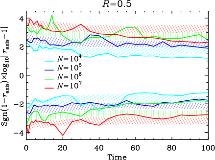
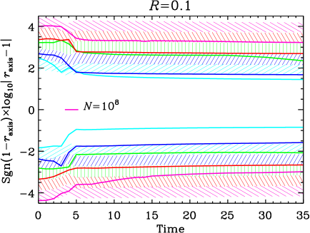
Figure 1: Evolution of the departure from spherical symmetry: ratios of the eigenvalues of the inertia tensor of the system as functions of time in the Gadget simulations. To emphasize the small differences from unity, the quantity ${\rm sgn}(1-r_{\rm axis})\log_{10}|1-r_{\rm axis}|$ is plotted as a function of time, where $r_{\rm axis}=b/a$ (upper curves on each panel) or $b/c$ (lower curves) and $a\leq b\leq c$ are the eigenvalues of the inertia tensor of the Gadget particle distribution. Each color corresponds to a given value of the number $N$ of particles as indicated in the panels. Dashed regions correspond to the one sigma confidence level zone expected for a particle distribution locally Poisson sampling the spherically symmetrical projected density profile $\rho(r,t)$, where $\rho(r,t)$ is estimated from interpolation of the Gadget particle distribution in spherical shells. To calculate the average of $r_{\rm axis}$ and the associated one sigma error contours, 100 local Poisson realizations have been performed for each snapshot and value of $N$ considered, except for $N=10^{7}$ and $N=10^{8}$ (on right panel only for the latter). In the last cases, the dashed regions correspond to an extrapolation of the results obtained from $N=10^{6}$.

The dashed regions correspond to the one sigma zone obtained from an ensemble of 100 local Poisson realizations of the spherical density $\rho(r)$, which is estimated from interpolation over spherical shells from the Gadget particles. From the measurements in Fig. 1, deviations from spherical symmetry due to the particle shot noise can be roughly scaled to

$$\left\langle\frac{b}{a}\right\rangle-1\simeq 1-\left\langle\frac{b}{c}\right\rangle\simeq 2\sigma_{b/a}\simeq 2\sigma_{b/c}\sim\frac{1}{\sqrt{N}},$$ (15)

where $\sigma_{b/a}^{2}$ and $\sigma^{2}_{b/c}$ are the variances of $b/a$ and $b/c$ obtained from the dispersion over the 100 realizations. Note that equation (15) is not intended to be accurate. The asphericity due to discreteness should depend on details of the density profile, as shown in Fig. 1. While it would be possible to compute in a perturbative way the quantities in equation (15) from statistical analysis of the inertia tensor assuming $N\gg 1$ and using error propagation formulae, this is a cumbersome exercise far beyond the scope of this paper.

We also note that another possible source of errors comes from the position of the center of the system. Indeed, an inaccurate determination of the center obviously worsens the apparent agreement with spherical symmetry. In the measurements presented in Fig. 1, the inertia matrix is not computed with respect to the center of gravity of the particle distribution, which can be affected by the fact that some particles can get far away from the system through $N$-body relaxation. Instead, we determine the center of the system using an iterative procedure trying to optimize the match of the phase-space distribution function with that of the Vlasov code, as detailed in § 6.1. This procedure is not free from errors either, and may contribute to the fluctuations observed in the curves of Fig. 1.

Inspection of Fig. 1 shows that the measured ratios $b/a$ and $b/c$ behave differently in the $R=0.5$ and $R=0.1$ simulations. In the $R=0.5$ case, the agreement of the measurements with the Poisson prediction is in general good, with a slight trend to ellipticity, except for the top red curve and the bottom green curve where the deviation from spherical symmetry is larger than the Poisson expectation. Still, in the case of $R=0.5$, the system remains to a very good approximation spherical for all values of $N$, given the expected deviations due to pure statistical noise.

The curves representing the eigenvalue ratios are more steady for $R=0.1$ than for $R=0.5$, which might be slightly puzzling at first sight. However, a very plausible explanation of this difference is that the initial velocity dispersion is larger for $R=0.5$ than for $R=0.1$, hence adding a more prominent random component to the time behavior of the deviation from sphericity.

Regarding $R=0.1$, deviations from spherical symmetry are clearly more significant compared to local Poisson expectations after $t\approx 3$, roughly the collapse time of the sphere. While the $N=10^{4}$ run exhibits a deviation larger than 10 percent, spherical symmetry is confirmed to be a good approximation for $N\geq 10^{5}$.

Finally, we also check deviations from spherical symmetry for subsets of particles in excursions corresponding to $f\geq f_{\rm th}$, where $f$ is the phase-space distribution function measured in the $1024\times 1024\times 512$ VlaSolve runs. For each value of the virial ratio, two thresholds $f_{\rm th}$ are chosen such that the excursions contained initially about 90 and 60 percent of the total mass (see bottom panels of Fig. 6 below). Given the uncertainties in the measurements, the above conclusions still hold: the properties of the deviations from spherical symmetry, that we do not show here for simplicity, do not indeed depend significantly on radius. We only notice a slight improvement in the $R=0.5$ case when considering particles in the excursions.

5 Phase-space density: visual inspection

Now we are ready to perform direct comparisons between the Vlasov and $N$-body simulation results. For this purpose, we consider the phase-space density at different epochs (Figs.  2 to 5 below). To be more specific, we plot the constant angular momentum slice of $f(r,v,j)$ at $j=0.244$, and its integral over the angular momentum:

$$f_{\rm summed}(r,v)=\int f(r,v,j)\ 2\pi j{\rm d}j.$$ (16)

Figures 2 and 3 plot $f(r,v,j\simeq 0.244)$ and $f_{\rm summed}(r,v)$, respectively, for the VlaSolve and Gadget simulations of the warm case, $R=0.5$. In both figures, snapshots at $t=10$, 50, 80 and 100 are plotted from left to right. The panels correspond to the VlaSolve runs with $(N_{r},N_{v},N_{j})=(2048,2048,32)$ and $(1024,1024,512)$, the Gadget runs with $N=10^{7}$, $10^{6}$ and $10^{5}$, from top to bottom.

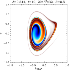
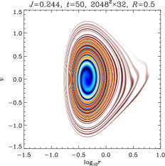
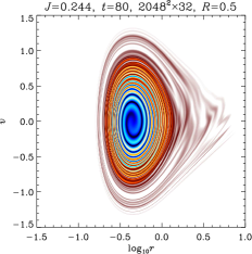
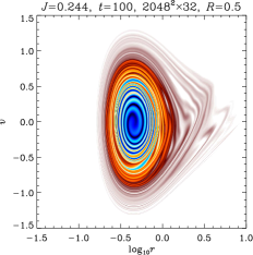
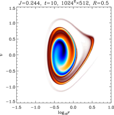
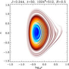
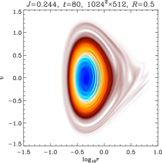
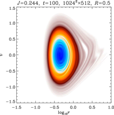
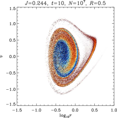
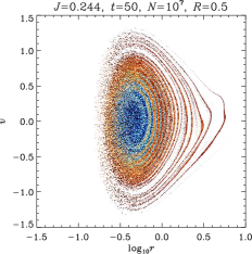
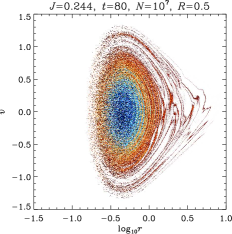
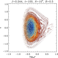
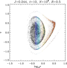
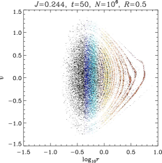
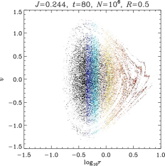
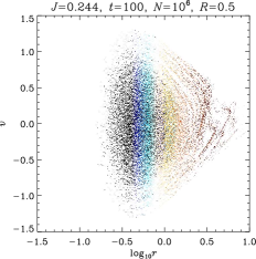
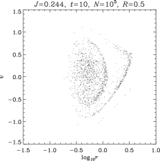
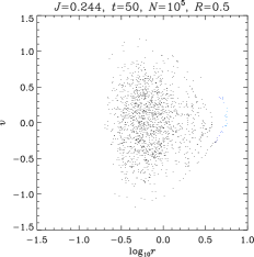
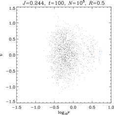
Figure 2: VlaSolve versus Gadget in phase-space: phase-space density for $R=0.5$ and averaged over $j\in I_{J}=[0.225,0.264]$. Each column of panels corresponds to a given value of time $t$, increasing from left to right. The first two lines of panels display $f(r,v,j)$ for VlaSolve simulations with $(N_{r},N_{v},N_{j})=(2048,2048,32)$ and $(1024,1024,512)$ respectively, while the three bottom lines correspond to the $N$-body simulations, with various values of the number of particles $N$ as indicated on each panel. Note that the VlaSolve simulation with $(N_{r},N_{v},N_{j})=(2048,2048,32)$ has only one angular momentum slice, $J=0.244$, in the interval $I_{J}$, so there is no blurring of the filamentary details of $f(r,v,j)$ on the left side of the peak of the distribution function contrarily to the other cases. In the $N$-body case, $f(r,v,j)$ was computed on the same mesh as the $(1024,1024,32)$ VlaSolve simulation using nearest grid point interpolation, which explains the artefacts on the color pattern in the last two lines of panels.

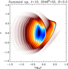
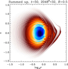
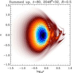
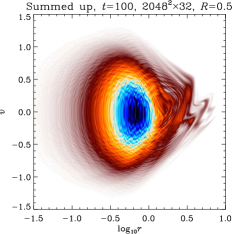
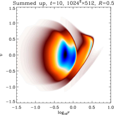
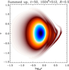
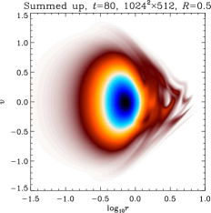
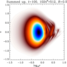
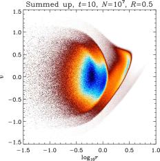
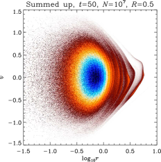
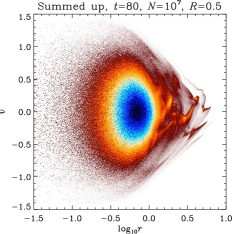
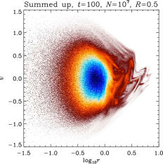
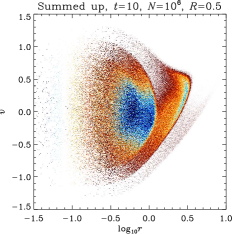
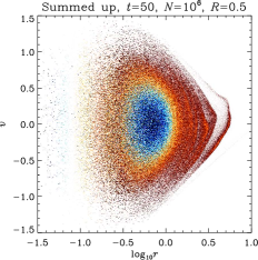
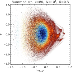
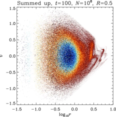
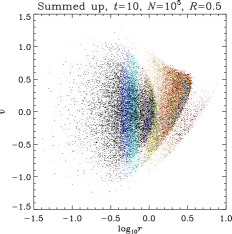
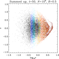
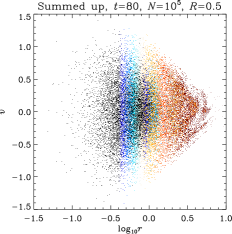
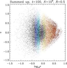
Figure 3: Same as in Fig. 2, but the phase-space distribution function has now been summed up over the whole available range of values of $j\in[0,J_{\rm max}=1.6]$, where $J_{\rm max}$ is the maximum sampled value of $j$ for the VlaSolve simulations.

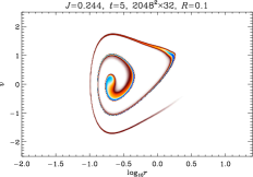
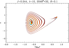
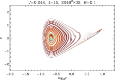
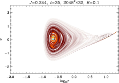
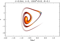
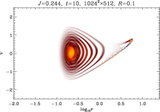
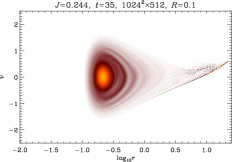
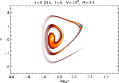
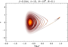
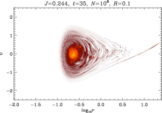
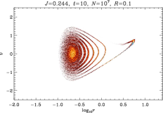
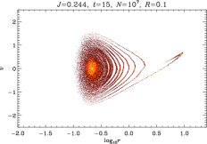
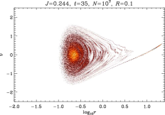
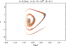
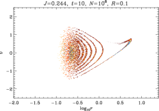
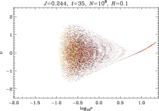
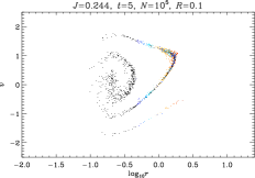
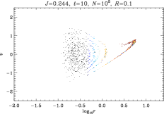
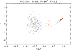
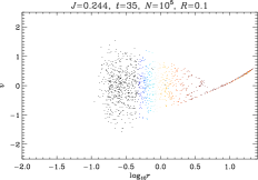
Figure 4: Same as in Fig. 2, but for a colder initial configuration with virial ratio $R=0.1$. There is also an additional line of panels corresponding to the Gadget simulation with $N=10^{8}$ particles. Note the large $R$ tail escaping from the system, corresponding to a fraction of the mass with positive energy (see, e.g., van Albada, 1982; Joyce, Marcos, & Sylos Labini, 2009; Sylos Labini, 2012).

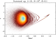
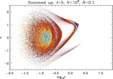
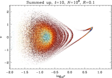
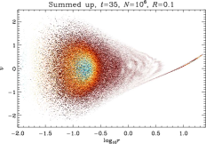
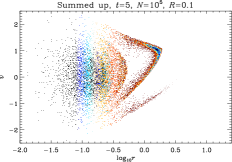
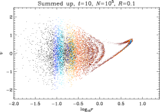
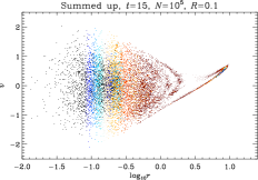
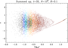
Figure 5: Same as in Fig. 3, but for $R=0.1$ and with the additional $N$-body simulation involving $N=10^{8}$ particles.

The overall conclusion of the visual inspection of Figs. 2 and 3 is that the Vlasov solver and the $N$-body code exhibit very good agreement with each other, probably even much more than expected. In particular, both results present a remarkably similar instability in the region $1\mathrel{\mathchoice{\vbox{\offinterlineskip\halign{\hfil$\displaystyle#$\hfil\cr<\cr\sim\cr}}}{\vbox{\offinterlineskip\halign{\hfil$\textstyle#$\hfil\cr<\cr\sim\cr}}}{\vbox{\offinterlineskip\halign{\hfil$\scriptstyle#$\hfil\cr<\cr\sim\cr}}}{\vbox{\offinterlineskip\halign{\hfil$\scriptscriptstyle#$\hfil\cr<\cr\sim\cr}}}}r\mathrel{\mathchoice{\vbox{\offinterlineskip\halign{\hfil$\displaystyle#$\hfil\cr<\cr\sim\cr}}}{\vbox{\offinterlineskip\halign{\hfil$\textstyle#$\hfil\cr<\cr\sim\cr}}}{\vbox{\offinterlineskip\halign{\hfil$\scriptstyle#$\hfil\cr<\cr\sim\cr}}}{\vbox{\offinterlineskip\halign{\hfil$\scriptscriptstyle#$\hfil\cr<\cr\sim\cr}}}}10^{0.8}$, even in details, showing a surprising reliability of the conventional $N$-body approach for these particular initial conditions.

However, before reaching this conclusion, one has to take into account several limiting factors. In particular, we should bear in mind the fact that the VlaSolve simulations are subject to significant diffusion, which smears out fine details of the phase-space distribution function. This diffusion effect is clearly visible at $t=50$, when comparing the outer filamentary structures observed in the Vlasov simulations to the $N$-body result. Putting aside this coarse-graining effect, the structures are exactly similar in both the $N$-body and Vlasov simulations at $t\leq 50$, even including small gaps in the phase-space distribution function related to nonlinear instabilities that start building up. These instabilities grow further at later epochs. They are considerably smeared out in the $(1024,1024,512)$ VlaSolve simulation but unquestionably present. Adding resolution in $(r,v)$ space (at the cost of resolution in $j$) improves the agreement with Gadget, which confirms that the instabilities observed in the Gadget simulations are physical and not of numerical nature.

Figure 2 indicates that lowering the number of particles in the $N$-body simulations may be interpreted as a coarse-graining: it makes finer details more fuzzy but still keeps global features of the phase-space density correctly. We also note that using a small number of slices in $j$ in the Vlasov solver does not seem to alter the dynamical properties of the system despite the considerable level of aliasing it introduces.

The situation is more complicated for the cold case, $R=0.1$ (Figs. 4 and 5). Up to $t\simeq 10$, the above conclusions for $R=0.5$ are still valid. However, some instabilities emerge at $t\simeq 10$ in the Gadget simulations with $N\leq 10^{6}$ particles as well as the $(2048,2048,32)$ Vlasov run. Until this epoch, the $N\geq 10^{7}$ and the $(1024,1024,512)$ simulations agree perfectly with each other (modulo the smearing effects already discussed above) and present a smooth phase-space density without any sign of instability. On the other hand, the other simulations exhibit slightly irregular phase-space density. Such a trend is easily seen in Fig. 4, even though not so obvious in the $(2048,2048,32)$ Vlasov simulation. These irregularities appear as well in the $N\geq 10^{7}$ simulations but at later epochs, and then develop in a dramatic way. A careful inspection of successive snapshots of the simulations indeed suggests that the onset of these irregular patterns comes later with increasing $N$.

As discussed in Appendices B and A.3, these instabilities result from the discrete nature of the system in the $N$-body case, and from the aliasing effect due to sparse-sampling of the angular momentum space in the Vlasov code. Since the pattern of the instabilities changes significantly from one simulation to another unlike the $R=0.5$ case, they should be due to numerical, not physical, origin.

As shown in Appendix B, their presence is very insensitive to the choice of softening, time step or parameters controlling force accuracy in Gadget. They can therefore be reduced only by increasing the number of particles and the resolution in the Gadget and VlaSolve simulations, respectively.

It is important to notice that even the $N=10^{8}$ result might be insufficient to describe properly the system at late epochs. In the $(1024,1024,512)$ Vlasov simulation, the phase-space distribution function seems to be rather smooth at all times and the system is free of instability, contrarily to the $R=0.5$ case. However, it is difficult at this point to know if actual physical instabilities build up at late times in the $R=0.1$ case, because diffusion in the Vlasov simulation might prevent the appearance of some unstable modes.

While the irregular patterns observed in Figs. 4 and 5 are definitely of numerical nature, the fact that they develop so easily may indicate that the system is prone to react nonlinearly to small perturbations. Uneven gaps between the filaments of the phase-space density can be observed at $t=15$ (third column of Fig. 4), even in the $(1024,1024,512)$ Vlasov simulation, and one might expect that they correspond to seeds of actual physical instabilities. In this respect, the system might actually develop, at some point, physical unstable modes. These results are quite suggestive of what was obtained previously with a spherical shell code for cold and self-similar systems (Henriksen & Widrow, 1997).

Even with our $N=10^{8}$ particle simulation, it is not clear whether these unstable modes dominate over collective effects due to discreteness. A better understanding of the phenomenon would require a convergence study using even higher-resolution simulations.

6 Statistical analysis

6.1 Correlators and entropic estimators: definitions and concepts

To perform a more accurate analysis, one can try to quantify to which extent the particle distribution in the $N$-body simulations can be considered as a local Poisson process of the phase-space density calculated in the semi-Lagrangian code. To do so, we use, in addition to entropic measurements described further, the following correlators,

$$C_{k}\equiv\frac{\mu_{k}}{\kappa_{k}},$$ (17)

with

$$\mu_{k} = \frac{M}{N}\sum_{i=1}^{N}[f(\Omega_{i})]^{k},$$ (18)

$$\kappa_{k} = \int[f(\Omega)]^{k+1}{\rm d}\Omega.$$ (19)

In these equations, $k$ is a positive integer, $f$ the VlaSolve phase-space density, $M$ the total mass, ${\rm d}\Omega\equiv 2\pi{\rm d}r\times{\rm d}v\times j{\rm d}j$ and $\Omega_{i}=(r_{i},v_{i},j_{i})$, where $r_{i}$, $v_{i}$ and $j_{i}$ are respectively the radial position, radial velocity and angular momentum of each particle of the Gadget simulation.

For a point set randomly sampling a smooth density distribution $g$, the probability density $p(\Omega)$ of having a given particle at phase-space position $\Omega$ is independent from the rest of the particle distribution and is simply proportional to $g(\Omega)$:

$$p(\Omega){\rm d}\Omega=\frac{g(\Omega)}{M}{\rm d}\Omega.$$ (20)

The density probability of having $N$ particles at respective positions $\Omega_{1}$, $\Omega_{2}$, $\ldots$, $\Omega_{N}$ is given by

$${\cal P}(\Omega_{1},\cdots,\Omega_{N})=\prod_{i=1}^{N}p(\Omega_{i}).$$ (21)

Ensemble averaging of $\mu_{k}$ under the law $g$ then reads

$$\langle\mu_{k}\rangle_{g} = \frac{M}{N}\int\sum_{i=1}^{N}[f(\Omega_{i})]^{k}\ {\cal P}(\Omega_{1},\cdots,\Omega_{N})\ {\rm d}\Omega_{1}\cdots{\rm d}\Omega_{N},$$ (23)

$$= \frac{M}{N}\sum_{i=1}^{N}\int_{\Omega}\frac{1}{M}[f(\Omega_{i})]^{k}g(\Omega_{i}){\rm d}\Omega_{i},$$

$$\quad\quad\quad\quad\times\prod_{j\neq i}\int_{\Omega_{j}}\frac{g(\Omega_{j})}{M}{\rm d}\Omega_{j}$$

$$= \int[f(\Omega)]^{k}g(\Omega){\rm d}\Omega,$$ (24)

and

$$\langle C_{k}\rangle_{g}=\frac{\int[f(\Omega)]^{k}g(\Omega){\rm d}\Omega}{\int[f(\Omega)]^{k+1}{\rm d}\Omega}.$$ (25)

Hence, if the distributions $g$ and $f$ coincide, i.e., in our case, if Gadget actually Poisson samples the VlaSolve phase-space density, one obtains $\langle C_{k}\rangle_{g=f}=1$ after ensemble averaging.

When increasing $k$, more weight is given to regions in phase-space corresponding to larger values of $f$. For a point process totally anticorrelated with $f$, $C_{k}$ cancels, while its largest possible value is given by $C_{k}=(M\max f^{k})/\kappa_{k}>1$, when all the particles stay in the region where $f$ is maximal.

An important issue is to compute properly the center of the system position in the Gadget simulations. In order to do this, we find the coordinate origin maximizing $C_{1}$, even though the result of such a procedure can potentially lead to $C_{1}>1$, to optimize the match between concentrations of particles and local extrema of $f$.

The variance of $C_{k}$ can also be calculated in an analogous way to $\langle\mu_{k}\rangle_{g}$:

$$\Delta C_{k}^{2} \equiv \langle C_{k}^{2}\rangle_{g}-\langle C_{k}\rangle^{2}_{g}$$ (26)

$$= \frac{1}{\kappa_{k}^{2}}\left[\frac{M}{N}\langle\mu_{2k}\rangle_{g}-\frac{1}{N}\langle\mu_{k}\rangle^{2}_{g}\right],$$ (27)

which reduces to $\Delta C_{k}^{2}=(M/N)(\kappa_{2k}/\kappa_{k}^{2})-1/N$ when $f$ and $g$ coincide. In practice, we shall use the following estimator for this statistical error:

$$\Delta C_{k}^{2}\simeq\frac{1}{\kappa_{k}^{2}}\left[\frac{M}{N}\mu_{2k}-\frac{1}{N}\mu_{k}^{2}\right],$$ (28)

where $\mu_{2k}$ and $\mu_{k}$ are directly estimated from the $N$-body simulation.

The log-likelihood that the Gadget particle distribution locally Poisson samples the VlaSolve phase-space density $f$ can be written, following the reasoning that leads to equation (21),

$$\ln{\cal L}=\sum_{i=1}^{N}\ln\left[\frac{f(\Omega_{i})}{M}\right].$$ (29)

However, the region ${\cal D}$ where $f>0$ being of finite extent, one expects $\ln{\cal L}=-\infty$ as soon as a particle escapes ${\cal D}$, which is very likely, due for instance to $N$-body relaxation. Furthermore, the Vlasov solver does not guaranty the positivity of $f$. To take into account in a fair way both the defects of the $N$-body and the Vlasov simulations, it is better to restrict to a region ${\cal D}_{\rm th}$ where $f$ is strictly positive:

$$D_{\rm th}\equiv\{\Omega\ {\rm such}\ {\rm that}\ f(\Omega)\geq f_{\rm th},\ f_{\rm th}>0\}.$$ (30)

The log-likelihood of having $Q\leq N$ particles in the region ${\cal D}_{\rm th}$ and the rest outside it (leaving the freedom of the remaining particles to span all the space outside ${\cal D}_{\rm th}$) is given by a binomial law:

$$\ln{\cal L}_{\rm b}(Q,\nu)=\ln\left[\frac{N!}{(N-Q)!Q!}\nu^{Q}(1-\nu)^{N-Q}\right],$$ (31)

where $\nu$ is the fractional mass inside ${\cal D}_{\rm th}$ in the VlaSolve simulation. Hence, equation (29) simply becomes

$$\ln{\cal L}=\sum_{\Omega_{i}\in{\cal D}_{\rm th}}\ln\left[\frac{f(\Omega_{i})}{M_{\rm th}}\right]+\ln{\cal L}_{\rm b}(Q_{\rm th},\nu),$$ (32)

where $Q_{\rm th}$ is the number of particles of the ${\tt Gadget}$ simulation inside ${\cal D}_{\rm th}$ and $M_{\rm th}=\int_{D_{\rm th}}{\rm d}\Omega\ f(\Omega)$.

Note that the distribution of particles which maximizes the first term in equation (32) corresponds again to the case where all the particles of ${\cal D}_{\rm th}$ stay in the region where $f$ is maximal, similarly to the case when the correlator $C_{k}$ is equal to its maximum possible value. Clearly, this situation is not typical, but it is in fact the most likely to consider when it can take place: this is why we maximize $C_{1}$ to estimate the center of the $N$-body system, even though it might turn to be larger than unity.

The expectation value of $\ln{\cal L}$ under the law $f$ can be obtained by ensemble averaging:

$$S(f_{\rm th}) \equiv -\frac{1}{\nu N}\langle\ln{\cal L}\rangle_{f}=S_{f}(f_{\rm th})+S_{\rm b}(f_{\rm th}),$$ (33)

$$S_{f}(f_{\rm th}) \equiv -\int_{D_{\rm th}}\frac{f(\Omega)}{M_{\rm th}}\ln\left[\frac{f(\Omega)}{M_{\rm th}}\right]{\rm d}\Omega,$$ (34)

$$S_{\rm b}(f_{\rm th}) \equiv -\frac{1}{\nu N}\sum_{Q=0}^{N}{\cal L}_{\rm b}(Q,\nu)\ln{\cal L}_{\rm b}(Q,\nu).$$ (35)

In the limit $f_{\rm th}\rightarrow 0$, the quantity $S_{f}(f_{\rm th})$ reduces to the Gibbs entropy of the system, which explains the choice of notations. Moreover, if $N\gg 1$ and if the fractional mass $\nu$ inside the domain of interest $D_{\rm th}$ is of order of unity, which is the case for our analyses, the term $S_{\rm b}(f_{\rm th})$ is in practice negligible compared to $S_{f}(f_{\rm th})$, so $S(f_{\rm th})$ depends only weakly on the total number of particles, as expected.

The variance of $\ln{\cal L}$ can be calculated likewise

$$\sigma_{L}^{2} \equiv \frac{1}{(\nu N)^{2}}\left[\langle\ln{\cal L}^{2}\rangle_{f}-\langle\ln{\cal L}\rangle_{f}^{2}\right]$$

$$\simeq \frac{1}{\nu N}\left\{\int_{D_{\rm th}}\frac{f(\Omega)}{M_{\rm th}}\ln^{2}\left[\frac{f(\Omega)}{M_{\rm th}}\right]{\rm d}\Omega-\nu[S(f_{\rm th})]^{2}\right\},$$

where we have neglected, following the arguments developed earlier, the contributions of $S_{\rm b}$ to the error.

To understand better the interest of using the statistics given by equation (32), one can introduce the difference between the measured value of the log-likelihood and its expectation under the law $f$:

$$\delta S=\frac{1}{\nu N}\left[\langle\ln{\cal L}\rangle_{f}-\ln{\cal L}\right],$$ (38)

where ${\cal L}$ is given by expression (32) calculated for $\Omega_{i}$ extracted from a Gadget simulation. The quantity $\delta S$ estimates the magnitude of the difference between the underlying smooth phase-space density $g$ sampled by Gadget and the VlaSolve phase space density, $f$: its ensemble average other many Gadget realizations indeed reads, when neglecting the binomial term in equation (32),

$$\langle\delta S\rangle_{g}\simeq\int_{f\geq f_{\rm th}}\frac{1}{M_{\rm th}}[g(\Omega)-f(\Omega)]\ln\left[\frac{f(\Omega)}{M_{\rm th}}\right]{\rm d}\Omega.$$ (39)

Under the assumption that the $N$-body simulation Poisson samples the distribution $f$, the magnitude of $\delta S$ should be of the same order of $\sigma_{L}$.

6.2 Correlators and entropic estimators: measurements

Top panels of Fig. 6 show the quantity $S_{f}(f_{\rm th})$ as a function of time for the various VlaSolve simulations we performed and two values of $f_{\rm th}$ chosen such that approximately 90 percent and 60 percent of the total mass is initially inside the excursion $D_{\rm th}$, respectively. The quantity $S_{f}(f_{\rm th})$ is a Casimir invariant –that is an integral over a function of $f$– and should thus be conserved during runtime if the code was perfect. This not the case because of diffusion and aliasing effects in $(r,v)$ space: deviation from conservation of $S_{f}$ happens shortly after collapse time. Then there is a strong mixing phase during which $S_{f}$ increases, then possibly decreases, according to the value of $f_{\rm th}$, and finally reaches an approximate plateau. Deviation from conservation of $S_{f}$ naturally happens sooner when resolution in $(r,v)$ space is smaller. Resolution in $j$ space does not have much influence on $S_{f}$ because angular momentum is an invariant of the dynamics. However, as clearly shown in § 5 and in Appendix A.3 for $R=0.1$, we already know that sparse sampling in $j$ space is not recommended since it can introduce some instabilities in the dynamics, even though this effect does not affect much our likelihood measurements.

  

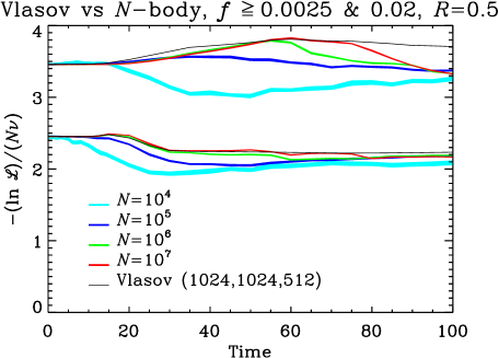
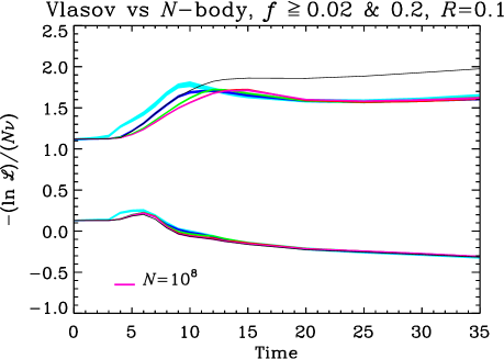
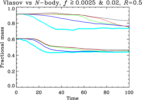
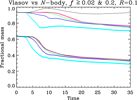
Figure 6: Entropic measurements: effects of VlaSolve resolution (top two panels) and Gadget number of particles (four bottom panels). The left and right panels correspond respectively to $R=0.5$ and $0.1$. On the top panels, the quantity $S_{f}(f_{\rm th})$ given by equation (34) is plotted as a function of time for the Vlasov simulations and for two values of $f_{\rm th}$ indicated on each panel corresponding to approximately initially keeping 90 and 60 percent of the mass inside the excursion. Each curve corresponds to a given resolution as indicated on each panel (the dashes are nearly superposed to the solid line). The top/bottom group of four curves correspond to a smaller/larger value of $f_{\rm th}$. On the middle panels, the solid line is the same as on the top panels, while the colored curves display, for each value of the particle number $N$ in the Gadget simulations, the quantity $-\ln{\cal L}/(N\nu)$ as a function of time, where $\ln{\cal L}$ is given by equation (32). If the $N$-body simulations would Poisson sample the VlaSolve phase-space density, the ensemble average of this quantity over many Gadget realizations should match the solid line (except for a negligible correction due to the $S_{\rm b}$ term in equation 34). Finally, the bottom panels show the fractional mass as a function of time for the two values of $f_{\rm th}$ considered. On the two bottom right panels, there is an additional purple curve nearly indistinguishable from the red one, corresponding to the additional simulation with 100 millions particles we performed for $R=0.1$. In the four bottom panels, the thickness of each colored curve takes into account statistical errors (equation LABEL:eq:errstat for $\ln{\cal L}$). In addition, for the middle panels, systematic errors due to the interpolation of the phase-space distribution function in the VlaSolve simulations also contribute to the estimated errors. In the latter case, we compute $f(\Omega_{i})$ both using nearest grid point and linear interpolation from the values of $f$ on the computational mesh. The difference between the two interpolating methods adds to the thickness of the curves. Note that we use the $(1024,1024,512)$ VlaSolve simulation to perform the comparison to $N$-body results, to minimize the effects of interpolation.

Middle panels of Fig. 6 show the quantity $-\ln{\cal L}/(N\nu)$ measured in Gadget from the particles belonging to the excursion $D_{\rm th}$ as a function of time, where $\ln{\cal L}$ is given by equation (32). For a given value of the threshold $f_{\rm th}$, if the Gadget simulations would actually behave like Poisson realizations of the VlaSolve ones, all the colored curves should be close to the solid line, which corresponds to $S_{f}$. This is clearly not the case for small $f_{\rm th}$ (upper group of curves), except a early times. Increasing the number of particles in the $N$-body simulation improves the agreement with the Vlasov code for $R=0.5$ but does not seem to have a convincing impact in the $R=0.1$ case: for $f_{\rm th}=0.02$, all the $N$-body simulations converge to the same plateau somewhat below the Vlasov code result. On the contrary, for $f_{\rm th}=0.2$ and $R=0.1$, the agreement between Gadget and VlaSolve is striking at all times, except may be for the $N=10^{4}$ simulation during the strong mixing phase. Note also, that at late times, all the $N$-body simulations converge which each other, independently of $f_{\rm th}$ and $R$, except again for the $N=10^{4}$ simulation with $R=0.1$, but we know that this latter presents significant deviations from spherical symmetry and should be probably discarded for the analyses performed here.

To complete the analyses and understand better the results obtained for the log-likelihood, the fractional mass inside the excursions $f\geq f_{\rm th}$ is shown in bottom panels of Fig. 6. Again, this quantity is a Casimir, so it should not change with time in the idealistic case. In practice, while it is difficult to predict the effects of aliasing on the ${\tt VlaSolve}$ mass inside $D_{\rm th}$, diffusion effects are more likely to decrease it, especially by dilution of filamentary structures that build up during the course of dynamics. In the $R=0.5$ case, most of the disagreement between Gadget likelihood and its expectation given by VlaSolve can be understood in terms of fractional mass: effects related to the discrete nature of the $N$-body simulations seem to spread particles away from $D_{\rm th}$. However this process is subtle and seems to remain local as suggested by visual inspection of Figs. 2 and 3. We also checked that it does not affect dramatically the projected density, $\rho(r)$.

In the $R=0.1$ case, the interpretation of the results is slightly more complicated. For $f_{\rm th}=0.2$, the Gadget fractional mass inside the excursion $D_{\rm th}$ behaves similarly as in the $R=0.5$ case as a function of particle number. On the other hand, when examining the quantity $-\ln{\cal L}/(N\nu)$, the $N$-body measurements converge with each other and with VlaSolve much better, especially after relaxation. This means that particles left in $D_{\rm th}$ are redistributed in a non trivial way, such that the effects of the excursion mass loss are compensated. For $f_{\rm th}=0.02$, even the $N=10^{8}$ Gadget sample disagrees with the VlaSolve simulation. Clearly, the Vlasov simulation becomes quickly defective in regions where $f$ is small. On the other hand, convergence of the Gadget simulations at late times might be misleading. Indeed, we noticed from visual inspection of Figs. 4 and 5 that some instabilities appeared in all of them as soon as $t\mathrel{\mathchoice{\vbox{\offinterlineskip\halign{\hfil$\displaystyle#$\hfil\cr>\cr\sim\cr}}}{\vbox{\offinterlineskip\halign{\hfil$\textstyle#$\hfil\cr>\cr\sim\cr}}}{\vbox{\offinterlineskip\halign{\hfil$\scriptstyle#$\hfil\cr>\cr\sim\cr}}}{\vbox{\offinterlineskip\halign{\hfil$\scriptscriptstyle#$\hfil\cr>\cr\sim\cr}}}}15$, although later when $N$ is larger. Interestingly, the measurements in the $N=10^{7}$ and $N=10^{8}$ simulations are nearly indistinguishable from each other, which is a sign that we are nevertheless close to numerical convergence.

Entropic measurements of Fig. 6 are confirmed, at least partly, by Fig. 7.

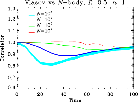
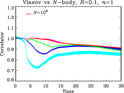
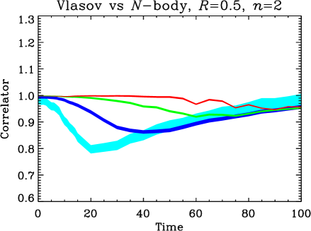
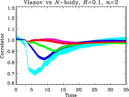
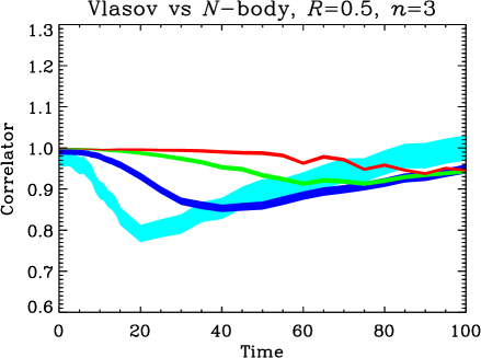
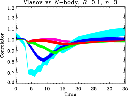
Figure 7: Correlators between VlaSolve and Gadget as functions of time. These quantities, defined in equations (17), (18) and (19), are plotted for $k=1,\ 2,\ 3$ increasing from top to bottom, while left and right panels correspond to $R=0.5$ and $0.1$, respectively. The thickness of the curves, analogously to Fig. 6, takes into account statistical errors according to equation (28) using the measured value of $\nu_{2k}$ and $\nu_{k}$ and systematic errors due to the interpolation of the phase-space density in the VlaSolve samples. Note that there is an additional purple curve on each panel of the right column corresponding to the 100 millions particles simulation.

In particular, a depression of which the depth depends on the number of particles in the $N$-body simulation appears on all the curves. When increasing $N$, the amplitude of the depression decreases and the occurrence of its maximum amplitude is delayed, independently of the actual dynamical state of the system. Again, it can certainly be attributed to collective effects due to Poisson noise. Overall agreement between $N$-body and Vlasov codes improves when increasing the number of particles in the $N$-body simulation. For $R=0.5$, this is rather independent of $k$ in equation (17), i.e. of the fact of putting more or less weight to overdense regions in phase-space. In the $R=0.1$ case, putting aside the depression of which the depth depends on the number of particles, the correlator $C_{1}$ starts to decrease with time at $t\sim 10$. This can be mainly attributed to defects in the Vlasov simulation in underdense regions as discussed earlier. For $k\geq 2$, which gives more weight to higher values of the phase-space density, the correlator indeed stays steady as a function of time (again putting aside the $N$-dependent depression). However, one notices for $k=3$ a net increase with time of the correlator for the simulation with $N=10^{4}$ particles, but let us remind that this simulation presents significant deviations from spherical symmetry.

7 Conclusion

In this paper we have compared the phase-space distribution function traced by the particle distribution in Gadget simulations to the results obtained with our new Vlasov code VlaSolve for spherical systems, an improved version of the splitting algorithm of Fujiwara (1983). For the specific comparison, we have chosen (apodized) Hénon spheres, which are known to be insensitive to radial orbit instability and in particular to preserve the spherical nature of the system. The latter property is confirmed from simulations run with three-dimensional $N$-body codes. We considered two values of the initial virial ratio of the spheres, $R=0.5$ and $R=0.1$, corresponding to “warm” and “cold” configurations, respectively.

We have plotted detailed structures of the phase-space distribution functions varying the spatial/mass resolution of the numerical code in a systematic fashion. we have conducted further a quantitative analysis by introducing two new statistical tools. The first one is of entropic nature and corresponds to the log-likelihood quantifying to which extent the $N$-body results represent a local Poisson sampling of the Vlasov phase-space density. The second tool is a correlator of order $k$, proportional to the integral over phase-space of the product between the Vlasov phase-space density raised to the power $k$ and the particle distribution function.

The overall conclusion is that both the Vlasov and $N$-body methods agree remarkably well with each other, both from the visual and statistical points of view, if sufficient resolution is employed. Given the completely different numerical approaches to collisionless dynamics, this is not trivial at all, and the degree of agreement that we have shown for the first time is perhaps even better than what had been expected before. This is reassuring for numerous previous results that have been almost exclusively obtained from the $N$-body method.

Nevertheless there are still unsolved subtle issues in details:

• When performing a visual inspection of the phase-space distribution function in the cold case, $R=0.1$, although still good at the coarse level, we find that the level of agreement between the $N$-body and the Vlasov codes worsens at small scales after a few dynamical times. This is mainly due to collective effects induced by the shot noise of the particles in the $N$-body simulations (and not to close particle encounters). Even with $N=10^{8}$ particles, we are not able to prove numerical convergence of the $N$-body results. The comparison at this level, however, is made difficult by the fact that the Vlasov code is significantly diffusive, which might prevent the development of a variety of physical unstable modes.

• While the statistical tools do not provide as rich and intuitive information as visual inspection, they identify some subtle effects. In particular, when taking into account general trends due to diffusion in the Vlasov code, significant for $R=0.1$, we notice that the match between Gadget and VlaSolve worsens with time, then improves. The degree of the mismatch increases, and it shows up earlier, when reducing the number of particles in the $N$-body simulation. Again, this may be ascribed to collective effects due to the shot noise of the particles. Nevertheless, the very good match between the Gadget simulations with $N=10^{7}$ and $N=10^{8}$ particles may suggest that convergence is nearly reached in terms of number of particles and information theory, even if it is not fully proved.

It is worth mentioning again that the collective effect mentioned above is not related to $N$-body relaxation, but rather results from random Poisson fluctuations. This can be formulated as follows (see Aarseth, Lin, & Papaloizou, 1988; Henriksen & Widrow, 1997; Boily, Athanassoula, & Kroupa, 2002; Joyce, Marcos, & Sylos Labini, 2009, for similar arguments): a given particle at some distance $r$ from the center of the system feels a force proportional to the number $N_{\rm in}$ of particles inside the sphere of radius $r$. Poisson fluctuations imply thus that there is a relative error of order of $1/\sqrt{N_{\rm in}}$ on this force. Importantly, the inner number of particles $N_{\rm in}$ changes with time with random fluctuations around the mean behavior: these fluctuations can be considered as a correlated random walk. Indeed, because of the finite velocity dispersion, particles cross both inwards and outwards the frontier of the sphere of radius $r$. A larger velocity dispersion weakens the amount of correlation, thus makes the errors on the force more random, which should have a fuzzy effect on the phase-space density, similarly as collisional relaxation: this is what we can expect for $R=0.5$ and as observed on Fig. 3. On the contrary, a smaller velocity dispersion makes the error on the force more systematic which should induce coherent distortions of the phase-space density: this is what we can expect for $R=0.1$ and confirmed by visual inspection of Fig. 5. This effect has non-trivial consequences on the energy spectrum of the particles, particularly in cold configurations (Joyce, Marcos, & Sylos Labini, 2009). It certainly explains as well the deviations between VlaSolve and Gadget observed when measuring the statistical estimators defined in this paper. According to Aarseth, Lin, & Papaloizou (1988), this collective effect is dominant over $N$-body relaxation, and, as confirmed by our detailed numerical tests in Appendix B, is not significantly influenced by softening.

Note as well that shot noise creates anisotropies in the system, i.e. deviations from spherical symmetry that may be eventually amplified. Aarseth, Lin, & Papaloizou (1988) argue that this effect is subdominant compared to the radial component of the noise-induced perturbation when considering the collapse of an homogeneous sphere. Although their calculation is performed only prior to collapse and in the cold case, we believe that the conclusion still remains valid for the kind of initial conditions studied in this paper, as suggested by our numerical experiments that seem to preserve well spherical symmetry.

Clearly, the collective effect due to particle shot noise is a real problem for simulations of close to cold spherical systems when it comes to examine fine structures of the phase-space density. We were not able to prove convergence of the phase-space density in the $R=0.1$ case even for an $N=10^{8}$ particle simulation. Notably, this may have non-trivial consequences on the fine structure of simulated dark matter halos, where numerical convergence in terms of number of particles might not have been reached yet despite the numerous intensive studies. Indeed, convergence toward the continuous limit might be much slower than expected, hence giving the false impression that it is achieved.

Appendix A Vlasov solver: details on the algorithm

A.1 Reflecting boundaries with time delay

         

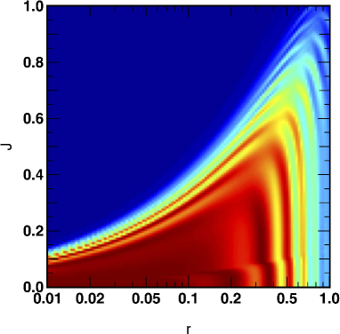
Figure 8: Comparison between the reflecting central sphere method (left panel) and our improved delayed central sphere implementation (right panel). A simulation of a Hénon sphere with $(N_{r},N_{v},N_{j})=(200,200,200)$ and a virial ratio $R=0.5$ is shown at $t=30$ in the $\left(r,u=0,j\right)$ plane. The systematic artificial speed increase undergone by orbits that penetrate the central region compared to their higher angular momentum counterparts can clearly be observed at low $j$ on the left panel where a reflective sphere is used, while the distribution function does not exhibit such spurious features when a delayed kernel is used (right panel).

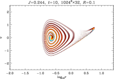
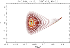
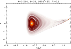
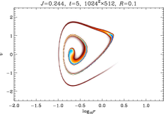
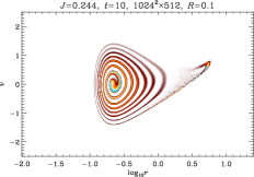
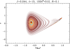
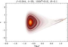
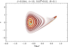
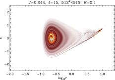
Figure 9: Effect of resolution in the Vlasov code: phase-space density for $R=0.1$ and $j=0.244$. Each column of panels corresponds to a given value of time $t$, increasing from left to right, while each line correspond to a given resolution, $(N_{r},N_{v},N_{j})=(2048,2048,32)$, $(1024,1024,32)$, $(1024,1024,512)$ and $(512,512,512)$ from top to bottom, as indicated on each panel. The pictures show only the $f\geq 0$ part of the phase-space density, while it can actually become negative because of aliasing. However, this choice of representation does not hide aliased regions. The prominent one corresponds to the textured zone above the large $r$ tail of the system on the right panels.

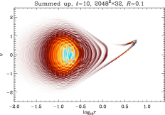
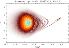
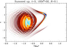
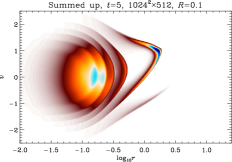
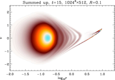
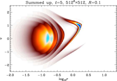
Figure 10: Same as in Fig. 9, but the phase-space distribution function has now been summed up over the whole available range of values of $j\in[0,J_{\rm max}=1.6]$, where $J_{\rm max}$ is the maximum sampled value of $j$.

In this appendix, we explain how reflecting boundaries conditions with time delay are implemented in VlaSolve.

If the mass inside the sphere of radius $R_{\rm min}$ is neglected, the trajectories followed by each test particle associated to a grid site that penetrates the sphere are fixed and do not depend on time. This property, combined with the fact that we use a constant time step, allows us to pre-compute these trajectories once and for all. The delayed central sphere method is then implemented by associating a linked list to each grid site whose associate test particle radial position $r$ half a time step backward in time is such that $r\leq R_{\rm min}$. Each linked list contains as many elements as the number of time steps needed for the particle to travel a distance of $2R_{\rm min}$ and the $n^{\rm th}$ element in the list stores the coordinates of the test particle $n$ time steps backward in time. Before starting the simulation, we initialize each element coordinate and the corresponding value of the initial distribution function. For each time step, the value of each element is then simply updated by assigning to it the value of its successor while the last element value, whose coordinates fall inside the computing domain, $r\geq R_{\rm min}$, is interpolated. A comparison of the results obtained with the reflective central sphere to our improved delayed central sphere is shown on figure 8. The improvements are unquestionable.

A.2 Parallelization issues

We implemented a hybrid shared and distributed memory version of VlaSolve via the OpenMP and MPI libraries, respectively.

Shared memory parallelism is relatively straightforward to achieve in the spherically symmetric case, by taking advantage of the fact that the angular momentum $j$ is a conserved quantity. Spline interpolations, which represent the most expensive part of the code, can thus be computed independently for each slice of constant $j$. We therefore easily reach an almost perfect parallelization up to a number of tasks equal to the grid resolution $N_{j}$ of angular momentum space, which is typically larger than the number of available cores on a shared memory system.

Distributed memory parallelization via MPI is not as simple. Indeed, spline interpolations are intrinsically non-local, which makes the parallelization along dimensions other than $j$ non trivial. Sticking with the trivial parallelization described above unfortunately limits the maximum total number of processes running in parallel to $N_{j}$, which is suboptimal. We overcome this limitation by performing MPI domain decomposition in $(r,v)$ space, following the approach of Crouseilles & al. (2009), who propose to localize the cubic spline interpolation to each domain by using Hermite boundary conditions between the domains with an ad hoc reconstruction of the derivatives.

A.3 Effects of resolution

Figures 9 and 10 show, respectively for $j=0.244$ and integrated over angular momentum, the phase-space distribution function measured in VlaSolve simulations with different resolutions. These simulations have been performed for a Hénon sphere with initial virial ratio $R=0.1$. Beside the very good global agreement between the various runs, these figures bring out three effects, which increase when the resolution of the phase-space grid is reduced:

• Diffusion smearing out fine details that build up in phase-space during the course of dynamics, for instance clearly visible when one compares top to bottom middle panels of Fig. 9. One concern with diffusion is that it might prevent the appearance of unstable modes. However, we did not perform any simulation in this work that would prove this.

• Aliasing due to artificial oscillations in the spline interpolation: for the problem studied here, aliasing becomes particularly visible after relaxation in the region above the large $r$ tail, but this does not have significant impact on the dynamics.

• Aliasing due to undersampling angular momentum space: it is visible at all times when one examines the phase-space distribution function integrated over angular momentum (top panels of Fig. 10) and can have dramatic consequences on the dynamics. The two top lines of panels of Fig. 9 and 10, corresponding to a sparse sampling in $j$ space with only 32 slices, indeed show the appearance of an instability, which presents, on the third column of these figures, the same pattern whether $(N_{r},N_{v})=(2048,2048)$ or $(1024,1024)$. This instability is not present in the simulations with higher resolution in $j$, as shown by the two bottom lines of panels. Note that the presence of this instability depends on initial conditions: for $R=0.5$, we did not notice it for the time coverage considered, $t\leq 100$ (upper line of panels of Figs. 2 and 3).

Appendix B $N$-body simulations: exploration of the control parameter space

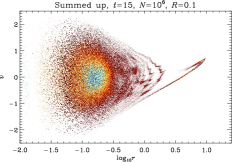
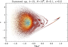
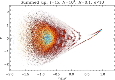
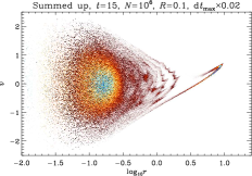
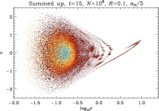
Figure 11: Effect of changing the important control parameters in Gadget. The phase-space density is shown at $t=15$ for Gadget simulations with the same initial conditions corresponding to the Hénon sphere with $R=0.1$ and involving $N=10^{6}$ particles. In each of the simulations, one control parameter was changed compared to the fiduciary simulation shown on left panel and which uses the settings of § 3. On top and bottom left panels, the softening length of the force was decreased by a factor 5 and increased by a factor 10, respectively. In top-right panel, the maximum possible time step was divided by a factor 50, while in the bottom-right panel, the tolerance parameter $\alpha_{\rm F}$ defined in § 3 was divided by a factor 5.

In § 5 we noticed the presence of an instability in the $R=0.1$ $N$-body simulations. One aim of this appendix is to confirm that this instability is related to the number of particles used in the simulations and not to any other control parameter of the Gadget code. In the same time, it is also an opportunity to check that our fiducial choice of the Gadget control parameters, given in § 3, is correct.

Figure 11 illustrates the main results of the tests we performed for simulations with $10^{6}$ particles. These tests consisted in changing the softening length of the force, the maximum time step value and the tolerance parameter $\alpha_{F}$ controlling the errors on the force. Improving the accuracy of the force calculation or dividing the maximum time step ${\rm d}t_{\rm max}$ by a factor 50, which corresponds to imposing ${\rm d}t\leq 2\times 10^{-4}$, does not change the results. This is confirmed as well by the measurements of the correlators $C_{k}$ introduced in § 6, that we do not show here for simplicity. Only the value of the softening parameter of the force $\epsilon$ has an impact on the dynamics for the tests we did. Reducing $\epsilon$ by a factor 5 seems to slightly blur the phase-space density, although this effect is difficult to decipher, while increasing $\epsilon$ by a factor 10 sharpens the fine structures of the phase-space density. Since $\epsilon$ controls the intensity of close encounters between particles, this is not surprising. Note that increasing $\epsilon$ by a factor 10 is probably an exaggeration, because it worsens dramatically the match during the mixing phase between the $N$-body simulation and the Vlasov code when examining the correlators $C_{k}$, a sign that $\epsilon$ is probably getting too close to a physical characteristic scale of the system. We indeed noticed that increasing $\epsilon$ only by a factor 5 does not have much impact, on the other hand, on $C_{k}$. However, all these effects do not affect the amplitude of the large scale irregularities on the pattern of $f(r,v,j)$, which are present whatever value of $\epsilon$. This is also a strong indication that close particle encounters are not at the origin of these irregularities.

We can therefore only conclude that these irregularities and the associated nonlinear instability are the result of non trivial collective effects related to particle shot noise. This argument is also supported by the fact that in addition, the moment of their appearance is particle number dependent, as discussed in § 5.

References

- Aarseth, Lin, & Papaloizou (1988) Aarseth S. J., Lin D. N. C., Papaloizou J. C. B., 1988, ApJ, 324, 288
- Alard & Colombi (2005) Alard C., Colombi S., 2005, MNRAS, 359, 123
- Barnes, Lanzel, & Williams (2009) Barnes E. I., Lanzel P. A., Williams L. L. R., 2009, ApJ, 704, 372
- Bertschinger (1998) Bertschinger E., 1998, ARA&A, 36, 599
- Besse & Sonnendrücker (2003) Besse N., Sonnendrücker E., 2003, JCoPh, 191, 341
- Besse et al. (2008) Besse N., Latu G., Ghizzo A., Sonnendrücker E., Bertrand P., 2008, JCoPh, 227, 7889
- Binney (2004) Binney J., 2004, MNRAS, 350, 939
- Boily, Athanassoula, & Kroupa (2002) Boily C. M., Athanassoula E., Kroupa P., 2002, MNRAS, 332, 971
- Campos Pinto (2011) Campos Pinto M., 2011, arXiv, arXiv:1112.1859
- Cheng & Knorr (1976) Cheng C. Z., Knorr G., 1976, JCoPh, 22, 330
- Colombi (2001) Colombi S., 2001, NewAR, 45, 373
- Colombi & Touma (2008) Colombi S., Touma J., 2008, CNSNS, 13, 46
- Colombi & Touma (2014) Colombi S., Touma J., 2014, MNRAS, 441, 2414
- Crouseilles & al. (2009) Crouseilles N., Latu G., Sonnendrücker, E., 2009, JCoPh, 228, 1429
- Crouseilles, Mehrenberger, & Sonnendrücker (2010) Crouseilles N., Mehrenberger M., Sonnendrücker E., 2010, JCoPh, 229, 1927
- Dehnen & Read (2011) Dehnen W., Read J. I., 2011, EPJP, 126, 55
- Dolag et al. (2008) Dolag K., Borgani S., Schindler S., Diaferio A., Bykov A. M., 2008, SSRv, 134, 229
- Filbet, Sonnendrücker, & Bertrand (2001) Filbet F., Sonnendrücker E., Bertrand P., 2001, JCoPh, 172, 166
- Fujiwara (1981) Fujiwara T., 1981, PASJ, 33, 531
- Fujiwara (1983) Fujiwara T., 1983, PASJ, 35, 547
- Gott (1973) Gott, J.R. III , 1973, ApJ, 186, 481
- Güçlü, Christlieb, & Hitchon (2014) Güçlü Y., Christlieb A. J., Hitchon W. N. G., 2014, JCoPh, 270, 711
- Hahn, Abel, & Kaehler (2013) Hahn O., Abel T., Kaehler R., 2013, MNRAS, 434, 1171
- Hallé (2015) Hallé A., 2015, private communication
- Hénon (1964) Hénon M., 1964, AnAp, 27, 83
- Henriksen & Widrow (1997) Henriksen R. N., Widrow L. M., 1997, PhRvL, 78, 3426
- Hozumi, Burkert, & Fujiwara (2000) Hozumi S., Burkert A., Fujiwara T., 2000, MNRAS, 311, 377
- Hozumi, Fujiwara, & Kan-Ya (1996) Hozumi S., Fujiwara T., Kan-Ya Y., 1996, PASJ, 48, 503
- Huss, Jain, & Steinmetz (1999) Huss A., Jain B., Steinmetz M., 1999, ApJ, 517, 64
- Jing & Suto (2000) Jing Y.P., Suto, Y., 2000, ApJL, 529, L69
- Jing & Suto (2002) Jing Y.P., Suto, Y., 2002, ApJ, 574, 538
- Joyce, Marcos, & Sylos Labini (2009) Joyce M., Marcos B., Sylos Labini F., 2009, MNRAS, 397, 775
- Melott (2007) Melott A. L., 2007, arXiv, arXiv:0709.0745
- Melott et al. (1997) Melott A. L., Shandarin S. F., Splinter R. J., Suto Y., 1997, ApJ, 479, L79
- Mineau, Feix, & Rouet (1990) Mineau P., Feix M. R., Rouet J. L., 1990, A&A, 228, 344
- Moore et al. (1998) Moore B., Governato F., Quinn T., Stadel J., Lake G., 1998, ApJ, 499, L5
- Nishida et al. (1981) Nishida M. T., Yoshizawa M., Watanabe Y., Inagaki S., Kato S., 1981, PASJ, 33, 567
- Power et al. (2003) Power C., Navarro J. F., Jenkins A., Frenk C. S., White S. D. M., Springel V., Stadel J., Quinn T., 2003, MNRAS, 338, 14
- Rossmanith & Seal (2011) Rossmanith J. A., Seal D. C., 2011, JCoPh, 230, 6203
- Roy & Perez (2004) Roy F., Perez J., 2004, MNRAS, 348, 62
- Shandarin, Habib, & Heitmann (2012) Shandarin S., Habib S., Heitmann K., 2012, PhRvD, 85, 083005
- Shoucri & Gagne (1978) Shoucri M. M., Gagne R. R. J., 1978, JCoPh, 27, 315
- Sonnendrücker et al. (1999) Sonnendrücker E., Roche J., Bertrand P., Ghizzo A., 1999, JCoPh, 149, 201
- Splinter et al. (1998) Splinter R. J., Melott A. L., Shandarin S. F., Suto Y., 1998, ApJ, 497, 38
- Springel (2005) Springel V., 2005, MNRAS, 364, 1105
- Springel et al. (2008) Springel V., et al., 2008, MNRAS, 391, 1685
- Springel, Yoshida, & White (2001) Springel V., Yoshida N., White S. D. M., 2001, NewA, 6, 79
- Stadel et al. (2009) Stadel J., Potter D., Moore B., Diemand J., Madau P., Zemp M., Kuhlen M., Quilis V., 2009, MNRAS, 398, L21
- Sylos Labini (2012) Sylos Labini F., 2012, MNRAS, 423, 1610
- Umeda (2008) Umeda T., 2008, EP&S, 60, 773
- van Albada (1982) van Albada T. S., 1982, MNRAS, 201, 939
- Watanabe et al. (1981) Watanabe Y., Inagaki S., Nishida M. T., Tanaka Y. D., Kato S., 1981, PASJ, 33, 541
- Yoshikawa, Yoshida, & Umemura (2013) Yoshikawa K., Yoshida N., Umemura M., 2013, ApJ, 762, 116