A Method for the Estimation of p-Mode Parameters from Averaged Solar Oscillation Power Spectra

Abstract

A new fitting methodology is presented which is equally well suited for the estimation of low-, medium-, and high-degree mode parameters from $m$-averaged solar oscillation power spectra of widely differing spectral resolution. This method, which we call the “Windowed, MuLTiple-Peak, averaged spectrum”, or WMLTP Method, constructs a theoretical profile by convolving the weighted sum of the profiles of the modes appearing in the fitting box with the power spectrum of the window function of the observing run using weights from a leakage matrix that takes into account both observational and physical effects, such as the distortion of modes by solar latitudinal differential rotation. We demonstrate that the WMLTP Method makes substantial improvements in the inferences of the properties of the solar oscillations in comparison with a previous method that employed a single profile to represent each spectral peak. We also present an inversion for the internal solar structure which is based upon 6,366 modes that we have computed using the WMLTP method on the 66-day long 2010 SOHO/MDI Dynamics Run. To improve both the numerical stability and reliability of the inversion we developed a new procedure for the identification and correction of outliers in a frequency data set. We present evidence for a pronounced departure of the sound speed in the outer half of the solar convection zone and in the subsurface shear layer from the radial sound speed profile contained in Model S of Christensen-Dalsgaard and his collaborators that existed in the rising phase of Solar Cycle 24 during mid-2010.

1 Introduction

Helioseismology provides a unique opportunity to investigate in great detail the internal structure and rotation of the Sun. The starting point for the study of the solar interior using helioseismology can be identified with the observational confirmation by Deubner (1975), and independently by Rhodes et al. (1977), of the standing-wave nature of the solar five-minute oscillations that were observed in the solar photosphere as proposed by Ulrich (1970), and independently by Leibacher & Stein (1971). The remarkable qualitative agreement of the observations of Deubner (1975) and of Rhodes et al. (1977) with the predictions of the theoretical studies meant that the five-minute oscillations could be regarded as a superposition of acoustic normal modes that are trapped in the interior of the Sun. However, the frequencies of the observed ridges of power in the dispersion plane were systematically lower by about 5 % than the theoretical predictions. This discrepancy allowed Rhodes et al. (1976), and independently Gough (1977) to provide observational estimates of the depth of the solar convection zone. These estimates are now believed to be the first helioseismic inferences of solar internal structure.

The observed modes are predominantly $p$-modes, for which pressure provides the dominant restoring force. Also observed is the $f$-mode, which at high spherical harmonic degree $l$ has the character of a surface gravity wave. Both the Deubner (1975) and Rhodes et al. (1977) studies employed intermediate- and high-degree $f$- and $p$-modes, while Claverie et al. (1979) employed low-degree $p$-modes that penetrated into the solar core. Today, the line of demarcation between low- and intermediate-degree modes is at $l=4$ (the highest degree that can be observed in integrated light), while that between intermediate- and high-degree modes is where individual modes are no longer resolved, or at about $l=300$ for the $f$-mode, between $l=200$ and $l=150$ for the $n=1$ through $n=4$ ridges (and at lower values of $l$ for the higher radial orders $n$).

The observations by Deubner (1975), Rhodes et al. (1977), and Claverie et al. (1979) raised considerable debate over the proper characterization of the oscillation modes that had been observed. Deubner (1977) cited a pre-publication version of Deubner et al. (1979) to claim that the solar $p$-mode oscillations were truly global in nature, but subsequently, Ulrich et al. (1979) disagreed with this conclusion and argued that “…the modes of greatest interest are not globally coherent because of the effect of convective motions associated with the supergranulation”. Furthermore, Hill (1980) and Gough (1980) pointed out that the coherence times of up to nine hours that were cited by Deubner et al. (1979) and by Claverie et al. (1980) were not sufficient to demonstrate the global nature of these modes. Today, the term “global helioseismology” refers either to studies that employ the low- and intermediate-degree $p$-modes whose lifetimes are truly long enough for them to be globally-coherent or to studies that employ spherical harmonic decompositions that are computed from nearly the entire visible solar hemisphere. Studies that do not use modes which have such long lifetimes or which are computed from observations that cover much smaller portions of the visible hemisphere are considered to employ the tools of “local helioseismology”.

Depending on the frequency and degree $l$, the modes propagate within different acoustic cavities inside the Sun between two turning points. Outside the acoustic cavity in which a mode is propagating, the mode is evanescent. Therefore, the mode characteristics (e.g., frequency) are relatively insensitive to conditions outside the associated acoustic cavity, particularly far from the turning points. Moreover, modes which propagate in the direction of solar rotation have higher frequencies than modes with the same resonant properties propagating in the opposite direction. This effect is called “rotational frequency splitting”. The amount of splitting depends on the rotation rate inside the acoustic cavity in which the mode is propagating as well as on the azimuthal order $m$ of the mode. Utilizing the differential penetration and the frequency splitting of the modes allows the internal structure and rotation of the Sun to be inferred, as a function of position (cf. Christensen-Dalsgaard, 2002). This possibility of carrying out inversions of the observed frequencies and frequency splittings is a key issue in the applications of helioseismology. So far, however, the vast majority of inversions performed have only included frequencies and frequency splittings of the low- and the intermediate-degree oscillations (see, e.g., Gough et al., 1996; Thompson et al., 1996; Antia & Chitre, 1998; Kosovichev et al., 1998; Schou et al., 1998). On the other hand, high-degree $f$- and $p$-modes have an immense potential in the helioseismic probing of the sub-surface layers of the Sun. This is demonstrated here in Figure 1, where the dependence of the inner turning-point radius $r_{\rm t}$ on spherical harmonic degree $l$ is shown for three different frequencies, spanning the range of the observations. For small $l$, the inner turning point is rather close to the center of the Sun, whereas for higher degrees it moves closer to the surface. In particular, for $l>150$ the modes are essentially trapped in the outer 65 Mm below the solar surface. Therefore, accurate measurements of high-degree mode frequencies and splittings allow us to improve our inferences regarding the large-scale structure and dynamics of the sub-surface layers (see, e.g., Rabello-Soares et al., 2000, 2008a; Di Mauro et al., 2002).

Figure 1: Location $r_{\rm t}$ of the inner turning point (a), and depth of penetration $R-r_{\rm t}$ (b), in units of the solar radius $R$, for $p$-modes in a standard solar model. The results are shown as functions of degree $l$, for three typical frequencies. Adapted from Christensen-Dalsgaard (2003).

Due to the use of a modal concept in global helioseismology, the diagnostic potential of the data is necessarily limited. Specifically, to first order the standing acoustic modes sense only the longitudinally averaged, north-south symmetric average of the internal stratification of the Sun. Moreover, in contrast to solar differential rotation, flows in meridional planes (meridional circulation) have only a tiny effect on global oscillation frequencies (Woodard, 2000; Roth & Stix, 2008; Schad et al., 2011; Vorontsov, 2011; Schad et al., 2013), which severely hampers any attempt to detect such flows by global mode frequency analysis. Such limitations are avoided in local helioseismology, which is based upon the assumption that the solar oscillations locally behave as propagating acoustic waves that are scattered and absorbed by local inhomogeneities and advected by local flow fields. Braun et al. (1987) were the first to demonstrate the utility of this approach by showing that propagating acoustic waves could be absorbed by the strong magnetic field associated with sunspots, thus potentially providing information about the magnetic field itself. Subsequently, three methods of analyzing propagating acoustic waves in a localized area on the solar surface were devised: ring-diagram analysis (Hill, 1988; González-Hernández, 2008), time-distance analysis (Duvall et al., 1993; Kosovichev, 1996b; Gizon & Birch, 2005; Zhao, 2004, 2008), and acoustic holography (Lindsey & Braun, 2000, 2004). The application of these methods has led to spectacular results, as has been demonstrated by, e.g., Giles et al. (1997), Kosovichev et al. (2000), Braun & Lindsey (2001), Beck et al. (2002), Haber et al. (2002). For a review of local helioseismology we refer the reader to Gizon et al. (2010).

While in recent years the progress made in local helioseismology has been substantial, it has been much slower in global helioseismology. This is in part a consequence of the difficulties inherent in the generation of reliable high-degree mode parameters, but misconceptions as to the roles of local and global helioseismology may have contributed as well. One such misconception is that the global mode measurements can be replaced with measurements from local analyses. As Reiter (2007) has demonstrated, at large-scales the local measurements are much less precise than the global measurements and, therefore, there is a strong complementarity between the local and global techniques.

The estimation of high-degree mode parameters is made difficult due to the fact that high-degree modes cannot be observed as sharp, isolated peaks but only as ridges of power comprised of overlapping modes. Because of the asymmetrical distribution of the amplitudes of the modes that blend together, the central frequency of each ridge deviates from the frequency of the target mode. Hence, to recover the underlying mode frequency from fitting the ridge, an accurate model of the ridge power as a function of frequency is required. With such an accurate model the global analysis provides the most robust estimates of the mean structure and rotation of the Sun which are important for testing theories of stellar structure, evolution, and differential rotation.

We began to delve into the fitting of solar oscillation spectra in the late-1980s with the development of our first-generation, or Single-Peak, Averaged-Spectrum, fitting method, which we will refer to in the following as either Method 1 or the SPAS method, and which is briefly described here in Appendix A. Because of insurmountable problems with the determination of unbiased ridge-fit frequencies we had to abandon this method, however. We therefore began to develop our second-generation, or Windowed, MuLTiple-Peak, averaged-spectrum, fitting method, which we will refer to in the following as either Method 2 or the WMLTP method. This method is equally well suited for the unbiased estimation of low-, medium-, and high-degree mode parameters from $m$-averaged solar oscillation power spectra. A detailed description of this method will be presented in Section 4, after we have given an outline of the data analysis generally employed in global helioseismology in Section 2, and after we have addressed the problems inherent in the analysis of high-degree power spectra in Section 3. The issue of the sensitivity of Method 2 in terms of both the $m$-averaging procedure and the effective leakage matrix is addressed in Section 5. Sample results from Method 2 are presented in Section 6. In Section 6 we will also demonstrate the substantial improvements that Method 2 makes in the frequencies, linewidths, and amplitudes that we generated with this method by comparing them with corresponding quantities that we generated using our Method 1. Finally, in Section 7 we firstly describe a new procedure for the identification and correction of outliers in frequency data sets that are to be used for solar structure inversions, before we present a new structural inversion from a set of frequencies computed from 66-day long spectra obtained with the Michelson Doppler Imager (MDI) (Scherrer et al., 1995) on board the SOlar and Heliospheric Observatory (SOHO) (Domingo et al., 1995) at the beginning of solar cycle 24 in 2010, followed by our concluding remarks in Section 8.

At this point we note that the current paper is the first of a series of three papers. While the focus of the paper at hand is on Method 2, we will present in the second paper our third-generation, or Multiple-Peak, Tesseral-Spectrum, fitting method, which we will refer to in the following as either Method 3 or the MPTS method. This method directly fits the tesseral, zonal, and sectoral spectra at each degree rather than resorting to $m$-averaged spectra as is the case with both Method 1 and 2. In that paper we will also intercompare the results obtained from Method 2 and 3, and we will investigate the systematic effects introduced in Method 2 by the $m$-averaging procedure. The purpose of the third paper will be the intercomparison of our results obtained from both Method 2 and 3 with results from “established” fitting methodologies at low, intermediate, and high degrees.

2 Data analysis in global helioseismology

In global helioseismic studies the data reduction typically includes the following major steps. First, the observed Dopplergrams $V(\theta,\phi,t)$ are spatially decomposed into spherical harmonic coefficients $\mathfrak{a}_{l,m}(t)$, i.e.,

$$\mathfrak{a}_{l,m}(t)=\int_{\mathcal{D}}W(\theta,\phi)V(\theta,\phi,t)Y_{l}^{m}(\theta,\phi)\,\mathrm{d}\sigma,$$ (1)

where $\theta$ is co-latitude, $\phi$ is longitude, $Y_{l}^{m}(\theta,\phi)$ is a spherical harmonic function of degree $l$ and azimuthal order $m$, $W(\theta,\phi)$ is an apodization chosen to reduce the contribution from the noise close to the solar limb, $\mathcal{D}$ is the visible hemisphere of the Sun or a portion thereof, and $t$ is time. In this step of the data reduction spatial side-lobes are introduced into the target spectrum $(l,m)$ because the spherical harmonic functions $Y_{l}^{m}(\theta,\phi)$ are not orthogonal on $\mathcal{D}$. However, even if the entire surface of the Sun could be observed spatial side-lobes would be present because of the distortion of the mode eigenfunctions by solar latitudinal differential rotation, and also because of velocity projection effects. The integral in equation (1) can be very expensive to compute. A typical approach is to use interpolation to remap, for given time $t$, the product $W(\theta,\phi)V(\theta,\phi,t)$ onto some coordinate system in which the integration over $\phi$ may be represented as a Fourier transform, so that Fast Fourier Transform (FFT) techniques may be applied. In the second step a spectral analysis is carried out for each spherical harmonic coefficient $\mathfrak{a}_{l,m}(t)$, i.e.,

$$\mathfrak{A}_{l,m}(\nu)=\int_{-\infty}^{+\infty}\mathfrak{a}_{l,m}(t)\exp(2\pi i\nu t)\,\mathrm{d}t,$$ (2)

where $\nu=\omega/2\pi$ is cyclic frequency. In this step temporal side-lobes are introduced into the target spectrum $(l,m)$ if periodic gaps are present in the time series of the spherical harmonic coefficients $\mathfrak{a}_{l,m}(t)$ due to the day-night cycle, say. In practice, the integral in equation (2) is first approximated by a discrete Fourier transform over a finite interval of time, which then is efficiently computed using a FFT technique. In the third step the power spectrum $\Phi_{l,m}(\nu)=|\mathfrak{A}_{l,m}(\nu)|^{2}$ is calculated for each $(l,m)$. The final step in the data reduction consists in the peak fitting of the power spectra $\Phi_{l,m}(\nu)$. Alternatively, the peaks in the complex spectra $\mathfrak{A}_{l,m}(\nu)$ can be fitted as well. For example, such approach is employed in the fitting methodology of Schou (1992).

2.1 Generation of un-averaged power spectra

The results presented in this investigation are based upon four different sets of un-averaged power spectra $\Phi_{l,m}(\nu)$ that were created from observations obtained with the MDI instrument during 1996, 2001 and 2010. The MDI was operated on the SOHO spacecraft between April 1996 and April 2011. The MDI observations which we have employed were all obtained as part of the MDI Full-Disk Program (Scherrer et al., 1995), and are listed in Table 1, where we also indicate the naming convention we use in this paper to refer to each observing run.

Time series of Dopplergrams that resulted from each of the four observing runs listed in Table 1 were converted into $l+1$ complex time series (purely real for $m=0$) which were gap-filled using an auto-regressive gap filling procedure based upon the approach of Fahlman & Ulrych (1982), using a reduction pipeline that was developed at Stanford University for the processing of the MDI data. The resulting gap-filled duty cycles are listed in the last column of Table 1. Using standard FFT techniques the gap-filled $l+1$ complex time series were converted into a group of $2l+1$ zonal, tesseral, and sectoral power spectra for $0\leq l\leq 1000$ for each of the four observing runs. In doing so, the positive frequency part is identified with $m<0$, while the negative frequency part is identified with $m\geq 0$.

Within each of these four groups of un-averaged power spectra, each target spectrum $(l,m)$ contains a number of frequency bins equal to one-half of the number of samples that is listed in the corresponding row of column 3 in Table 1. For the MDI instrument, these frequency bins span the frequency range of zero to the temporal Nyquist frequency of $8333\,\,\mu$Hz. Within each group of spectra the zonal (i.e., $m=0$) spectrum for a given degree, $l$, contains a variable number of sets of isolated peaks (at low- and intermediate degrees) or a set of ridges (at higher degrees) of power that correspond to a collection of $f$- and $p$-modes. For the cases in which the peaks are isolated, each set of peaks consists of a peak for the target mode $(n,l)$, the set of temporal sidelobes, and a set of spatial sidelobes that have leaked into the target spectrum from nearby spectra. We will refer to the entire collection of $2l+1$ target peaks and their spatial and temporal sidelobes that share a common $n$-value as the $(n,l)$ multiplet. When we refer to the mode $(n,l)$, we are actually referring to the $m$-average of the $2l+1$ modes that share the same values of $n$ and $l$.

For the tesseral and sectoral spectra the corresponding peaks in each spectrum are shifted to lower frequencies by solar rotation for the spectra having $m<0$, while they are shifted to higher frequencies for the spectra having $m>0$ (cf. Christensen-Dalsgaard et al., 2000).

2.2 Procedures for the generation of m-averaged power spectra

For a given degree, $l$, the $m$-averaged power spectrum $\Phi_{l}^{\mathrm{mav}}(\nu)$ is defined as

$$\Phi_{l}^{\mathrm{mav}}(\nu)=\langle\Phi_{l,m}(\nu)\rangle_{m},$$ (3)

where the symbol $\langle\,\rangle_{m}$ means averaging over $m$, is computed in a three-step procedure. In the first step of this procedure, the frequency shift resulting from the effect of solar rotation and asphericity is calculated, for each of the $2l+1$ un-averaged spectra, $\Phi_{l,m}(\nu)$, using an iterative cross-correlation method (Brown, 1985; Tomczyk, 1988; Korzennik, 1990). In this method the frequencies within a multiplet $(n,l)$ are approximated with a polynomial expansion similar to that of Duvall et al. (1986), i.e.,

$$\nu_{n,l,m}=\nu_{n,l}+L\sum_{k=1}^{6}a^{(n,l)}_{k}P_{k}(m/L).$$ (4)

Here, $\nu_{n,l}$ is the frequency of the multiplet $(n,l)$, $L^{2}=l(l+1)$, $a^{(n,l)}_{k}$ are the so-called frequency-splitting coefficients, and $P_{k}$ is the Legendre polynomial of degree $k$. The splitting coefficients $a^{(n,l)}_{k}$ with odd $k$ arise from solar internal rotation, while the coefficients with even $k$ are caused by departures from spherical symmetry in solar structure, or from effects of magnetic fields. Most of the $m$-averaged power spectra that we fit for this manuscript were generated using only the three lowest, odd-$k$ frequency-splitting coefficients (i.e., $a_{1}$, $a_{3}$, and $a_{5}$). In the second step of the process in which we computed the $m$-averaged spectra, we shifted each tesseral and sectoral spectrum by the calculated frequency shift for that $m$-value. In the third step in this procedure, we averaged all of these shifted spectra together with the un-shifted zonal spectrum, $\Phi_{l,0}(\nu)$, to create the $m$-averaged spectrum $\Phi_{l}^{\mathrm{mav}}(\nu)$ for each degree $l$. If this $m$-averaging is carried out in an unweighted manner, we will refer to the resulting set of $m$-averaged spectra as “unweighted, $m$-averaged spectra”. However, as we previously described in Rhodes et al. (2001), it is also worth considering average spectra computed by combining the $2l+1$ spectra $\Phi_{l,m}(\nu)$ in a weighted manner, using as weights the inverse mean power over the 1500 to $4500\,\,\mu$Hz frequency range. We will refer to such a set of spectra as “weighted, $m$-averaged spectra”.

We have developed two different versions of the cross-correlation method to generate rotational splitting coefficients which then are used in the computation of the $m$-averaged spectra. In the first of these versions, we cross-correlate the individual spectra over a wide range of frequencies such that most or all of the ridges at a given degree are included, while in the second version we carry out the cross-correlation over a narrow range of frequencies centered about a single ridge at each degree. In the second version, we then repeat these narrow-band cross-correlations for all of the successive ridges at a given degree in order to build up a set of narrow-band splitting coefficients for that degree. In the wide-band version of the cross-correlation code we effectively are computing the averages of the frequency splittings over all of the adjacent ridges which are located within the frequency limits of the cross correlation (typically from 1800 to $4800\,\,\mu$Hz). The splitting coefficients from the wide-band procedure are called the $n$-averaged splitting coefficients, while those from the narrow-band version of our code are called non-$n$-averaged splitting coefficients.

2.3 Correction for distortions introduced by latitudinal differential rotation

For the results that we will be presenting later, we generated a set of $n$-averaged frequency-splitting coefficients by cross-correlating the un-averaged power spectra obtained from the $\cal{R}$1996_61 observing run (cf. Table 1). The odd-order splitting coefficients (i.e., $a_{1}$, $a_{3}$, and $a_{5}$) that we obtained from this procedure are shown here in the left three panels of Figure 2. These raw frequency-splitting coefficients show large discontinuities in the degree range of $200\lesssim l\lesssim 240$. Similar discontinuities were first noticed by Korzennik (1990). Subsequently, Rhodes et al. (1998a) confirmed the presence of these jumps in MDI observations. The exact location of the range of $l$ values where these jumps occur depends primarily upon the duration of the observing run from which the power spectra were generated, with shorter-duration observing runs showing the jumps at lower degrees.

Figure 2: (left) Degree dependence of the $n$-averaged odd-order splitting coefficients $a_{1}$, $a_{3}$, and $a_{5}$, in the range $5\leq l\leq 1000$ computed from the set of un-averaged power spectra obtained from the $\cal{R}$1996_61 observing run, with the $a_{1}$ coefficient at the top. As can be clearly seen, these raw splitting coefficients illustrate large discontinuities at about $l\approx 210$. (right) Same as shown in the left panels, but after the discontinuities have been removed using the adjustment procedure described in Section 2.2.

Woodard (1989) pointed out that the distortion of high-degree $f$- and $p$-mode eigenfunctions caused by a slow, antisymmetric differential rotation can be expressed as a superposition of the unperturbed eigenfunctions of the same radial order $n$ if the Coriolis forces are neglected. Following a discussion of Woodard’s suggestion in a preprint of Korzennik et al. (2004), Reiter et al. (2003) found that the inclusion of this effect in the calculation of the leakage matrices had a very dramatic impact upon the resulting frequency-splitting coefficients. Examples of the changes introduced into the odd splitting coefficients when corrections are made for the distortion were presented by Reiter et al. (2003), who showed that at the degrees below $l\approx 200$ the splitting coefficients remained almost unchanged, while at the higher degrees the jumps were seen to disappear when the mode coupling due to the differential rotation of the Sun was taken into account.

The results that Reiter et al. (2003) presented were generated using a preliminary version of our MPTS method that we have been developing in parallel to the WMLTP method that we are presenting in this paper. Because: 1) the MPTS method is extremely computationally-intensive; 2) it cannot be employed upon power spectra that come from observing runs that are as short as only three days in duration due to the low signal-to-noise ratios that are inherent in such low-resolution spectra; and 3) we have not yet had the opportunity of implementing the changes that we have recently made in our WMLTP method into the MPTS code, we have not yet employed the MPTS method to compute entire sets of frequency-splitting coefficients. Instead, we corrected the raw splitting coefficients that are shown in the left three panels of Figure 2 with a two-step adjustment procedure. First, for each of the five splitting coefficients we fit a least-squares straight line to the degree range of 90 to 190 and we also fit a second least-squares straight line to the degree range from 230 to 400. For the degrees ranging from 200 to 230 the two linear fits for each splitting coefficient were simply connected with a third straight line. The difference between that line and the extrapolation of the left-hand line was subtracted from the raw coefficient values for all of the degrees between 200 and 230. For all degrees above $l=230$ the offset employed for $l=230$ was subtracted from each coefficient. Because these initially-corrected splitting coefficients showed evidence of systematic variations with increasing degree in the three odd-order coefficients (i.e., $a_{1}$, $a_{3}$, and $a_{5}$), we computed, in the second step of our correction procedure, a low-order polynomial fit to each of the three odd-order coefficients over the degree range of 488 to 1000. We then subtracted these polynomial fits from the partially-corrected, odd-order splitting coefficients and we stopped the correction process at this point. This procedure generated the set of corrected odd-order splitting coefficients that are shown in the right three panels of Figure 2, where it is clear that the jumps have been removed. We refer to this set of adjusted frequency-splitting coefficients as our set of “corrected, $n$-averaged” coefficients.

Using a similar adjustment procedure we also have corrected the set of raw non-$n$-averaged frequency-splitting coefficients that we previously computed using the narrow-band version of our cross-correlation method on the un-averaged power spectra obtained from the $\cal{R}$1996_61 observing run. We refer to this set of adjusted frequency-splitting coefficients as our set of “corrected, non-$n$-averaged” coefficients.

2.4 Sets of m-averaged power spectra generated from the observing runs used in this work

From the un-averaged power spectra obtained from the observing runs specified in Table 1 we have generated a total of seven different sets of $m$-averaged power spectra, which are listed in the second column of Table 2 using a naming convention quite similar to that introduced in Table 1 to refer to the individual observing runs. These seven sets of $m$-averaged spectra differed in four key ways: 1) origin of the un-averaged power spectra, 2) whether or not the raw, un-averaged spectra were weighted prior to being averaged, 3) whether the set of frequency-splitting coefficients was used as computed or as corrected for the effects of latitudinal differential rotation and other features that appeared not to be solar in origin, and 4) whether or not the set of frequency-splitting coefficients was computed using a narrow or a wide frequency range at each degree (i.e., whether those coefficients were computed for the individual ridges or were computed in an $n$-averaged manner). We note that we will not present any fits to the $m$-averaged spectral set $\cal{S}$1996_61 in this work. Rather, this set of $m$-averaged spectra is listed in Table 2 only for the sake of completeness because it was a by-product of the cross-correlation process that generated the raw, uncorrected, $n$-averaged splitting coefficients from observing run $\cal{R}$1996_61.

3 Problems requiring the use of multiple peaks in the fitting profile

3.1 Basic considerations

For the following reasons, high-degree modes cannot be observed as isolated, sharp peaks but only as ridges of power. First, the power spectrum computed for a specific target mode with degree $l$ and azimuthal order $m$ contains contributions of power from modes with neighboring $l$ and $m$ because the spherical harmonic functions used in the spatial decomposition of the observed Dopplergrams are not orthogonal on that part of the Sun we observe (see equation (1)). These unwanted contributions, or spatial leaks, are quantified by the so-called leakage matrix (see Sect. 3.2). Second, with increasing degree the frequency separation of the spatial leaks decreases, while the mode linewidth increases with both frequency and degree. As a consequence, individual modal peaks blend together to form ridges of power. Typically, modes begin to blend into ridges for degrees ranging anywhere from $l\approx 20$ ($n=29$) to $l\approx 300$ ($n=0$) depending on the radial order $n$. Since the amplitudes of the spatial leaks are asymmetric with regard to the target mode the central frequency of a ridge is significantly offset from the target mode frequency. Therefore, the distribution of power in a ridge cannot be simply represented by using just a single symmetrical or asymmetrical function of frequency. Rather, a sum of individual overlapping profiles must be employed the relative amplitudes of which are governed by the leakage matrix appropriate to the targeted mode. Thus, the correct estimation of the leakage matrix is crucial in the accurate measurement of high-degree mode parameters. Moreover, the use of a model profile consisting of the sum of individual profiles allows the fitting of low-, medium-, and high-degree modes in like manner. In this way systematic errors are avoided which otherwise would be inevitably introduced if subsets of mode parameters are to be combined each of which has been generated by using a different fitting methodology.

3.2 Leakage matrix

While the determination of the leakage matrix is straightforward for low- and medium-degrees, at high degrees the leakage matrix calculations are greatly complicated by the necessity to take into account (1) the horizontal component velocity, (2) the distortion of the eigenfunctions by the solar differential rotation, and (3) instrumental effects that cause image distortion and smearing. We will address these issues in the following paragraphs.

3.2.1 Radial and horizontal component

The Fourier transform $\tilde{O}_{l,m}$ of the time series of spherical harmonic amplitudes of a target mode with degree $l$ and azimuthal order $m$ can be written as a sum over the Fourier transform $\tilde{o}_{n^{\prime},l^{\prime},m^{\prime}}$ of the time series of the solar oscillation modes given by $(n^{\prime},l^{\prime},m^{\prime})$, viz.

$$\tilde{O}_{l,m}=\sum_{n^{\prime},l^{\prime},m^{\prime}}C_{n^{\prime};l,m;l^{\prime},m^{\prime}}\,\tilde{o}_{n^{\prime},l^{\prime},m^{\prime}},$$ (5)

where $C_{n^{\prime};l,m;l^{\prime},m^{\prime}}$ is the leakage matrix. As Korzennik et al. (2004) have shown, the leakage matrix can be written as

$$C_{n^{\prime};l,m;l^{\prime},m^{\prime}}=C_{l,m;l^{\prime},m^{\prime}}^{\,\mbox{\scriptsize(r)}}+c_{t}^{(n^{\prime},l^{\prime})}C_{l,m;l^{\prime},m^{\prime}}^{\,\mbox{\scriptsize(h)}},$$ (6)

where $C_{l,m;l^{\prime},m^{\prime}}^{\,\mbox{\scriptsize(r)}}$ is the part coming from the radial displacement, $C_{l,m;l^{\prime},m^{\prime}}^{\,\mbox{\scriptsize(h)}}$ is the part coming from the horizontal displacement, and $c_{t}^{(n^{\prime},l^{\prime})}$ is the ratio of the horizontal displacement to the radial displacement. It should be noted that both $C_{l,m;l^{\prime},m^{\prime}}^{\,\mbox{\scriptsize(r)}}$ and $C_{l,m;l^{\prime},m^{\prime}}^{\,\mbox{\scriptsize(h)}}$ are independent of the radial order $n^{\prime}$ of the mode. Using the normalization of the displacement eigenfunction components given by Gough (1993), the displacement component ratio is given by

$$c_{t}^{(n,l)}=\frac{|\xi_{n,l}^{\,\mbox{\scriptsize(h)}}(r_{\ast})|}{|\xi_{n,l}^{\,\mbox{\scriptsize(r)}}(r_{\ast})|}.$$ (7)

Here, $r_{\ast}$ is the radial location of observation, and $\xi_{n,l}^{\,\mbox{\scriptsize(h)}}$ and $\xi_{n,l}^{\,\mbox{\scriptsize(r)}}$ are, respectively, the horizontal and radial components of the displacement eigenfunction of the mode $(n,l)$, given by

$$\mbox{\boldmath$\xi$}(r,\theta,\phi)=\left[\xi_{n,l}^{\,\mbox{\scriptsize(r)}}(r)\,\mbox{\boldmath$e_{r}$}+\frac{1}{L}\,\xi_{n,l}^{\,\mbox{\scriptsize(h)}}(r)\left(\mbox{\boldmath$e_{\theta}$}\,\frac{\partial}{\partial\theta}+\mbox{\boldmath$e_{\phi}$}\,\frac{1}{\sin\theta}\frac{\partial}{\partial\phi}\right)\right]Y_{l,m}(\theta,\phi),$$ (8)

where $(r,\theta,\phi)$ are spherical polar coordinates with $r$ being the distance to the center, $\theta$ being the co-latitude, $\phi$ being the longitude, $e_{r}$, $e_{\theta}$, $e_{\phi}$ are, respectively, the unit vectors in the $r$, $\theta$, $\phi$ directions, $Y_{l,m}(\theta,\phi)$ is a spherical harmonic of degree $l$ and azimuthal order $m$, and $L^{2}=l(l+1)$. As Christensen-Dalsgaard (2003) has shown, the displacement component ratio can be written as

$$c_{t}^{(n,l)}=\frac{GM_{\odot}L}{4\pi^{2}R_{\odot}^{3}\nu_{n,l}^{2}}=\left(\frac{\nu_{0,l}}{\nu_{n,l}}\right)^{2},$$ (9)

where

$$\nu_{0,l}=\left(\frac{GM_{\odot}L}{4\pi^{2}R_{\odot}^{3}}\right)^{1/2}$$ (10)

is the frequency of the $f$-mode of degree $l$ in the asymptotic high-degree limit (Gough, 1980), $\nu_{n,l}$ is the average frequency for the multiplet $(n,l)$, and $M_{\odot}$ and $R_{\odot}$ are, respectively, the mass and the radius of the Sun. For $p$-modes equation (9) implies that $0<c_{t}^{(n,l)}\leq 1$ because, for fixed $l$, the $f$-mode frequency is smaller than any $p$-mode frequency. It should be noted that $c_{t}^{(n,l)}$ as defined in equation (7) is not only equal to the ratio of the displacement eigenfunction components but is also equal to the ratio of the horizontal and vertical components of the velocity eigenfunctions for the mode. For low- and medium-degree modes Rhodes et al. (2001) have shown that the observed values of $c_{t}^{(n,l)}$ closely match the theoretical prediction given in equation (9). Rabello-Soares et al. (2001) arrived at a similar conclusion. For high-degree modes the agreement between the measured and theoretical horizontal-to-vertical displacement ratio has been demonstrated by Schou & Bogart (1998).

When power spectra are to be fitted rather than Fourier spectra we have to compute the leakage matrix, $C_{n;l,m;l^{\prime},m^{\prime}}^{\,\mbox{\scriptsize(ps)}}$, relevant to power spectra, which is given by

$$C_{n;l,m;l^{\prime},m^{\prime}}^{\,\mbox{\scriptsize(ps)}}=C_{n;l,m;l^{\prime},m^{\prime}}^{2}.$$ (11)

Moreover, for the fitting of $m$-averaged power spectra we have to compute the leakage matrix, $C_{n;l,l^{\prime}}^{\,\mbox{\scriptsize(mavg)}}$, which measures, for a given ridge of radial order $n$, the contribution of a mode of given $l^{\prime}$ in the power spectrum calculated for a mode of given $l$. To do so, we need to take the sum of the squares of all the $m$-leaks in equation (6). Using equation (11) we get

$$C_{n;l,l^{\prime}}^{\,\mbox{\scriptsize(mavg)}}=\sum_{m=-l}^{l}\sum_{m^{\prime}=-l^{\prime}}^{l^{\prime}}C_{n;l,m,l^{\prime},m^{\prime}}^{\,\mbox{\scriptsize(ps)}}.$$ (12)

In practice the leaks $C_{n;l,m,l^{\prime},m^{\prime}}^{\,\mbox{\scriptsize(ps)}}$ fall off rather rapidly with increasing $|m-m^{\prime}|$ and increasing $|l-l^{\prime}|$. Hence, the sums in equation (12) only have to be evaluated for a limited range of both $|l-l^{\prime}|$ and $|m-m^{\prime}|$.

3.2.2 Distortion by the solar differential rotation

One of the conspicuous effects of solar rotation is the well-known splitting of the oscillation frequencies, that is the dependency of the oscillation frequencies on the azimuthal order $m$ (cf. equation (4)). Similarly, the modal eigenfunctions of the solar oscillations depart from their customarily assumed spherical harmonic form (cf. equation (8)) as a result of solar rotation. As Woodard (1989) has shown, the distortion of high-degree mode eigenfunctions by a slow, axisymmetric differential rotation can be expressed as a superposition of the unperturbed eigenfunctions of the same radial order $n$, if Coriolis forces are neglected. He also has shown, that the perturbed leakage matrix can be expanded in terms of the unperturbed leakage matrix as

$$C_{n;l,m;l^{\prime},m^{\prime}}^{\,\mbox{\scriptsize(sdr)}}=\sum_{l^{\prime\prime}}\gamma_{l^{\prime},l^{\prime\prime}}C_{n;l,m;l^{\prime\prime},m^{\prime}},$$ (13)

where

$$\gamma_{l^{\prime},l^{\prime\prime}} = {\left\{\begin{array}[]{ll}\displaystyle\frac{(-1)^{p}}{2\pi}\int_{-\pi}^{\pi}\cos\,[p\varkappa+Z(\varkappa)]\,{\rm d}\varkappa&\hskip 5.69054pt\mbox{for}~{}l^{\prime}-l^{\prime\prime}~{}\mbox{even}\\[5.69054pt] 0&\hskip 5.69054pt\mbox{for}~{}l^{\prime}-l^{\prime\prime}~{}\mbox{odd}\end{array}\right.}$$ (16)

$$p = (l^{\prime}-l^{\prime\prime})/2$$ (17)

$$Z(\varkappa) = \frac{x_{l^{\prime}}^{2}}{4}\frac{m}{\partial\nu/\partial l|_{l^{\prime}}}\bigg{[}(B_{2}+B_{4}x_{l^{\prime}}^{2})\sin\varkappa-\frac{B_{4}x_{l^{\prime}}^{2}}{8}\,\sin\,(2\varkappa)\bigg{]}$$ (18)

$$x_{l^{\prime}} = 1-\frac{m^{2}}{l^{\prime}(l^{\prime}+1)}.$$ (19)

In equation (18) $\partial\nu/\partial l|_{l^{\prime}}$ denotes the derivative of frequency $\nu$ with respect to degree $l$ evaluated at degree $l^{\prime}$. It is assumed that $l$ can be treated as a continuous variable. Actually, $\partial\nu/\partial l$ is calculated by taking the derivative of a smooth function fitted to the march of $\nu$ versus $l$ along a ridge of given radial order $n$ (cf. Section 6.2). The $B$-coefficients in equation (18) result from a parametrization of the angular velocity $\Omega(\theta)$ of the surface differential rotation as a function of co-latitude $\theta$. Following Snodgrass & Ulrich (1990) we have

$$\Omega(\theta)=2\pi(B_{0}+B_{2}\cos^{2}\theta+B_{4}\cos^{4}\theta),$$ (20)

where

$$B_{0}=473.0~{}\mbox{nHz},\,B_{2}=-77.0~{}\mbox{nHz},\,B_{4}=-57.5~{}\mbox{nHz}$$ (21)

for rotation of Doppler features on the solar surface.

The dependence of the perturbed leakage matrix (13) on the $B$-coefficients involved in the rotational model (20) implies the following problem. On the one hand, the radial variation in the latitudinal differential rotation profile and, hence, the surface differential rotation can be measured through a rotational inversion of the frequency-splitting coefficients $a^{(n,l)}_{k}$ as given in equation (4). For the measurement of the $a^{(n,l)}_{k}$ a perturbed leakage matrix (13) must be specified and input into the peak-bagging code. On the other hand, equation (18) demonstrates that the perturbed leakage matrix itself and, hence, also the frequency-splitting coefficients, depend upon the $B$-coefficients which were used to parametrize the solar differential rotational profile in the surface layers. This mutual dependence can only be resolved with some kind of fixed-point iteration. Nevertheless, as we discussed earlier in Section 2.3, the importance of including these effects into the calculation of the leakage matrices was demonstrated by Reiter et al. (2003), who showed that their inclusion removed the discontinuities that were otherwise present in the non-$n$-averaged splitting coefficients for the $n=2$ ridge.

3.2.3 Instrumental effects

For the determination of high-degree mode parameters not only the leakage matrix must be known but also the instrumental characteristics must be very well understood and very precisely measured (cf. Rabello-Soares et al., 2001). The instrumental effects to be considered in the analysis include plate scale error, image distortion, width and spatial non-uniformity of the instrumental point spread function (PSF), image orientation ($P$-angle), and the finite pixel size of the detector. Similarly, one has to consider errors in the $P$-angle and $B_{0}$-angle caused by errors in the assumed orientation of the solar rotation axis. Using data obtained with the MDI instrument, Reiter et al. (2003) have shown that the inclusion of both the plate scale error and the image distortion has a rather strong impact upon the measured splitting coefficients for degrees $l\gtrsim 200$.

We have found it convenient to calculate the leakage matrix by constructing simulated images corresponding to the line-of-sight contribution of each component of a single spherical harmonic mode and then decomposing that image into spherical harmonic coefficients using exactly the same numerical decomposition pipeline employed to process the observations. This approach has the advantage that some of the above-described instrumental effects can easily be included in the leakage matrix calculation. It should be noted, however, that the inclusion of instrumental effects in the effective leakage matrix is, in general, not equivalent to taking into account those effects in the pipeline used to process the observations.

For a thorough discussion of the instrumental effects of the MDI instrument we refer the reader to Korzennik et al. (2004, 2008).

4 The windowed, multiple-peak, averaged-spectrum method

The Windowed, MuLTiple-Peak, averaged-spectrum method, which we will refer to in the following as either Method 2 or the WMLTP method is an advancement of our Method 1 that is briefly described in Appendix A. Several steps were involved in coming to the design of the new method. As compared to Method 1 the improvements incorporated in Method 2 include (1) the replacement of a single symmetric profile with a sum of asymmetric profiles representing the target peak as well as the peaks of the neighboring $l$-leaks, (2) a sum of asymmetric profiles representing the peaks of the $n$-leaks neighboring the target peak, (3) the temporal side-lobe peaks, and (4) an approximation to the $m$-averaged leakage matrix. Generally speaking, an $l$-leak is a spectral peak of the same radial order as that of the target mode but whose degree is different from that of the target mode, while a $n$-leak is a mode of arbitrary degree whose radial order is different from that of the target mode. We note that all of the results that we will present in this paper were obtained with the latest version of the Method 2 code, which we refer to as the rev6 version of this code.

By the time that we began to develop our WMLTP fitting method, the observations of Duvall et al. (1993) had indicated that the peaks in the solar oscillation power spectra showed varying amounts of asymmetry. In particular, Duvall and his collaborators noted that the velocity and intensity power spectra revealed an opposite sense of asymmetry. After these observations appeared, we (Rhodes et al., 1997) modified our Method 1 fitting method in an ad hoc manner by employing an asymmetric profile that consisted of two Lorentizan half-profiles that had differing widths. Rhodes et al. (1997) used that ad hoc profile to demonstrate that the observed asymmetries in the peaks in MDI velocity power spectra shifted the fitted frequencies by a substantial amount in the frequency range where structural inversions are most sensitive to the observed frequencies. The Duvall et al. (1993) observations were later confirmed by Nigam et al. (1998), and then Nigam & Kosovichev (1998) introduced a theoretical profile that accounted for the observed asymmetry in a self-consistent manner. While, in principle, we could have replaced the split-Lorentzian profile in Method 1 with the Nigam & Kosovichev (1998) profile and continued to use that modified method, the problems that we described above in Section 3 caused us to abandon that method as well as our use of the ad hoc split Lorentzian profile. Instead, we continued to develop our WMLTP method using the Nigam & Kosovichev (1998) profile. As we will note below, the Nigam & Kosovichev (1998) profile turns into a symmetric Lorentzian profile when its asymmetry parameter is set equal to zero; hence, its adoption allows us to fit power spectra using both asymmetric and symmetric profiles.

4.1 Implementation of m-averaged leakage matrices

As we have already mentioned in Section 3.2.3, we are calculating the leakage matrix (cf. Section 3.2) by using the very same numerical decomposition pipeline that is employed to process the observations. This approach provides initially the leakage matrix elements $C_{n;l,m;l^{\prime},m^{\prime}}$ from which we then compute the $m$-averaged leakage matrix $C_{n;l,l^{\prime}}^{\,\mbox{\scriptsize(mavg)}}$ by means of equations (11) and (12).

As is demonstrated here in Figure 3 the $m$-averaged leakage matrix, $C_{n;l,l^{\prime}}^{\,\mbox{\scriptsize(mavg)}}$, can be approximated, for given radial order $n$ and degree $l$, by a Gaussian profile, viz.

$$C_{n;l,l^{\prime}}^{\,\mbox{\scriptsize(mavg)}}\approx\Lambda_{n,l}(\Delta l,\alpha^{(n,l)},x_{m}^{(n,l)})=\exp\,\left[-\alpha^{(n,l)}\,(\Delta l-x_{m}^{(n,l)})^{2}\right],\quad\alpha^{(n,l)}>0,$$ (22)

where $\alpha^{(n,l)}$ is a parameter related to the width of the leakage matrix, $x_{m}^{(n,l)}$ is a parameter that accounts for the offset of the leakage matrix due to the horizontal component of the modal velocity eigenfunction of the Sun (cf. Section 3.2.1), and $\Delta l=l^{\prime}-l$ is the distance of the spatial leak located at degree $l^{\prime}$ from the target mode. In both panels of Figure 3 the $m$-averaged leakage matrix is marked by diamonds, while the fitted Gaussian profile, as given in equation (22), is represented by the full line. Overall, in both panels the march of the leakage matrix is well described by the Gaussian profile. The largest deviations are just in the ten percent range, and moreover do occur at locations at which the amplitude of the leakage matrix is small. Hence, we believe that those deviations can safely be neglected. In Figure 3 we also show in both panels the leakage matrix that results if the distortion introduced by the solar latitudinal differential rotation is taken into account (cf. Section 3.2.2). The corrected leakage matrix is marked in both panels by the triangles, and the corresponding fitted Gaussian profile, as given by equation (22), is represented by the dashed line. We note that for the $(n,l)=(2,1000)$ mode the width of the corrected leakage matrix greatly exceeds the width of the uncorrected leakage matrix, while for the $(0,400)$ mode the corrected leakage matrix is only slightly wider than the uncorrected leakage matrix. While the Gaussian profile represents the march of the corrected leakage matrix quite good for the $(0,400)$ mode, in the corrected leakage matrix for the $(2,1000)$ mode strange asymmetric “shoulders” do appear at about $\Delta l=-5$ and $\Delta l=+4$, respectively, that are not well represented by a simple Gaussian profile. We hope to re-visit the issue of the suitability of the Gaussian profile in a later version of the WMLTP method.

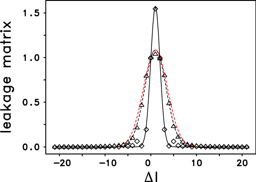
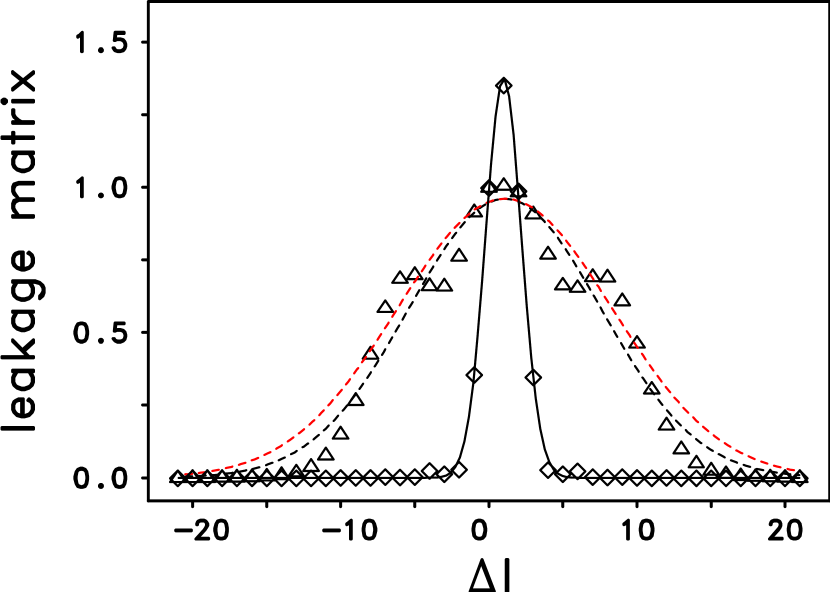
Figure 3: Dependence of $m$-averaged leakage matrix for a displacement component ratio of $c_{t}=1.0$ on the difference, $\Delta l=l^{\prime}-l$, between the degree $l^{\prime}$ of the spatial side-lobes and the degree $l$ of the target mode. The left panel is for $(n,l)=(0,400)$, while the right panel is for $(2,1000)$. The diamonds represent the original leakage matrix, while the triangles are for the leakage matrix which is corrected for the effect of the solar differential rotation. The full black lines are Gaussian fits to the uncorrected leakage matrices, and the dashed black lines are Gaussian fits to the corrected leakage matrices. The width of the corrected matrices increases considerably with increasing degree $l$. In each panel the dashed red line represents a Gaussian the full-width-at-half maximum (FWHM) of which is larger by a factor of 1.18 than the FWHM of the Gaussian shown by the black dashed line. These such distorted Gaussians are used in Section 5.2 to study the effect of changes in the FWHM of the leakage matrix upon the fitted mode parameters.

The Gaussian approximation, as defined in equation (22), to the $m$-averaged leakage matrix is implemented into the WMLTP method by means of the following approach. For given degree $l$ and radial order $n$, we first compute for a set of discrete values of the displacement component ratio (cf. Section 3.2.1), $c_{t}^{(n,l)}$,

$$c_{t,j}^{(n,l)}=j/10,\quad j=0,\ldots,10,$$ (23)

the $m$-averaged leakage matrix $C_{n;l,l^{\prime}}^{\,\mbox{\scriptsize(mavg)}}$ that has been corrected for the latitudinal differential rotation as described in Section 3.2.2. Next, we fit the Gaussian profile, as given in equation (22), to the resulting leakage matrices to get, for each of the values $c_{t,j}^{(n,l)}$, $j=0,\ldots,10$, the values $\alpha_{j}^{(n,l)}$ and $x_{m,j}^{(n,l)}$ of the fit parameters $\alpha^{(n,l)}$ and $x_{m}^{(n,l)}$, respectively, that determine the Gaussian profile, as defined in equation (22). Because the three parameters $\alpha^{(n,l)}$, $x_{m}^{(n,l)}$, and $c_{t}^{(n,l)}$ are not independent from one another, we follow Rhodes et al. (2001) and expand both $\alpha^{(n,l)}$ and $c_{t}^{(n,l)}$ in terms of $x_{m}^{(n,l)}$, viz.

$$\alpha^{(n,l)} = \bar{\alpha}_{0}^{(n,l)}+x_{m}^{(n,l)}\left(\bar{\alpha}_{1}^{(n,l)}+\bar{\alpha}_{2}^{(n,l)}x_{m}^{(n,l)}\right),$$ (24)

$$c_{t}^{(n,l)} = \bar{\beta}_{0}^{(n,l)}+x_{m}^{(n,l)}\left(\bar{\beta}_{1}^{(n,l)}+\bar{\beta}_{2}^{(n,l)}x_{m}^{(n,l)}\right),$$ (25)

where $\bar{\alpha}_{0}^{(n,l)}$, $\bar{\alpha}_{1}^{(n,l)}$, $\bar{\alpha}_{2}^{(n,l)}$, and $\bar{\beta}_{0}^{(n,l)}$, $\bar{\beta}_{1}^{(n,l)}$, $\bar{\beta}_{2}^{(n,l)}$ denote the respective expansion coefficients. We note that it would be mathematically equivalent to expand both $\alpha^{(n,l)}$ and $x_{m}^{(n,l)}$ in terms of $c_{t}^{(n,l)}$. In the final step of our approach we fit the expansion (24) to the knots $\left(\alpha_{j}^{(n,l)},x_{m,j}^{(n,l)}\right)$, $j=0,\ldots,10$, and the expansion (25) to the knots $\left(c_{t,j}^{(n,l)},x_{m,j}^{(n,l)}\right)$, $j=0,\ldots,10$, to get the set of expansion coefficients $\bar{\alpha}_{0}^{(n,l)}$, $\bar{\alpha}_{1}^{(n,l)}$, $\bar{\alpha}_{2}^{(n,l)}$, and $\bar{\beta}_{0}^{(n,l)}$, $\bar{\beta}_{1}^{(n,l)}$, $\bar{\beta}_{2}^{(n,l)}$. Typical fits of both $\alpha^{(n,l)}$ and $c_{t}^{(n,l)}$ versus $x_{m}^{(n,l)}$ are shown here in Figure 4 for the modes $(n,l)=(11,10)$, $(0,400)$, and $(2,1000)$, respectively. The fits clearly demonstrate that the expansions given in equations (24) and (25), respectively, are reasonable approximations to the variation of both $\alpha^{(n,l)}$ and $c_{t}^{(n,l)}$ with respect to $x_{m}^{(n,l)}$. Moreover, from the left panel in Figure 4 it becomes evident that $\alpha^{(n,l)}$ decreases with increasing degree $l$. Hence, according to equation (22) the width of the $m$-averaged leakage matrix increases with increasing degree $l$.

Once the set of expansion coefficients $\bar{\alpha}_{0}^{(n,l)}$, $\bar{\alpha}_{1}^{(n,l)}$, $\bar{\alpha}_{2}^{(n,l)}$, and $\bar{\beta}_{0}^{(n,l)}$, $\bar{\beta}_{1}^{(n,l)}$, $\bar{\beta}_{2}^{(n,l)}$ has been computed for the mode $(n,l)$, the corresponding $m$-averaged leakage matrix $\Lambda_{n,l}$, as given in equation (22), can easily be determined by performing the following steps. First, we calculate the value of $c_{t}^{(n,l)}$ from equation (9). Second, using this value of $c_{t}^{(n,l)}$ we solve equation (25) for $x_{m}^{(n,l)}$. Finally, we insert this value of $x_{m}^{(n,l)}$ into equation (24) to get the value of $\alpha^{(n,l)}$.

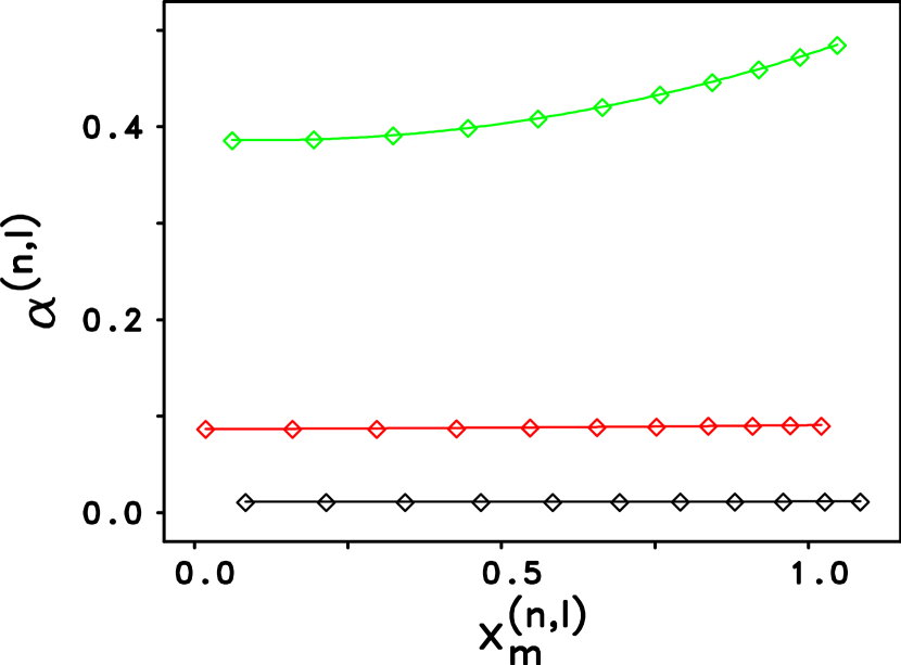
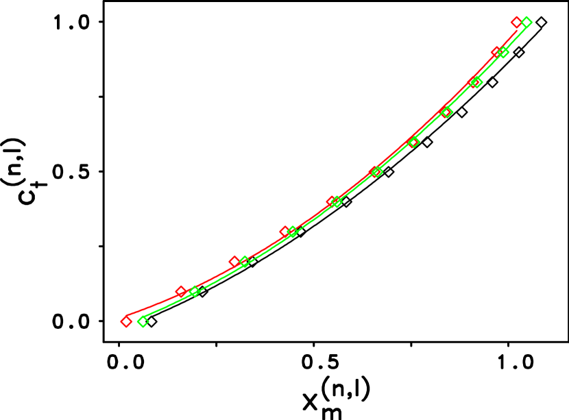
Figure 4: (left) Dependence of the parameter $\alpha^{(n,l)}$, which according to equation (22) is related to the width of the leakage matrix, on the offset, $x_{m}^{(n,l)}$, of the leakage matrix due to the horizontal component of the modal velocity eigenfunction for $(n,l)=(11,10)$ (green), $(0,400)$ (red), and $(2,1000)$ (black). The diamonds are for fits to a numerical representation of these leakage matrices that were corrected for the solar latitudinal differential rotation. The solid lines are for the parameterization as given in equation (24). We particularly note that for high degree values the parameter $\alpha^{(n,l)}$ is nearly independent of the value of $x_{m}^{(n,l)}$. (right) Same as left panel, but for the solar velocity eigenfunction component ratio, $c_{t}^{(n,l)}$. In this panel the solid lines are for the parameterization given in equation (25).

4.2 Theoretical fitting profile

In the WMLTP method the following fitting profile is used to represent an oscillation peak of given degree $l$ and radial order $n$:

$$M_{n,l}(\nu,\mbox{\boldmath$p$})=\mathcal{M}_{n,l}(\nu,\mbox{\boldmath$p$})\otimes\mathcal{W}(\nu).$$ (26)

Here, $\nu$ is frequency, $\mathcal{W}(\nu)$ is the Fourier spectrum of the temporal window function of the observational time series, “$\otimes$” denotes the convolution operator, and $\mathcal{M}_{n,l}(\nu,\mbox{\boldmath$p$})$ is defined by

$$\mathcal{M}_{n,l}(\nu,\mbox{\boldmath$p$}) =\underbrace{\sum_{\Delta l=-M}^{M}\Psi(A_{n,l},B_{n,l},x_{\Delta l})\,\Theta(\Delta l)\,\Lambda_{n,l}(\Delta l,\alpha^{(n,l)},x_{m}^{(n,l)})}_{\mbox{targeted peak and $l$-leaks}}+\underbrace{\sum_{i=1}^{N}\Psi(A_{i},B_{i},x_{i}),}_{\mbox{$n$-leaks}}$$ (27)

$$+\underbrace{a+b\,\nu+c\,\nu^{2}}_{\mbox{background}},$$

where

$$\Psi(A,B,x)=A\,\frac{(1+Bx)^{2}+B^{2}}{1+x^{2}},$$ (28)

$$\Theta(\Delta l)=1+\sum_{\mu=1}^{\mu_{\rm max}}\frac{1}{\mu!}\frac{1}{A}\frac{\partial^{\mu}A}{\partial l^{\mu}}\left(\Delta l\right)^{\mu},$$ (29)

$$x_{\Delta l}=\frac{2\left[\nu-\left(\nu_{n,l}+\displaystyle\sum_{\mu=1}^{\mu_{\rm max}}\displaystyle\frac{1}{\mu!}\frac{\partial^{\mu}\nu}{\partial l^{\mu}}\left(\Delta l\right)^{\mu}\right)\right]}{w_{n,l}\left(1+\displaystyle\sum_{\mu=1}^{\mu_{\rm max}}\displaystyle\frac{1}{\mu!}\frac{1}{w}\frac{\partial^{\mu}w}{\partial l^{\mu}}\left(\Delta l\right)^{\mu}\right)},$$ (30)

$$x_{i}=\frac{2\,(\nu-\nu_{i})}{w_{i}}.$$ (31)

Here, $\Psi$ is the asymmetric profile of Nigam & Kosovichev (1998), $\Theta$ is an empirical adjustment to the amplitudes of the $l$-leaks, $\Lambda_{n,l}$ is an approximation to the $m$-averaged leakage matrix that is described in Section 4.1, $2M$ is the number of the $l$-leaks, $N$ is the number of the $n$-leaks, $A_{i}$, $B_{i}$, $\nu_{i}$, and $w_{i}$ are, respectively, the amplitude, the line asymmetry parameter, the frequency, and width of the $i$-th $n$-leak, $i=1,\ldots,N$, and $a$, $b$, $c$ are parameters describing the background noise. We note that in equation (27) it has been presumed that each of the $2M+1$ modal peaks can be characterized by the same line asymmetry parameter $B_{n,l}$.

The total number of $l$-leaks, $2M$, included in the model profile, as given in equation (27), depends on the width of the leakage matrix, $\Lambda_{n,l}$, and is typically in the range from 10 to 60. As we have noted in Section 4.1, particularly for higher degrees, $l$, the leakage matrices are rather wide which is mainly due to the distortion of the oscillation eigenfunctions caused by the latitudinal differential rotation. Therefore, in equations (29) and (30) Taylor series expansions of fairly high order have to be employed to adequately describe the variation of amplitude, frequency, and linewidth with degree $l$. In the current version of the WMLTP code $\mu_{\rm max}=8$ is used. For the determination of the total number of $n$-leaks, $N$, to be included in the model profile given by equation (27), we refer the reader to Section 4.4. In our applications we found that $N$ can vary from 0 up to about 23, depending on both degree $l$ and radial order $n$.

In the fitting profile defined in equations (26) through (31) a total of $4N+8$ fitting parameters are involved, viz. the mode amplitude $A_{n,l}$, the mode frequency $\nu_{n,l}$, the mode linewidth $w_{n,l}$, the background noise parameters $a$, $b$, $c$, the line asymmetry parameter $B_{n,l}$, the offset, $x_{m}^{(n,l)}$, of the $m$-averaged leakage matrix due to the horizontal component of the modal velocity eigenfunction of the Sun (cf. Sect. 4.1), and the parameters $A_{i}$, $\nu_{i}$, $w_{i}$, $B_{i}$, $i=1,\ldots,N$, representing, respectively, amplitude, frequency, linewidth, and line asymmetry of the $N$ $n$-leaks. These fitting parameters can be lumped together in the fitting vector

$$\mbox{\boldmath$p$}=\left(A_{n,l},\nu_{n,l},w_{n,l},B_{n,l},a,b,c,x_{m}^{(n,l)},A_{1},\nu_{1},w_{1},B_{1},\ldots,A_{N},\nu_{N},w_{N},B_{N}\right)^{\mbox{\footnotesize T}}.$$ (32)

We did not include in this fitting vector $p$ the parameter $\alpha^{(n,l)}$ because it depends on $x_{m}^{(n,l)}$ by virtue of equation (24). We also did not include the Taylor series expansion coefficients

$$\frac{1}{A}\frac{\partial^{\mu}A}{\partial l^{\mu}},\,\,\,\frac{\partial^{\mu}\nu}{\partial l^{\mu}},\,\,\,\frac{1}{w}\frac{\partial^{\mu}w}{\partial l^{\mu}},\quad\mu=1,\ldots,\mu_{\rm max},$$ (33)

for the amplitude, frequency, and linewidth, respectively. Rather, these coefficients are taken, for given degree $l$ and radial order $n$, from tables containing initial estimates or so-called seeds that are derived from previously computed modal parameters, and are improved upon in a fixed-point iteration similar to that described in Rhodes et al. (2001). As a result, the compilation of such seed tables is an important pre-processing step for the use of the WMLTP method.

In order to investigate the performance of our implemented fixed-point iteration we have done the following analysis in which we have restricted ourselves to the investigation of the frequency, $\nu$, and the derivative thereof with respect to degree, $\Delta\nu/\Delta l$. For convenience, we did not consider either the linewidth or the amplitude and the derivatives thereof with respect to degree. In the first step of this analysis we used our seed table for the epoch of 2010 which provided both the seed frequencies, $\nu_{n,l}^{\rm(seed,1)}$, and the derivative thereof with respect to degree, $\left(\Delta\nu/\Delta l\right)_{n,l}^{\rm(seed,1)}$, to fit the $m$-averaged spectral set $\cal{S}$2001_90. From this fitting run we obtained the frequencies, $\nu_{n,l}^{\rm(fit,1)}$. We chose the $m$-averaged spectral set $\cal{S}$2001_90 for this test because the $\cal{R}$2001_90 observing run corresponded to the maximum phase of Solar Cycle 23. Therefore, due to the well-known shifts in the $f$- and $p$-mode frequencies that accompany changes in solar activity, the fitted frequencies, and the frequency derivatives, that would result from the fitting of these power spectra, would be expected to exhibit the largest possible differences from the frequencies and derivatives in our 2010 seed table since the latter were generated from the $\cal{R}$2010_66 observing run when the mean level of solar activity was much lower.

Next, we fitted to the frequencies, $\nu_{n,l}^{\rm(fit,1)}$, on a ridge-by-ridge basis, a smooth function of degree, $P^{(n)}(l)$, to get new seeds $\nu_{n,l}^{\rm(seed,2)}$ and $\left(\Delta\nu/\Delta l\right)_{n,l}^{\rm(seed,2)}$, respectively, by setting

$$\nu_{n,l}^{\rm(seed,2)} =P^{(n)}(l),$$ (34)

$$\left(\frac{\Delta\nu}{\Delta l}\right)_{n,l}^{\rm(seed,2)} =\left.\frac{\partial P^{(n)}(l)}{\partial l}\right|_{l},$$ (35)

where the superscript “$(n)$” denotes the ridge of radial order $n$. For the details of the construction of the function, $P^{(n)}(l)$, we refer the reader to the end of Section 6.2. In the second step we used this new set of seeds to fit the $m$-averaged spectral set $\cal{S}$2001_90 once again to get the frequencies $\nu_{n,l}^{\rm(fit,2)}$, from which we generated yet another set of seeds $\nu_{n,l}^{\rm(seed,3)}$ and $\left(\Delta\nu/\Delta l\right)_{n,l}^{\rm(seed,3)}$, respectively, in the same manner as we have done in the previous step. These new seeds were then used to fit, in the third and final step, the $m$-averaged spectral set $\cal{S}$2001_90 a third time to get the fitted frequencies, $\nu_{n,l}^{\rm(fit,3)}$. For further explanation we have illustrated the sequence of individual steps performed in our analysis in Figure 5.

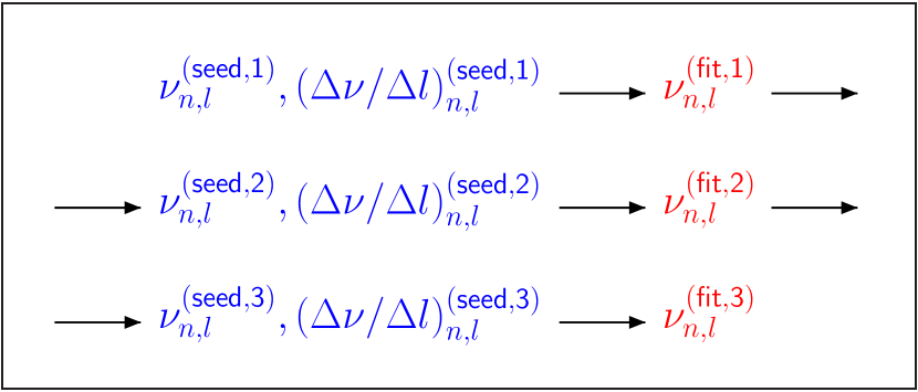
Figure 5: Flow chart of the individual steps performed in the fixed-point iteration for the construction of accurate seed tables using the example of the frequency, $\nu$. Similar flow charts apply to amplitude and linewidth, respectively.

The results of our analysis are summarized in Table 3. As can be seen from columns 4 and 5, the two-fold update of the seed table resulted in a significant reduction in both the average and the standard deviation of the differences of the seed values of $\Delta\nu/\Delta l$ as well as of the scaled differences of the fitted frequencies. As expected, the rather large changes in the scaled differences of the fitted frequencies that accompanied the first update of our 2010 seed table were reflective of the very large difference in the mean levels of activity between 2001 and 2010. The fact that we could obtain a self-consistent seed table for 2001 with only two iterations in spite of such a large difference in the level of activity in the two epochs justifies our approach of replacing the Taylor series expansions, as given in equation (33), with such self-consistent seed values.

4.3 Selection of fitting box widths

The width of the selected fitting box is crucial for the successful determination of the fitting vector $p$ defined in equation (32). We have found it useful to construct the fitting box for the mode $(n,l)$ as follows:

$$\nu_{n,l}^{\rm low}=\nu_{n,l}^{\rm seed}-\tau^{(n,l)}\,\frac{\Delta\nu_{n,l}}{\Delta n}\bigg{|}_{\rm left},\quad\nu_{n,l}^{\rm up}=\nu_{n,l}^{\rm seed}+\tau^{(n,l)}\,\frac{\Delta\nu_{n,l}}{\Delta n}\bigg{|}_{\rm right}.$$ (36)

Here, $\nu_{n,l}^{\rm seed}$ is the seed frequency of the targeted mode $(n,l)$, $\nu_{n,l}^{\rm low}$ and $\nu_{n,l}^{\rm up}$ are the lower and upper boundary, respectively, of the fitting box, $\Delta\nu_{n,l}/\Delta n|_{\rm left}$ and $\Delta\nu_{n,l}/\Delta n|_{\rm right}$ denote the variation of the mode frequency with respect to the radial order $n$ at the left (i.e., lower frequency) and right (i.e., higher frequency) side, respectively, and $\tau^{(n,l)}$ is given by

$$\tau^{(n,l)}=\left\{\begin{array}[]{l@{\quad}l}\tau_{1}^{(n)}&\mbox{for~{}~{}$l\leq l_{1}^{(n)}$,}\\[2.84526pt] \displaystyle\frac{\tau_{2}^{(n)}-\tau_{1}^{(n)}}{l_{2}^{(n)}-l_{1}^{(n)}}\,\left(l-l_{1}^{(n)}\right)+\tau_{1}^{(n)}&\mbox{for~{}~{}$l_{1}^{(n)}<l<l_{2}^{(n)},$}\\[13.37277pt] \tau_{2}^{(n)}&\mbox{for~{}~{}$l\geq l_{2}^{(n)}$,}\end{array}\right.$$ (37)

where $\tau_{1}^{(n)}$, $\tau_{2}^{(n)}$, $l_{1}^{(n)}$, and $l_{2}^{(n)}$ are predetermined parameters depending on the radial order $n$. The quantities $\Delta\nu_{n,l}/\Delta n|_{\rm left}$ and $\Delta\nu_{n,l}/\Delta n|_{\rm right}$ in equation (36) are approximated as follows:

$$\begin{array}[]{l@{\quad}l}\displaystyle\frac{\Delta\nu_{n,l}}{\Delta n}\bigg{|}_{\rm left}\approx\nu_{n,l}^{\rm seed}-\nu_{n-1,l}^{\rm seed},\quad\frac{\Delta\nu_{n,l}}{\Delta n}\bigg{|}_{\rm right}\approx\nu_{n+1,l}^{\rm seed}-\nu_{n,l}^{\rm seed}&\mbox{for~{}~{}$n>0$,}\\[14.22636pt] \displaystyle\frac{\Delta\nu_{n,l}}{\Delta n}\bigg{|}_{\rm left}=\frac{\Delta\nu_{n,l}}{\Delta n}\bigg{|}_{\rm right}\approx\nu_{n+1,l}^{\rm seed}-\nu_{n,l}^{\rm seed}&\mbox{for~{}~{}$n=0$,}\end{array}$$ (38)

where $\nu_{n,l}^{\rm seed}$, $\nu_{n-1,l}^{\rm seed}$, and $\nu_{n+1,l}^{\rm seed}$ are taken from a seed table. As to the choice of the parameters $\tau_{1}^{(n)}$, $\tau_{2}^{(n)}$, $l_{1}^{(n)}$, and $l_{2}^{(n)}$ in equation (37) it must be kept in mind that any selected fitting box must fulfill at least two requirements. First, the fitting box must be sufficiently wide so that both the mode profile and the background power are well sampled. This requirement becomes an issue if spectra are to be fitted that are derived from an observing run the duration of which is only a few days. In this case it can happen that the number of fit parameters included in the fitting vector $p$ exceeds the number of frequency bins constituting the fitting box. Second, the fitting box must not be unduly wide in order to save computing time which non-linearly increases with the number of frequency bins comprising the fitting box. In practice, we determine the parameters $\tau_{1}^{(n)}$, $\tau_{2}^{(n)}$, $l_{1}^{(n)}$, and $l_{2}^{(n)}$ for a given ridge of radial order, $n$, by a trial-and-error method and select those values of them which give rise to the least scatter of frequency along the ridge.

As can be seen from equations (36) and (37), aside from variations of both $\Delta\nu_{n,l}/\Delta n|_{\rm left}$ and $\Delta\nu_{n,l}/\Delta n|_{\rm right}$ with degree $l$, the width of the fitting box is constant for $l\leq l_{1}^{(n)}$ and $l\geq l_{2}^{(n)}$, and varies linearly with degree $l$ for $l_{1}^{(n)}<l<l_{2}^{(n)}$. We note here that in general $\Delta\nu_{n,l}/\Delta n|_{\rm left}\neq\Delta\nu_{n,l}/\Delta n|_{\rm right}$. Therefore, according to equation (36) the fitting box is generally not symmetric with respect to the seed frequency $\nu_{n,l}^{\rm seed}$.

For a selected set of radial orders, $n$, we show in Figure 6 the half of the width, $w_{b}$, of the respective fitting boxes measured in terms of the average, $\langle\Delta\nu/\Delta n\rangle$, of $\Delta\nu_{n,l}/\Delta n|_{\rm left}$ and $\Delta\nu_{n,l}/\Delta n|_{\rm right}$. For most of the cases shown the width of the fitting box increases with increasing degree, while for $n=6$ the width is practically constant, and for $n=8$ and $n=29$ the width decreases with degree. We also note that for the higher-order ridges the $n$-leaks $(n\pm 1,l)$ are included in the fitting box. For the $n=20$ ridge the fitting box is getting so wide that even the $n$-leaks $(n\pm 2,l)$ are encompassed. The choice of such wide fitting boxes is expressive of the fact that, in general, the scatter of the fitted mode parameters along a given ridge decreases with increasing width of the fitting boxes. Therefore, it would be desirable to fit all $n$-values simultaneously that are present in an $m$-averaged spectrum of given degree. However, such approach is not feasible on practical grounds.

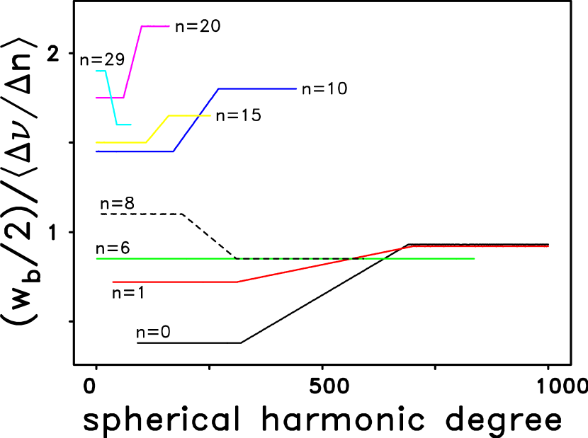
Figure 6: Half of the width, $w_{b}$, of the fitting box measured in terms of $\langle\Delta\nu/\Delta n\rangle$ versus degree for a selected set of radial orders, $n$. Here, $\langle\Delta\nu/\Delta n\rangle$ denotes the mean value of $\Delta\nu_{n,l}/\Delta n|_{\rm left}$ and $\Delta\nu_{n,l}/\Delta n|_{\rm right}$ with $\Delta\nu_{n,l}/\Delta n|_{\rm left}$ and $\Delta\nu_{n,l}/\Delta n|_{\rm right}$ being the variation of the target mode frequency with respect to the radial order, $n$, at the lower and the higher frequency side of the fitting box, respectively. For most cases shown the fitting box widens with increasing degree by only about 10 to 30 %, while it widens by about 150 % for the $n=0$ ridge. However, for the $n=8$ and $n=29$ ridge the width decreases with degree by about 23 % and 15 %, respectively. For the $n=6$ ridge the width is practically constant. For the $n=20$ ridge the $n$-leaks $(n\pm 1,l)$ and $(n\pm 2,l)$ are located within the fitting box for higher degrees.

4.4 Determination of the number of n-leaks to be included in the fitting model profile

The number of $n$-leaks, $N$, to be included in the fitting model profile defined by equations (26) through (31), cannot be determined from first principles. Therefore, a range $|l-l_{0}|\leq l_{\rm range}$, $|n-n_{0}|\leq n_{\rm range}$, of $l$ and $n$ values is chosen around the targeted mode $(n_{0},l_{0})$, and every mode $(n,l)$ within this range that (1) has a frequency within the frequency range of the fitting box (cf. Section 4.3), (2) differs from $(n_{0},l_{0})$, and (3) is not identical to any of the $l$-leaks, is included as an $n$-leak in equation (27). In the current version of the WMLTP code we are using $l_{\rm range}=4$, $n_{\rm range}=3$ for isolated modal peaks, $(n_{0},l_{0})$, and $l_{\rm range}=4$, $n_{\rm range}=2$ otherwise. Usually, many of the $n$-leaks determined in this manner turn out to be statistically insignificant for getting a reasonably good fit. Because generally the $n$-leaks included in the fitting profile strongly affect the fitted parameters of the targeted mode $(n_{0},l_{0})$, it is crucial to discard the statistically insignificant $n$-leaks while keeping the statistically significant ones. Therefore, the statistical significance of an $n$-leak is tested by virtue of the so-called R-test (Frieden, 1983). This test is skipped, however, for “true” $n$-leaks $(n_{0}\pm 1,l)$ and $(n_{0}\pm 2,l)$, respectively, with $(n_{0},l_{0})$ being the targeted mode. Because the R-test does not always work satisfactorily, we have additionally implemented into the WMLTP code heuristic criteria for discarding an $n$-leak. For example, an $n$-leak is discarded if its amplitude and/or width is outside a given range or if it overlaps too much with another $n$-leak or with the targeted peak itself. Overall, the determination of the number of $n$-leaks, $N$, is a rather time consuming undertaking which significantly increases the compute time of the WMLTP code.

4.5 Implementation of numerical scaling, adjustments, and options

The vector $p$ defined in equation (32) is determined by fitting, in the least-squares sense, the model profile given in equations (26) through (31) to the $m$-averaged spectrum of given degree $l$ in a fitting box (cf. Section 4.3) centered about the target peak of radial order $n$. The confidence interval on each fit parameter $p_{i}\in\mbox{\boldmath$p$}$ is calculated as described in Appendix A. In order to make the solution of this least-squares problem as robust as possible diverse provisions are made. First, all fit parameters are scaled such as to make their values on the order of unity. This scaling greatly improves the numerical stability of the solution of the least-squares problem. Second, the fit parameters representing the target peak (viz. $A_{n,l}$, $\nu_{n,l}$, $w_{n,l}$, $B_{n,l}$) as well as the fit parameters representing the $n$-leaks (viz. $A_{i}$, $\nu_{i}$, $w_{i}$, $B_{i}$, $i=1,\ldots,N$) are subject to bounds, i.e., they are constrained to lie within prescribed intervals. This is important in order to avoid unphysical values of any of these fit parameters, for example, negative amplitudes, frequencies too much off from their seed values, linewidths much smaller than the spectral resolution, or linewidths on the order of the width of the fitting box. Also, the magnitude of the line asymmetry parameter of both the target peak and the $n$-leak peaks is constrained to values less than or equal to 0.3. Third, the fitting vector $p$ is determined in several passes. In Table 4 it is shown which parameters are fitted in the individual passes. Any parameter not listed in a given pass as a fitted parameter in Table 4, but which is included in the fitting vector $p$, is kept fixed either to its seed value or else to its value obtained in a previous pass. We note that the permutations given in Table 4 were chosen on purely heuristic grounds and are, therefore, somewhat arbitrary. Fourth, a flag can be set in the WMLTP code which enforces the use of the symmetric Lorentzian profile. This is accomplished by setting $B=0$ in equation (28). Otherwise, the full asymmetric profile is used, in which case the asymmetry parameter, $B$, in equation (28) is employed as a fitting parameter in the least-squares problem.

For the solution of the nonlinear constrained least-squares problem which results for the determination of the fitting vector $p$ we use the FORTRAN code NLPQL which is a special implementation of a so-called sequential quadratic programming method, and which is generally designed for solving constrained non-linear optimization problems (Schittkowski, 1986). Sequential quadratic programming is one of the most robust algorithms for the solution of non-linear continuous optimization problems. The method is based on solving a series of sub-problems designed to minimize a quadratic approximation to the Lagrangian function subject to a linearization of the constraints.

In the case of either high frequencies and/or high degrees when the individual modal peaks can no longer be resolved but rather blend together to form ridges of power in the $m$-averaged spectra, the determination of the fitting vector $p$ given in equation (32) becomes an ill-defined least-squares problem. This is because in this case any change of the parameter $x_{m}^{(n,l)}$ does not result in a significant change of the fitting profile defined by equations (26) through (31) because $\alpha^{(n,l)}$, which is related to the width of the leakage matrix, turns out to be practically independent of $x_{m}^{(n,l)}$, as is demonstrated here in the left panel of Figure 4. As a result, $x_{m}^{(n,l)}$ can no longer be used as a fit parameter but rather must be kept fixed to its seed value.

To make the WMLTP method more flexible in practical applications we have implemented the following features into the code. First, if frequency splitting coefficients are available for a mode $(n,l)$, the $m$-averaged spectrum can be calculated from the respective zonal, sectoral, and tesseral spectra in a weighted or unweighted fashion within the fitting box of that mode making superfluous the calculation of the $m$-averaged spectrum in the pre-processing step as described in Section 2.2. In other words, this option makes it possible to either use splitting coefficients or else an $m$-averaged spectrum as input to the WMLTP code. This feature is particularly useful if non-$n$-averaged splitting coefficients are available. Second, for a mode $(n,l)$ the expansion coefficients which are required to calculate the corresponding $m$-averaged leakage matrix parameters $\alpha^{(n,l)}$ and $x_{m}^{(n,l)}$ via equations (24) and (25), can either be read from a file generated in a previous calculation or else can be calculated as part of the fitting procedure itself. This way a considerable amount of compute time can be saved. Third, if the spectral peak of a mode $(n,l)$ is well separated from the $l$- and $n$-leak peaks, the offset parameter of the leakage matrix, $x_{m}^{(n,l)}$, can be invoked as a fit parameter. By then converting the fitted values of $x_{m}^{(n,l)}$ into values of $c_{t}^{(n,l)}$ by means of equation (25), Rhodes et al. (2001) were able to demonstrate, using a previous version of the WMLTP code, that the such measured values of $c_{t}^{(n,l)}$ match theoretical predictions. Broadly speaking, such approach is possible for modes with $w_{n,l}\lesssim 0.8\,(\Delta\nu/\Delta l)_{n,l}$, where $w_{n,l}$ is the mode linewidth and $(\Delta\nu/\Delta l)_{n,l}$ is an approximation to the derivative of the mode frequency with respect to degree.

4.6 Enforcement of symmetrical line profile for the fitting of pseudo-modes

We initially employed the asymmetrical profile for all of the cases along each ridge. However, for frequencies $\nu\gtrsim 5000\,\,\mu$Hz we found unexpected excursions in the line asymmetry parameter, $B$, an example of which is shown here for the $n=6$ ridge in the left panel of Figure 7. Because such behavior of the line asymmetry parameter, $B$, is hard to explain on physical grounds, we rather presume that the asymmetrical profile becomes invalid for modes with frequencies close to or greater than the acoustic cut-off frequency. This presumption is substantiated by the fact that for those frequencies the assumptions made by Nigam & Kosovichev (1998) in the derivation of their asymmetrical profile are not fulfilled. This is because the high-frequency peaks are not normal modes but rather so-called pseudo-modes caused by interference between the waves coming directly from the excitation source and waves refracted in the interior. Hence, the pseudo-modes are not oscillations that are trapped in the solar interior (Nigam et al., 1998; Nigam & Kosovichev, 1998). Moreover, the pseudo-mode spectral peaks are essentially symmetric. Asymptotically, at high frequencies, their profile is described by a $\sin^{2}$ function. Unfortunately, there is no simple fitting formula describing both normal modes and pseudo-modes. Because we need to leave the rather complicated issue of the proper profile to be employed as a subject of further investigation, we rather decided to resort to the workaround to simply force the fitting code to switch from the asymmetrical to the symmetrical profile at a prescribed frequency, $\nu_{s}$, along a given ridge. This switchover frequency is chosen to coincide with the first zero-crossing of the line asymmetry parameter, $B$, that occurs for frequencies $\nu\gtrsim 4600\,\,\mu$Hz along a given ridge. For example, for the $n=6$ ridge the switchover frequency is $\nu_{s}=4815\,\,\mu$Hz, as is shown here in the right panel of Figure 7. Expectedly, a sharp kink is introduced in the run of $B$ at the switchover frequency. Of course, a more physically motivated fitting profile would give rise to a gradual transition between the asymmetrical and the symmetrical profile. We point out that the switchover frequency $\nu_{s}$ depends not only on the radial order $n$ but also on the epoch of the observation, because the mode parameters are affected by the mean level of solar activity during each observing run.

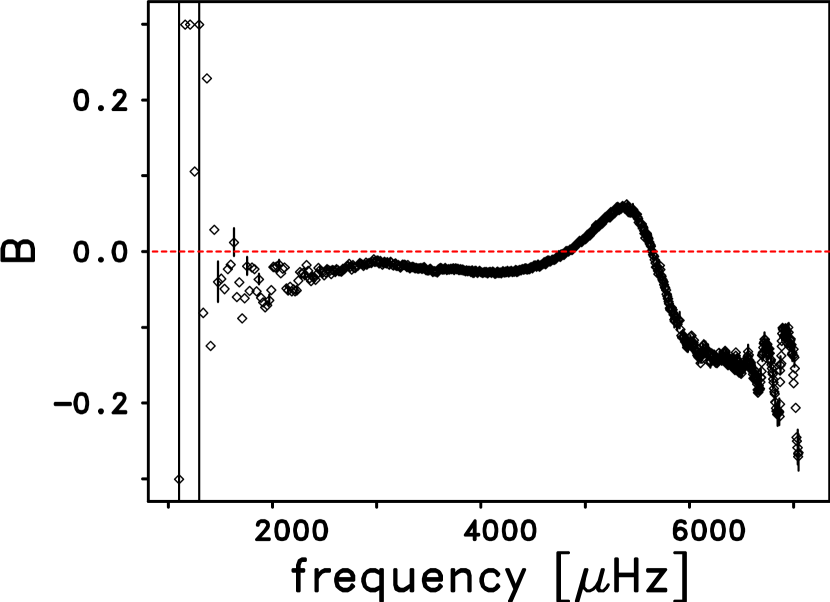
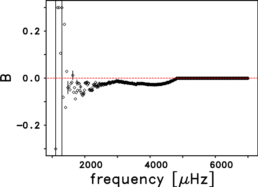
Figure 7: (left) Line asymmetry parameter $B$ versus frequency for the $n=6$ ridge computed from the $m$-averaged spectral set $\cal{S}$2010_66a. The error bars shown for selected values of frequency are for $1\,\sigma$ errors. Because the excursions of $B$ to both positive and negative values for $\nu>5000\,\,\mu$Hz are hard to explain on physical grounds, we switched over to a symmetric Lorentzian profile for the high-frequency portion of each ridge. (right) Same as left panel, except that the symmetrical profile was used for frequencies $\nu>4815\,\,\mu$Hz for this ridge. In both panels the red dashed line is for $B=0$.

At a glance, the tiny error bars as shown in the left panel of Figure 7 seem to indicate that the excursions of the line asymmetry parameter, $B$, to both positive and negative values for frequencies $\nu\gtrsim 5000\,\,\mu$Hz are a statistically significant effect. This is not the case, however. Rather this “significant” asymmetry in the fitted line profiles is a further argument that the asymmetric profile of Nigam & Kosovichev (1998) is invalid for the fitting of pseudo-modes. Namely, if it were valid, the resulting line asymmetry should be statistically compatible with $B=0$ for frequencies $\nu\gtrsim 5000\,\,\mu$Hz because it is known that the pseudo-mode peaks are essentially symmetric.

The use of the symmetrical profile for frequencies above the switchover frequency, $\nu_{s}$, along a given ridge not only resolves the issue of the unexpected excursions in the line asymmetry parameter, $B$, but also results in a substantial reduction in the frequency scatter observed in the high-frequency portion of each ridge. For the study of the variation in the frequency scatter along a given ridge we found it useful to evaluate the point-to-point scatter, $\varSigma$, as defined by equation (B1), not for the frequency $\nu$ itself but rather for the numerical derivative of the frequency with respect to degree, $\Delta\nu/\Delta l$. An example of the reduction in the scatter of $\Delta\nu/\Delta l$ for frequencies above the switchover frequency is shown here for the $n=4$ ridge in Figure 8. For this ridge the switchover frequency is $\nu_{s}=4700\,\,\mu$Hz. In the left panel of Figure 8 the asymmetrical profile has been used for all of the cases along this ridge, while in the right panel the asymmetrical profile has been replaced with the symmetrical profile for frequencies $\nu>\nu_{s}$, i.e., for degrees $l\geq 562$. In order to evaluate the obvious reduction in the frequency scatter quantitatively, we computed $\varSigma$ for the high-frequency portion of the $n=4$ ridge by setting $l_{\rm min}=562$, $l_{\rm max}=1000$, and $\upsilon\equiv\Delta\nu/\Delta l$ in equation (B1). When we did so, we found after eliminating some obvious gross outliers that $\varSigma=0.639$ for the asymmetrical profile, but only $0.214$ for the symmetrical profile. Hence, by simply changing over from the asymmetrical to the symmetrical profile at $\nu=\nu_{s}$, we were able to reduce the scatter in $\Delta\nu/\Delta l$ by a factor of about 3. We also saw similar reductions in the scatter in the high-frequency cases of $\Delta\nu/\Delta l$ when we employed the symmetrical profile in place of the asymmetrical profile for the high-frequency portions of the $f$-mode and the other $p$-mode ridges.

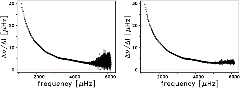
Figure 8: Frequency dependence of the numerical derivative of the frequency with respect to degree, $\Delta\nu/\Delta l$ (in $\mu$Hz), for the $n=4$ ridge. In the left panel the asymmetrical profile has been used for fitting all of the cases for this ridge, while in the right panel the asymmetrical profile has been replaced with the symmetrical profile for frequencies $\nu>4700\,\,\mu$Hz. Both sets of fits were computed from the $m$-averaged spectral set $\cal{S}$2010_66a. The error bars that are shown for selected cases are $1\,\sigma$ errors. The dashed red line is for $\Delta\nu/\Delta l=0$.

4.7 Determination of the background portion of the theoretical model profile

A power spectrum computed from a time series of Dopplergrams of length $T$ has a spectral resolution of $\Delta\nu=1/T$. If the Dopplergrams are observed at a cadence of $\Delta t$ the spectrum covers a frequency range from zero up to the Nyquist frequency $\nu_{\rm Ny}=1/(2\Delta t)$, which is $8333\,\,\mu$Hz for the MDI instrument, as we have already pointed out in Section 2.1. On the other hand, the maximum width, $W_{\rm max}$, of the fitting boxes used for fitting the modal peaks in the set of spectra obtained from an observing run is on the order of a few hundred $\mu$Hz at most. Hence, for $T$ being greater than a day or so, we have

$$\Delta\nu\ll W_{\rm max}\ll\nu_{\rm Ny}.$$ (39)

The inequality $W_{\rm max}\ll\nu_{\rm Ny}$ in the above equation (39) implies that we can safely approximate the background noise present in the measured power spectra as a quadratic function of frequency within a selected fitting box. We note, however, that generally a linear background model, i.e., $c=0$ in equation (27), is an adequate choice. We also note that the background portion of the theoretical model profile, as given in equations (26) through (31), is not a reliable estimate of the actual frequency variation of the background noise within the selected fitting box around the targeted peak. This is evident from the fact that the fit parameters $a$, $b$, and $c$ in equation (27), which describe the background portion of the model profile, can change significantly from one degree to the next along a given ridge. This scatter in the background portion of the model profile is most likely an artificial effect, and unfortunately translates into a similar scatter in other fitting parameters included in the model profile, such as frequency and linewidth, for example. To mitigate this scatter, we devised the following heuristic approach. First, we fit a straight line to the spectral power in the troughs of the spectrum in a frequency range that is twice as large than the fitting box centered around the targeted peak to estimate the slope of the background noise. This is demonstrated here in Figure 9 where we show, for the modes $(n,l)=(24,8)$, and $(24,56)$, respectively, the measured power spectrum in black with the such fitted straight line overlaid in red. While the troughs in a spectrum are not indicative of the background noise, but rather correspond to the intersection of the wings of the peaks, we believe that they are indicative of the slope of the background. Second, if $b_{\rm e}$ denotes the slope of the such determined straight line and $\Delta b_{\rm e}$ the uncertainty thereof, we constrain the slope $b$ of the background term in equation (27) by

$$b_{\rm e}-3\,\Delta b_{\rm e}\leq b\leq b_{\rm e}+3\,\Delta b_{\rm e},$$ (40)

where the term $3\,\Delta b_{\rm e}$ allows for uncertainties in the value of $b_{\rm e}$. Third, we constrain the background term in equation (27) by

$$a+b\,\nu+c\,\nu^{2}\geq 0\quad\mbox{for all frequencies $\nu$ within the fitting box},$$ (41)

just to ensure that the estimated background noise is positive throughout the entire fitting box.

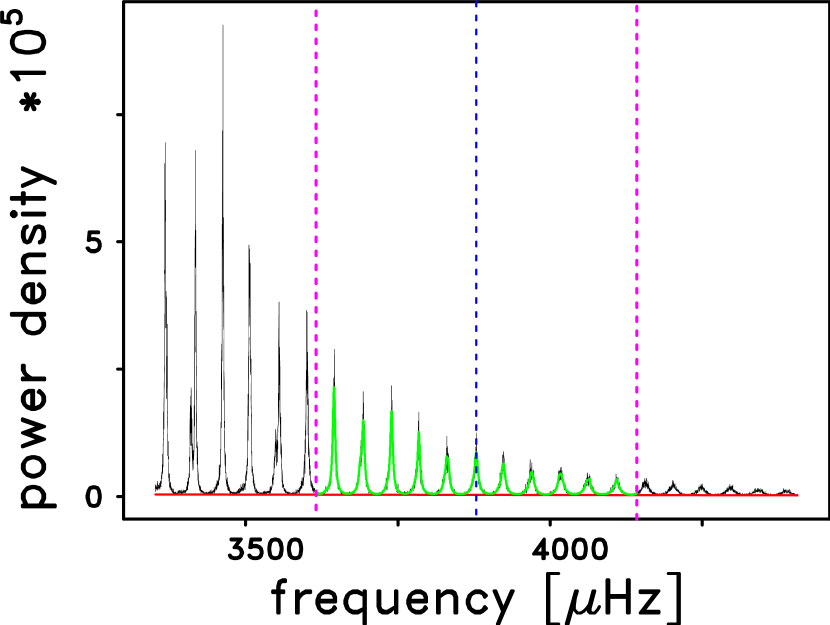
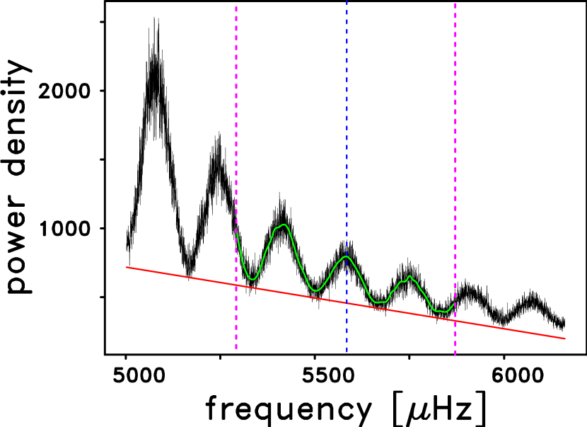
Figure 9: (left) Straight line fit to the spectral power density in the troughs of the spectrum of the $(n,l)=(24,8)$ mode, using the example of the $m$-averaged spectral set $\cal{S}$2010_66a. The spectral power density is shown in black, while the fitted line is shown in red. The slope of this fitted line is used as an estimate of the slope, $b$, of the background portion of the theoretical model profile given in equations (26) through (31), when this profile is fitted to the spectrum in the fitting box indicated by the vertical dashed lines in magenta. The fitted profile is shown as the green line, and the vertical blue dashed line is for the resulting fitted frequency. (right) Same as left panel, except that it is for the $(24,56)$ mode.

5 Sensitivity of Method 2 in terms of the m-averaging procedure and the effective leakage matrix

5.1 Sensitivity of Method 2 to details of the m-averaging procedure

In order to study the sensitivity of Method 2 to the details of the $m$-averaging procedure, as described in Section 2.2, we first used the Method 2 code to fit the four different sets of $m$-averaged power spectra $\cal{S}$2010_66a through $\cal{S}$2010_66d (cf. Table 2). From these fits we obtained four tables of fitted $f$- and $p$-mode parameters: frequencies, linewidths, amplitudes, line asymmetries, and their associated uncertainties. From these four tables of fitted parameters, we collected the frequencies and their uncertainties into four frequency tables, $\cal{F}$2010_66a through $\cal{F}$2010_66d, which we then inter-compared on a mode-by-mode basis. As one example of these four frequency tables, our table $\cal{F}$2010_66a covered the degree range of 0 to 1000, the radial order range of 0 to 29, and the frequency range of 965 to $7000\,\,\mu$Hz. Within these ranges of $l$, $n$, and $\nu$ we were able to obtain a total of 12,359 sets of converged frequencies and frequency uncertainties.

We note that we have limited our sensitivity study to the investigation of the impact of changes in the $m$-averaged spectra upon the fitted frequencies because the estimates of the mode frequencies are an essential part of any structural inversion.

5.1.1 The influence of the weighting of the un-averaged spectra

In order to study the possible influence upon the fitted frequencies of the weighting of the $2l+1$ un-averaged spectra at each degree in the computation of the $m$-averaged power spectra, as described in Section 2.2, we aligned our frequency tables $\cal{F}$2010_66a and $\cal{F}$2010_66b on a mode-by-mode basis, and we then subtracted the frequency of each mode in $\cal{F}$2010_66a from the corresponding frequency in $\cal{F}$2010_66b. The raw frequency differences that resulted, are shown in the two upper panels of Figure 10, where they are plotted, in the sense of “weighted” minus “unweighted”, as functions of both frequency and degree. Inspection of these two panels illustrates that the largest frequency differences corresponded primarily to the high-frequency portions of the ridges for degrees less than 350.

This concentration of the largest raw frequency differences at the higher frequencies is illustrated numerically in section C1 of Table 5, where we show in row 1 that the average magnitude of the differences for the frequency range $\nu<7000\,\,\mu$Hz is six times larger than the average magnitude of the cases for which $\nu<4500\,\,\mu$Hz. On the other hand, when we normalized these raw frequency differences by dividing each of them by its formal error, as is shown in the lower left panel of Figure 10, we found that only 4.6 % of them were statistically significant. This is also demonstrated in row 2 of Table 5, where we show that the average magnitude of the normalized frequency differences was about $1\,\sigma$ for both frequency ranges $\nu<7000\,\,\mu$Hz and $\nu<4500\,\,\mu$Hz, respectively.

Because most structural inversions have been limited to frequencies that have been less than $4500\,\,\mu$Hz, we also wanted to study the radial distribution of the normalized frequency differences for the cases that were below this limit. We found that 94.5 % of the cases that remained in this restricted frequency range were within the range of $\pm 3\,\sigma$. Furthermore, when we plotted the remaining normalized frequency differences as a function of the fractional inner turning-point radius of the corresponding modes, as shown in the lower-right panel of  Figure 10, we found that the majority of the cases that were the most significant were concentrated in the solar convection zone. In fact, very few of the normalized frequency differences exceeded $\pm 3\,\sigma$ inward of the base of the convection zone. Overall, Figure 10 indicates that the weighting of the un-averaged power spectra in the computation of the $m$-averaged power spectra had a very modest effect upon the fitted frequencies.

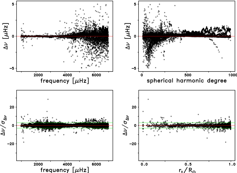
Figure 10: (upper-left) Frequency dependence of the frequency differences, $\Delta\nu$, which resulted from frequency tables $\cal{F}$2010_66a and $\cal{F}$2010_66b, in the sense of “weighted” minus “unweighted”. In each case, the same set of corrected, $n$-averaged frequency splitting coefficients has been used for the collapsing of the spectra. (upper-right) Degree dependence of the set of frequency differences, $\Delta\nu$, shown in the upper-left panel. (lower-left) Frequency dependence of the normalized frequency differences, $\Delta\nu/\sigma_{\Delta\nu}$. The normalization was carried out by dividing the raw frequency differences, $\Delta\nu$, as shown in the upper-left panel, by the formal error, $\sigma_{\Delta\nu}$, of each difference. (lower-right) Dependence of the low-frequency subset of the normalized frequency differences upon the fractional inner turning-point radii, $r_{\rm t}/R_{\odot}$, of those modes. Here, $R_{\odot}$ is the radius of the Sun. Only mode frequencies less than $4500\,\,\mu$Hz were included in this panel. In all four panels the red dashed line is for a frequency difference of zero. In the two panels in the lower row the green dashed lines show the $\pm 3\,\sigma$ values.

5.1.2 Influence of correction of frequency-splitting coefficients

In contrast to the situation that we just described in Section 5.1.1 for the construction of the $m$-averaged power spectra using both unweighted and weighted tesseral and sectoral power spectra, the correction of the un-corrected, non-$n$-averaged frequency splitting coefficients for the distortions introduced by the latitudinal differential rotation resulted in highly significant frequency differences for those cases that are used in structural inversions, as we have demonstrated in Figure 11. In the upper-left panel of this figure, we show the frequency dependence of the un-normalized frequency differences in the sense of “corrected” minus “un-corrected” that resulted when we subtracted the frequencies in table $\cal{F}$2010_66c from those in table $\cal{F}$2010_66d. In contrast to the upper-left panel of Figure 10, the majority of these frequency differences for the modes having $\nu<4500\,\,\mu$Hz were negative and the majority of the high-frequency differences were positive. In another contrast with the upper-left panel of Figure 10, there is a strong frequency dependence of the high-frequency differences shown in the upper-left panel of Figure 11. In a third contrast with the situation shown in Figure 10, the upper-right panel of Figure 11 shows that the positive frequency differences were not restricted to the lower-degree modes alone, but instead were present for all modes having degrees greater than 200. The negative frequency differences that are shown for $2500<\nu<4500\,\,\mu$Hz in the upper-left panel of Figure 11 corresponded to the $n=0$ through $n=3$ ridges. These negative differences indicate that the frequencies that were computed from the $m$-averaged power spectra that were computed using the corrected splitting coefficients were systematically smaller than were the frequencies for the same ridges that were fit to the averaged spectra that were generated using the un-corrected splitting coefficients. These systematic frequency differences resulted from the fact that the corrected splitting coefficients in this frequency range were generally smaller than their un-corrected counterparts.

When we normalized these raw frequency differences by dividing each of them by the formal uncertainty of the difference, we found that the most significant normalized differences corresponded to modes which have frequencies between 1800 and $4500\,\,\mu$Hz, as is shown here in the lower-left panel of Figure 11. In particular, the normalized frequency differences were highly significant for the $n=0$ through $n=2$ ridges. In the contrast to the situation for the raw frequency differences that are shown in the upper-left panel of this figure, the normalized frequency differences of the high-frequency modes were mainly less than $\pm 3\,\sigma$. When we restricted these normalized frequency differences to those having frequencies less than $4500\,\,\mu$Hz and plotted the remaining cases as a function of the fractional inner turning-point radius of the modes, as shown in the lower-right panel of Figure 11, we found that the cases with the highly-significant negative ratios were all concentrated in the shallow subphotospheric layers.

The statistics of both the raw and normalized frequency differences are listed in section C2 (i.e., rows 3 and 4) of Table 5. Here, we show in row 4 that the average magnitude of the normalized frequency differences for the frequency range $\nu<7000\,\,\mu$Hz was equal to $4.9\,\sigma$, while the average magnitude of the normalized frequency differences for the cases for which $\nu<4500\,\,\mu$Hz was equal to $7.8\,\sigma$. Furthermore, this average of $7.8\,\sigma$ is over 79 times its standard error away from zero. Clearly, the correction of the frequency-splitting coefficients that are used in the generation of $m$-averaged power spectra is an essential step.

A previous comparison of the sets of frequencies computed using both raw and corrected, $n$-averaged splitting coefficients had shown small enough frequency differences that led us to believe that the rather time-consuming correction of more than 12,000 raw, non-$n$-averaged splitting coefficients would not be necessary. However, in response to the suggestion of the anonymous referee that we investigate the effects of making such corrections, we found significant differences in the sets of frequencies computed using the raw and corrected, non-$n$-averaged splitting coefficients, as is demonstrated here in the fourth row of Table 5, (i.e., the second row of Section C2).

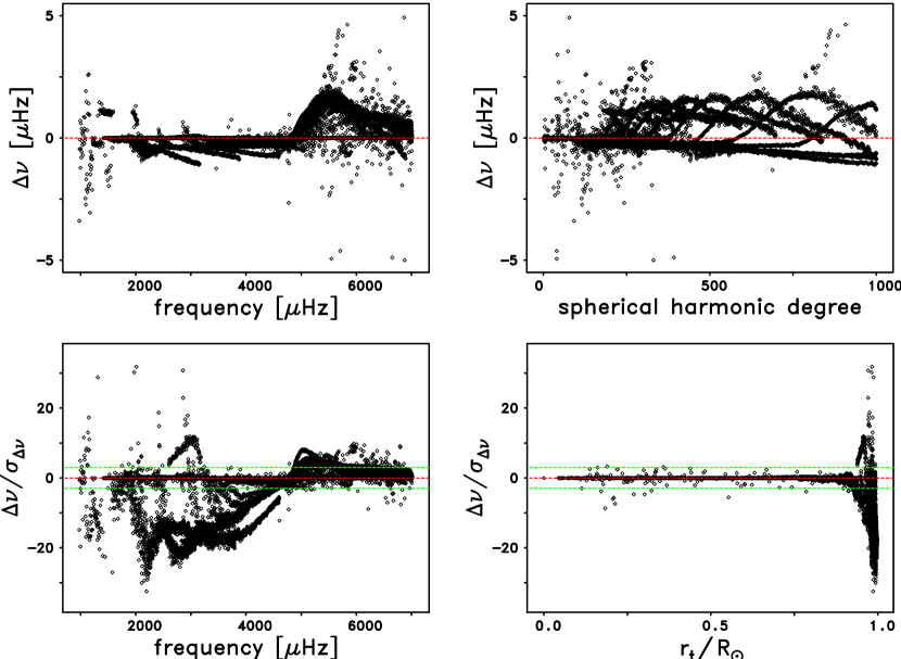
Figure 11: Same as Figure 10, except that it shows the dependence of both the raw and normalized frequency differences, $\Delta\nu$, which resulted from frequency tables $\cal{F}$2010_66c and $\cal{F}$2010_66d, in the sense of “corrected” minus “raw” with respect to frequency, degree, and fractional inner turning-point radius.

5.1.3 Influence of non-n-averaged frequency-splitting coefficients

The influence upon the fitted frequencies of the use of non-$n$-averaged frequency-splitting coefficients in the generation of $m$-averaged power spectra is illustrated in Figure 12. The raw frequency differences, in the sense of “non-$n$-averaged” minus “$n$-averaged”, are shown as functions of frequency and degree in the upper-left and upper-right panels, respectively. These frequency differences resulted when we subtracted the frequencies in table $\cal{F}$2010_66b from those in table $\cal{F}$2010_66d. The principal difference between these raw frequency differences and those shown in the upper panels of Figure 11 is the absence of the strong, wave-like frequency dependence of the high-frequency cases that was seen at the right side of the upper-left panel of Figure 11. It was this wave-like behavior of the high-frequency differences that was also visible as the series of shifted peaks that are visible in the upper-right panel of Figure 11. Hence, the absence of such a similar wave-like variation in the high-frequency differences that are shown in the upper-left panel of Figure 12 resulted in the absence of a similar series of shifted peaks in the upper-right panel of Figure 12. In turn, the absence of this series of positive peaks in the upper-right panel of Figure 12 meant that the majority of the high-degree frequency differences that are shown in the upper-right panel of Figure 12 were negative.

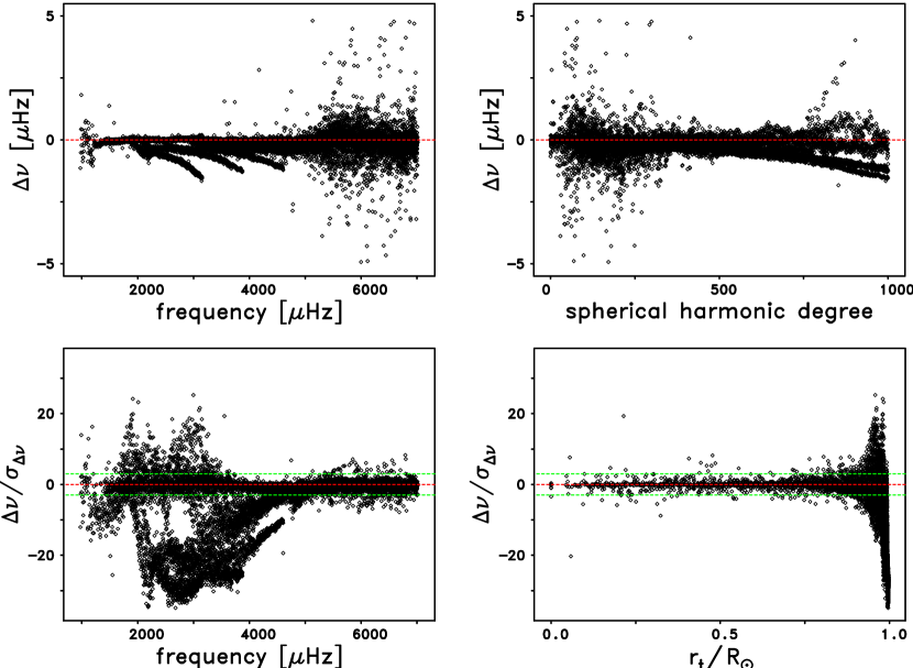
Figure 12: Same as Figure 10, except that it shows the dependence of both the raw and normalized frequency differences, $\Delta\nu$, which resulted from frequency tables $\cal{F}$2010_66b and $\cal{F}$2010_66d, in the sense of “non-$n$-averaged” minus “$n$-averaged” with respect to frequency, degree, and fractional inner turning-point radius.

The frequency dependence of the normalized frequency differences that resulted from the use of the non-$n$-averaged frequency-splitting coefficients is shown in the lower-left panel of Figure 12. Close comparison of this panel with the corresponding panel of Figure 11 illustrates that both sets of normalized frequency differences had a very similar frequency dependence. As was the case in Figure 11, the most significant of these normalized frequency differences were negative and corresponded to $\nu<4500\,\,\mu$Hz.

The dependence of the subset of the normalized frequency differences for which $\nu<4500\,\,\mu$Hz upon the fractional inner turning-point radius is shown in the lower-right panel of Figure 12. As was the case in Figure 11, the most significant subset of these normalized frequency differences was concentrated in the outer portion of the convection zone. Very few of the normalized frequency differences that had inner turning-point radii inward of $0.875\,R_{\odot}$ were outside the range of $\pm 3\,\sigma$.

The statistics of both the raw and normalized frequency differences are given in section C3 (i.e., rows 5 and 6) of Table 5. Here, we can see in row 6 that the average magnitude of the normalized frequency differences for the frequency range $\nu<7000\,\,\mu$Hz was equal to $5.8\,\sigma$, while the average magnitude of the normalized frequency differences for the cases for which $\nu<4500\,\,\mu$Hz was equal to $10.2\,\sigma$. Comparison of both averages with those for the same frequency range in row 4 of Table 5 shows that the effects of using non-$n$-averaged splitting coefficients were only slightly more significant than were the effects of the correction of the raw frequency splitting coefficients. Other than this minor difference, the influence of the non-$n$-averaged splitting coefficients upon the fitted frequencies was very similar to that of the correction of the raw frequency splitting coefficients themselves.

We have just shown in both Figure 12 and in section C3 (i.e., rows 5 and 6) of Table 5 that the use of corrected, non-$n$-averaged splitting rather than the corrected, $n$-averaged splitting coefficients in the generation of the $m$-averaged power spectra produced significant frequency differences for the low-order ridges. In order to determine which ridges were most sensitive to the changes in the splitting coefficients due to the use of non-$n$-averaged coefficients, we compared the differences between the frequencies in Tables $\cal{F}$2010_66b and $\cal{F}$2010_66d with the differences in the two sets of corrected splitting coefficients themselves, and we found that the use of the $n$-averaged splitting coefficients was equivalent to using only the splitting coefficients of the higher-order ridges in the generation of the $m$-averaged spectra. The use of the non-$n$-averaged splitting coefficients for the low-order ridges is what resulted in the introduction of the significant, systematic frequency differences.

5.2 Sensitivity of Method 2 to an increase in the widths of leakage matrix peaks

In addition to studying the influence on the fitted frequencies of the details of the computation of the $m$-averaged power spectra, we also investigated the effects of an increase in the width of the Gaussian approximation that we employ to represent the peaks of the leakage matrices (cf. Section 4.1). To this end, we refitted the $m$-averaged spectral set $\cal{S}$2010_66b with the Method 2 code using a Gaussian approximation the width of which has been increased artificially by 18 %. This fitting run resulted in the frequency table $\cal{F}$2010_66b.lkm. By subtracting the frequencies in table $\cal{F}$2010_66b from those in table $\cal{F}$2010_66b.lkm we obtained raw frequency differences the frequency and degree dependencies of which are shown, in the sense of “wider Gaussian” minus “original Gaussian”, in the upper-left and upper-right panels, respectively, in Figure 13. Comparison of these two panels with the upper panels of Figure 10 shows that these raw frequency differences were similar to those shown in Figure 10, with the main differences being an increase in the number of cases at both high frequencies and moderate degrees for which $\Delta\nu$ was positive and a corresponding decrease in the number of cases for which $\Delta\nu$ was negative. Further comparison of the two upper panels of Figure 13 with the upper panels of both Figures 11 and 12 shows that the increase in the width of the leakage matrix peak did not result in systematic frequency differences for the low-order ridges.

The normalized frequency differences that resulted from the use of the different approximations to the peaks of the leakage matrices are shown in the lower-left panel of Figure 13. Comparison of this panel with the lower-left panel of Figure 10 confirms the absence of any significant frequency differences in both figures. The dependence of the subset of the normalized frequency differences for which $\nu<4500\,\,\mu$Hz upon the fractional inner turning-point radius is shown in the lower-right panel of Figure 13. This panel demonstrates that, with the exception of a small concentration of significant differences just below the photosphere, there is no obvious radial dependence to the remaining differences that exceeded $\pm 3\,\sigma$.

The statistics of the frequency differences that are shown in Figure 13 are summarized in section C4 of Table 5. Here, row 7 shows that the average magnitude of the raw frequency differences was $0.149\,\,\mu$Hz for the cases for which $\nu<7000\,\,\mu$Hz and dropped to $0.060\,\,\mu$Hz for the cases for which $\nu<4500\,\,\mu$Hz, while row 8 confirms our statement above that these frequency differences were not significant, since the average ratio was equal to 1.00 over the entire frequency range, and was equal to only 1.37 for the low-frequency subset.

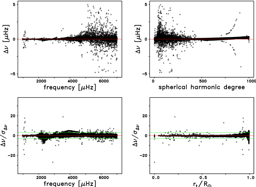
Figure 13: Same as Figure 10, except that it shows the dependence of both the raw and normalized frequency differences, $\Delta\nu$, which resulted from frequency tables $\cal{F}$2010_66b and $\cal{F}$2010_66b.lkm, in the sense of “wider Gaussian” minus “original Gaussian” with respect to frequency, degree, and fractional inner turning-point radius.

6 Sample results from Method 2 and comparison with Method 1

Before we shall present sample results from Method 2 in Section 6.2, we will demonstrate in Section 6.1 the substantial improvements that Method 2 makes in the frequencies, linewidths, and amplitudes that we generated with this method by comparing them with corresponding quantities that we generated using our Method 1. For a description of Method 1 we refer the reader to Appendix A.

6.1 Comparison of results from Methods 1 and 2

One key difference between Method 1 and our Method 2 is the fact that Method 1 is restricted to use only symmetric Lorentzian profiles, while Method 2 includes the option of using either symmetric or asymmetric profiles. A second key difference between the two methods is the use of both narrow and wide fitting ranges in Method 1, while such wide fitting ranges are never employed in Method 2. Instead, in Method 2 we employ the procedure described in Section 4.3 to determine the width of each fitting box individually. As a result, the widths of the fitting boxes vary systematically as functions of both the degree and the frequency in Method 2.

In the three left-hand panels of Figure LABEL:F2, we compare the fitted profiles that Method 1 produced with segments of three different spectra from our $m$-averaged spectral set $\cal{S}$2010_66a. In the three right-hand panels of the same figure we compare the profiles that Method 2 produced for the same three spectral segments using the asymmetric profile of Nigam & Kosovichev (1998). The normalized comparison of Method 1 and Method 2 fit results shown in Table 6 for the same three modes whose fits are shown in Figure LABEL:F2 demonstrates that the Method 2 frequencies and linewidths do agree more closely with the Method 1 results that were computed using the narrow fitting range than they do with the Method 1 results that were computed using the wide fitting range. Table 6 also shows that, with the exception of the frequency that was computed for the $(n,l)=(2,70)$ mode using the narrow fitting range in Method 1, all of the other frequencies and linewidths are systematically different between Method 1 and Method 2.

In Figure 14 we illustrate the improvements that Method 2 made in both the formal frequency and linewidth uncertainties relative to the corresponding quantities that were computed using Method 1. In the upper-left panel of Figure 14 we show the frequency dependence of the ratios of the Method 1 and Method 2 frequency uncertainties for the cases in which the narrow fitting range was employed in Method 1, while we show the frequency dependence of the similar ratios for the cases in which the wide fitting range was employed in the upper-right panel. The average ratio of the two sets of uncertainties in the upper-left panel of this figure was $36.1\pm 1.5$, while the average ratio of the two sets of uncertainties in the upper-right panel was $9.7\pm 0.1$.

The frequency dependence of the ratios in the Method 1 and Method 2 linewidth uncertainties are shown in the lower-left panel of Figure 14 for the cases in which the narrow fitting range was used in Method 1, and we show the frequency dependence of the ratios of the Method 1 and Method 2 linewidth uncertainties for the cases in which the wide fitting range was employed in the lower-right panel of the same figure. The average ratio of the two sets of linewidth uncertainties in the lower-left panel was $96.2\pm 4.3$, while the average ratio of the two sets of linewidth uncertainties in the lower-right panel was $12.6\pm 0.1$. Combining both the narrow and wide fitting range ratios in overall sets of uncertainty ratios, we found that Method 2 reduced the frequency uncertainties by an average ratio of $15.2\pm 0.3$ and it reduced the linewidth uncertainties by an average ratio of $29.8\pm 0.9$. These sizeable reductions in both the frequency and linewidth uncertainties testify to the importance of including more than a single peak in the theoretical profile that is used to fit both modes and ridges of power.

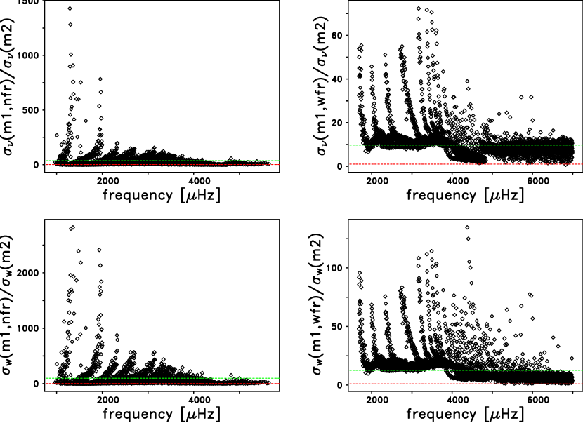
Figure 14: (upper-left) Frequency dependence of the ratios of the Method 1 narrow fitting range frequency uncertainties divided by the Method 2 frequency uncertainties. (upper-right) Frequency dependence of the ratios of the Method 1 wide fitting range frequency uncertainties divided by the Method 2 frequency uncertainties. (lower-left) Frequency dependence of the ratios of the Method 1 and Method 2 linewidth uncertainties for the narrow fitting range cases. (lower-right) Frequency dependence of the ratios of the Method 1 and Method 2 linewidth uncertainties for the wide fitting range cases. In all four panels the dashed green lines show the average ratios, while the dashed red lines show the error ratios of unity. Note that the vertical scales are different in all four panels. In all four panels the $m$-averaged spectral set $\cal{S}$2010_66a has been fitted.

In the upper two panels of Figure 15 we show the improvements that Method 2 introduced into the frequencies of the $n$=0 ridge in comparison with the frequencies computed using Method 1. We demonstrate these improvements by comparing both sets of fitted frequencies with theoretical frequencies that have been computed from Model S of Christensen-Dalsgaard et al. (1996) employing the approach described by Kosovichev (1999). Specifically, in both of these panels we show the frequency dependence of the frequency differences $\Delta\nu=\nu^{\rm obs}-\nu^{\rm mod}$, where $\nu^{\rm obs}$ refers to either our Method 1 or Method 2 fitted frequencies and where $\nu^{\rm mod}$ is the corresponding theoretical frequency computed using Model S. The $\Delta\nu$ values for the Method 1 fits are shown as the black diamonds, while the $\Delta\nu$ values for Method 2 are shown as the red diamonds. The upper-left panel is for the portion of the $n=0$ ridge that was originally fit using the narrow fitting range in Method 1, while the upper-right panel is for the frequency range of the same ridge that was initially fit using the wide fitting range in Method 1. The upper-left panel shows that the Method 2 frequencies are much smoother than the Method 1 frequencies and that they also agree more closely with the theoretical frequencies. The upper-right panel shows that, with the exception of a range of frequencies around $2700\,\,\mu$Hz, the Method 2 frequencies agreed more closely with the theoretical frequencies than did the Method 1 frequencies.

In the lower-left panel of Figure 15 we show the improvements that Method 2 introduced into the linewidths of the $n=0$ ridge. Since there are no theoretical linewidths that we can compare the fitted linewidths with, we have simply plotted both sets of fitted linewidths as a function of frequency in this panel. This comparison demonstrates that the Method 2 linewidths (shown as the red diamonds) varied in a much smoother manner with increasing frequency than did the Method 1 linewidths (shown as the black diamonds). It also demonstrates that for the majority of the modes shown, the Method 2 linewidths were smaller than were the corresponding linewidths computed using Method 1.

In the lower-right panel of Figure 15 we extend our comparison of the Method 1 and Method 2 linewidths to the entire set of 30 ridges that were fit using Method 2 and using both fitting ranges in Method 1. Here we have plotted the frequency dependence of the ratios of the Method 2 linewidths divided by the Method 1 linewidths. This panel clearly shows that for all of the modes with frequencies below the acoustic cut-off frequency the fits computed using Method 2 produced linewidths that were smaller than the corresponding Method 1 linewidths by factors ranging between 2 and 5. The smaller linewidths all correspond to longer estimated lifetimes for these modes.

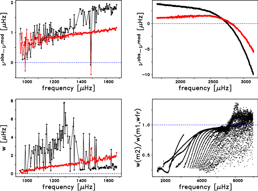
Figure 15: (upper-left) Frequency dependence of two sets of frequency differences, $\Delta\nu=\nu^{\rm obs}-\nu^{\rm mod}$, between our fitted frequencies, $\nu^{\rm obs}$, and the corresponding Model S frequencies, $\nu^{\rm mod}$, for the $n=0$ ridge. The $\Delta\nu$ values as computed by Method 1 using the narrow fitting range are shown as the black line, while the $\Delta\nu$ values computed using Method 2 are shown as the red line. The outlier in both the Method 1 and Method 2 frequencies at about $1500\,\,\mu$Hz is for $l=219$, and is caused by a glitch in the underlying spectrum. In both upper panels the dashed blue line represents a difference of zero. (upper-right) Same as upper-left panel, except that the wide fitting range was used for computing the Method 1 frequencies. (lower-left) Frequency dependence of the linewidths computed using Method 1 with the narrow fitting range (the black line) and using Method 2 (the red line). The dashed blue line represents linewidths of zero. (lower-right) Frequency dependence of the ratio of the linewidths as computed using Method 2 divided by the linewidths computed using Method 1 with the wide fitting range. The dashed line represents a linewidth ratio of unity. In all four panels, the fits were computed using the $m$-averaged spectral set $\cal{S}$2010_66a.

in order to show the entire frequency range spanned by both fitting ranges with a common scale for the y-axis”

In the upper-left panel of Figure LABEL:dfm1ms we have combined both portions of our comparisons of Method 1 and Method 2 frequencies with the Model S frequencies for the $n=0$ ridge into a single panel in order to show the entire frequency range spanned by both fitting ranges with a common scale for the vertical axis to illustrate yet another important improvement of Method 2 over Method 1 – namely the complete absence in the Method 2 frequencies of the substantial discontinuity that is present in the Method 1 frequencies at precisely the frequency where the transition was made from the use of the narrow fitting range to the use of the wide fitting range in that method. In the upper-right panel of Figure LABEL:dfm1ms we show a similar comparison of Method 1 and Method 2 frequencies with the corresponding Model S frequencies for the $n=1$ ridge. As with the upper-left panel, there is a pronounced discontinuity in the Method 1 frequencies at the location of the switch-over from the narrow fitting range to the wide fitting range that is absent in the Method 2 frequencies.

In addition to the introduction of jumps into the fitted frequencies, the switch-over in the width of the fitting ranges that were employed in Method 1 also caused a corresponding discontinuity in the Method 1 linewidths, as we show here in the two middle panels of Figure LABEL:dfm1ms. The jumps in the linewidths that are shown in black in these two panels occurred for exactly the same modes for which the frequencies also exhibited the jumps in the two upper panels. In contrast to the Method 1 linewidths, the Method 2 linewidths exhibited no such discontinuities, as we show in red in the middle panels of Figure LABEL:dfm1ms. As we also showed in the lower panels of Figure 15, the Method 2 linewidths agreed more closely with the Method 1 linewidths that were computed using the narrow fitting range than they did with the Method 1 linewidths that were computed using the wide fitting range.

We also demonstrate in the two lower panels of Figure LABEL:dfm1ms that the use of the single-peak profile in Method 1 introduced discontinuities in the amplitudes (as shown in black), or power densities, that disappeared when the multiple-peak profile of Method 2 was used instead (as shown in red). Not only did the single-peak profile introduce discontinuities into the amplitudes, it also caused the amplitudes that were computed using the narrow fitting range to show more scatter as a function of degree along the ridges to the left of the jumps than was the case with our Method 2 amplitudes.

In Figure LABEL:m1ridgejumps we demonstrate that the replacement of the narrow fitting range with the wide fitting range in Method 1 did not just introduce distinct discontinuities in the fitted frequencies, linewidths, and amplitudes for the $n=0$ and $n=1$ ridges, but rather introduced similar discontinuities in all three quantities for nearly all of the ridges that we fit. We found it useful to measure these discontinuities in terms of the normalized discontinuities defined as

$$\delta\varUpsilon(l_{1},l_{2})/\varSigma_{\Delta\varUpsilon},$$ (42)

where $\varUpsilon$ can be either frequency $\nu$, linewidth $w$, or else the logarithm of the amplitude $A$, and where

$$\delta\varUpsilon(l_{1},l_{2})=\Delta\varUpsilon(l_{2})-\Delta\varUpsilon(l_{1})=\varUpsilon^{\rm\,fit}(l_{2})-\varUpsilon^{\rm\,seed}(l_{2})-\left[\varUpsilon^{\rm\,fit}(l_{1})-\varUpsilon^{\rm\,seed}(l_{1})\right],$$ (43)

with $l_{1}$ being the degree of the highest-degree mode that we fit using the narrow fitting range for a given ridge, with $l_{2}$ being the degree of the lowest-degree mode that we fit using the wide fitting range for the same ridge, and with $\varUpsilon^{\rm\,fit}$ and $\varUpsilon^{\rm\,seed}$ denoting, respectively, the fitted and the corresponding seed value of $\varUpsilon$, and where $\varSigma_{\Delta\varUpsilon}$ is the point-to-point scatter in the $\Delta\varUpsilon$ values for the same ridge, as computed from equation (B1) using

$$\upsilon\equiv\Delta\varUpsilon/\Delta l,$$ (44)

with $\Delta\varUpsilon=\varUpsilon^{\rm\,fit}-\varUpsilon^{\rm\,seed}$. The use of the differences $\varUpsilon^{\rm\,fit}-\varUpsilon^{\rm\,seed}$ rather than the fitted values, $\varUpsilon^{\rm\,fit}$, themselves in the above equations (43) and (44) has the advantage that the changes $\Delta\varUpsilon/\Delta l$ are approximately zero along the ridge under consideration and, thus, gives rise to an unbiased value of the scatter, $\varSigma_{\Delta\varUpsilon}$, as pointed out in Appendix B1. We note that the values of $\varUpsilon^{\rm\,seed}$ that we have employed are smoothly varying with degree, and we also note that we used a different pair of $l_{1}$ and $l_{2}$ values for each of the analyzed ridges, depending on the degree at which the narrow fitting range is replaced with the wide fitting range in Method 1.

In the upper-left panel of Figure LABEL:m1ridgejumps we show the normalized discontinuities, $\delta\nu(l_{1},l_{2})/\varSigma_{\Delta\nu}$, in both the Method 1 and Method 2 frequencies in dependence of the radial order $n$. These normalized discontinuities were computed from equations (42) through (44) using $\varUpsilon\equiv\nu$, with $\nu$ denoting the fitted frequency from either Method 1 or Method 2. The hereto required values of the seed frequency, $\nu^{\rm seed}$, were taken from a suitable seed table (cf. Section 4.2). In order to help indicate which of the normalized frequency discontinuities represent statistically significant values, we have included the two dashed green lines at ratios of $\pm 3$. Inspection of the upper-left panel of Figure LABEL:m1ridgejumps shows that for Method 1 (black diamonds) 14 of the 30 normalized frequency discontinuities exceeded $\pm 3\,\sigma$. By contrast, of the 30 normalized frequency discontinuities that we generated using Method 2, and which are shown as the set of red triangles in the upper-left panel of Figure LABEL:m1ridgejumps, none of them exceeded $\pm 3\,\sigma$. Clearly, the multiple-peak profile that we are using in Method 2 has allowed us to overcome the discontinuities that we were forced to introduce into the fitted frequencies when we were using the single-peak profile of Method 1.

The introduction of the jumps into the Method 1 frequencies that corresponded to the change-over in the fitting range that we had to employ with Method 1 meant that those frequencies could not be employed in structural inversions since these jumps would introduce unphysical oscillations in the radial profile of any quantity determined in such inversions, e.g., internal sound speed. We have re-plotted the normalized Method 1 frequency discontinuities that are shown in the upper-left panel of Figure LABEL:m1ridgejumps as a function of the inner turning-point radius of the $l_{1}$ mode in the upper-right panel of Figure LABEL:m1ridgejumps. It is clear from this panel that one group of significant Method 1 frequency discontinuities corresponds to modes that span the lower portion of the convection zone, while the other group of statistically significant discontinuities corresponds to modes that span the sub-surface shear layer. On the other hand, the fact that none of the 30 normalized frequency discontinuities computed using Method 2 exceeded $\pm 3\,\sigma$ means that this method is capable of producing frequencies that can be employed in successful structural inversions, as we will show later in section 7.

For the linewidths, as shown in the lower-left panel of Figure LABEL:m1ridgejumps, 23 of the 30 normalized Method 1 discontinuities, $\delta w(l_{1},l_{2})/\varSigma_{\Delta w}$, exceeded $\pm 3\,\sigma$, while only the $n=0$ value exceeded $\pm 3\,\sigma$ for Method 2. For the logarithm of the amplitudes, as shown in the lower-right panel of Figure LABEL:m1ridgejumps, 21 of the 30 normalized Method 1 discontinuities, $\delta\log A(l_{1},l_{2})/\varSigma_{\Delta\log A}$, exceeded $\pm 3\,\sigma$. However, none of the normalized Method 2 discontinuities exceeded $\pm 3\,\sigma$. Clearly, Method 2 is able to produce both linewidths and amplitudes which do not exhibit the systematic discontinuities that Method 1 introduced into both quantities.

In addition to all of the discontinuities in the frequencies, linewidths, and amplitudes, Method 1 also introduced similar discontinuities into the frequency uncertainties, as we show in both panels of Figure 16. In these panels we show the frequency dependence of the logarithm of the Method 1 frequency uncertainties that were computed from the fits to the $m$-averaged spectral set $\cal{S}$2010_66a as the black curves. The left-hand panel is for the $n=1$ ridge, while the right-hand panel is for the $n=2$ ridge. There are clearly discontinuities in both curves at the locations of the vertical dashed lines, which are located at the frequencies of the transition from the narrow fitting range to the wide fitting range for both ridges. By contrast, the corresponding frequency uncertainties that we computed for the same power spectra for both of these ridges using Method 2 are shown as the two red curves. It is clear that neither of these curves contains a discontinuity at the location of the vertical lines.

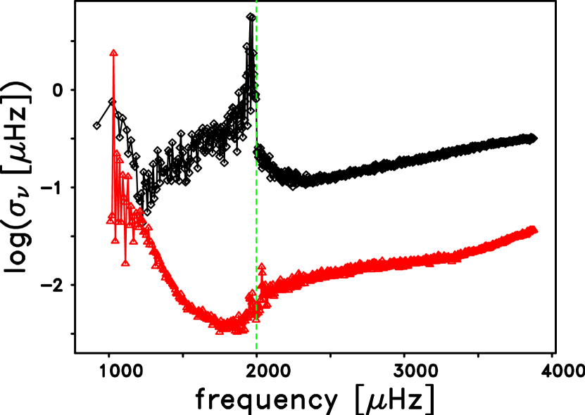
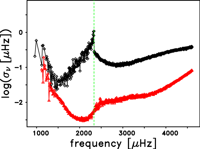
Figure 16: (left) The frequency dependence of the logarithm of the Method 1 frequency uncertainties for the $n=1$ ridge is shown as the black curve, while the frequency dependence of the logarithm of the corresponding Method 2 uncertainties is shown as the red curve. The vertical dashed line denotes the frequency where the wide fitting range replaced the narrow fitting range in Method 1. (right) Same as the left panel, except that the two sets of frequency uncertainties were for the $n=2$ ridge. Both sets of these frequency uncertainties resulted from fits to the $m$-averaged spectral set $\cal{S}$2010_66a.

6.2 Sample results from Method 2

The results that we will now describe were obtained from fitting the $m$-averaged spectral sets $\cal{S}$2010_66a and $\cal{S}$2010_03 using Method 2. These two spectral sets have been computed from the 66-day long observing run $\cal{R}$2010_66 and from the 3-day long observing run $\cal{R}$2010_03, respectively. The rationale behind the fitting of spectra from both a 66-day long time series and a 3-day long time series is to investigate the impact of spectral resolution upon the performance of Method 2. In each of these two sets of $m$-averaged spectra we considered modes in the range $0\leq l\leq 1000$, $0\leq n\leq 29$, $900\leq\nu\leq 7000\,\,\mu$Hz. In this range of frequencies, radial orders, and degrees the seed table that we had available to us contained a total of 12,533 entries.

In the low-degree, low-frequency portion of the dispersion plane, the mode amplitude becomes comparable to the background noise, and at the same time the mode linewidth becomes smaller than the spectral resolution. This can easily lead to the confusion of a noise spike with a modal peak. By a careful inspection of the quality of the fits we therefore set, for each radial order, $n$, a lower degree limit, $l_{\rm min}^{(n)}$, below which we did not try to fit a mode for that ridge. In a similar analysis of the high-degree, high-frequency portion of the dispersion plane we defined, for each ridge, an upper degree limit, $l_{\rm max}^{(n)}$, above which we did not try to fit a mode for that ridge. Based upon this approach we came up with a total of 12,359 modes to be fit for the 66-day spectra, and a slightly smaller total of 12,242 modes to be fit for the 3-day spectra because of the lower signal-to-noise ratios present in this set of spectra. We found that for all of the modes that we attempted to fit in the case of the 66-day spectra and the 3-day spectra, respectively, the Method 2 code converged on a solution. As a result, we ended up with a total of 12,359 sets of fitted mode parameters for the 66-day spectra, and a total of 12,242 sets of fitted mode parameters for the 3-day spectra. This impressively demonstrates that Method 2 is working in a stable manner over wide ranges of frequency, degree, and spectral resolution.

We collected the 12,359 frequencies and their corresponding uncertainties that we generated with Method 2 from the $\cal{S}$2010_66a $m$-averaged power spectra into the frequency table $\cal{F}$2010_66a (cf. Section 5.1). The dispersion plane coverage of this set of frequencies is illustrated in Figure 17. For the reasons explained in Section 4.6, we employed the symmetric Lorentzian profile for fitting the pseudo-modes. For all of the cases for which the Lorentzian profile was used, the line asymmetry was defined to be zero, i.e., $B=0$. Those cases are shown as the red diamonds in Figure 17. For all of the other cases, which are shown as the black diamonds, the asymmetric profile of Nigam & Kosovichev (1998) was employed.

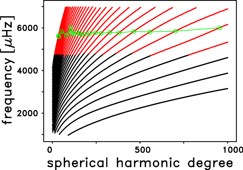
Figure 17: Dispersion plane coverage of the set of frequencies obtained with Method 2 when applied to the $m$-averaged spectral set $\cal{S}$2010_66a. In the range $0\leq l\leq 1000$, $0\leq n\leq 29$, $965\leq\nu\leq 7000\,\,\mu$Hz we were able to successfully fit a total of 12,359 modes. The black diamonds are for fits employing the asymmetric profile of Nigam & Kosovichev (1998), while the red diamonds are for those fits for which the symmetric Lorentzian profile was used. The frequencies where the linewidths of most of the ridges exhibited either local or global maxima are shown as the green open circles that are connected by the green solid line. All of these frequencies can be seen to lie above the corresponding frequencies where the fitting profiles were switched. The maxima in the linewidths are shown as a function of frequency in the upper-left panel of Figure 18, while the maximum in the $n=14$ ridge is shown in the upper-right panel of Figure 19.

In addition to the frequencies that we computed from the $\cal{S}$2010_66a $m$-averaged power spectra using Method 2, we show the corresponding linewidths and line asymmetries in the upper-left and lower-left panels of Figure 18, respectively. The upper-left panel shows that the linewidths of the higher-order ridges exhibited either local or global maxima for frequencies between 5800 and $6000\,\,\mu$Hz before decreasing slightly at higher frequencies. The frequencies where the linewidths of the ridges exhibited either local or global maxima are shown as the green open circles in Figure 17 that are connected by the solid green line. All of these frequencies can be seen to lie well above the range of frequencies where the fitting profile was switched from an asymmetric to a symmetric profile, which was $4638<\nu<4842\,\,\mu$Hz.

The maxima in the linewidths are very similar to peaks in the high-frequency linewidths that were shown in Figure 4 of Duvall et al. (1991). If we compare the frequencies of the peaks in the linewidths in the degree range that they employed (i.e., $11\leq l\leq 150$) with the frequencies as given by the green line in Figure 17, we see that our frequencies are about $200\,\,\mu$Hz larger than the frequencies given by Duvall et al. (1991). This small difference is most likely due to the different levels of solar activity in the two observing epochs. The Duvall et al. (1991) observations were acquired in late 1987, while the 66-day data set that we have employed, viz. $\cal{S}$2010_66a, was acquired in mid-2010. We find it intriguing that the solid green line that connects the maxima in the linewidths in Figure 17 looks very similar to the degree dependence of the chromospheric modes as shown in Figure 5 of Ulrich & Rhodes (1977); however, the frequencies of these linewidth maxima are all much closer to the frequency of the second chromospheric mode, which Ulrich & Rhodes (1977) computed to be $5570\,\,\mu$Hz than they are to the frequency of the first mode, which they computed to be $4138\,\,\mu$Hz. Furthermore, there is no evidence in Figure 18 for the first chromospheric mode in the linewidths, nor is there any evidence in Figure 17 for either chromospheric mode in the frequencies themselves. Since there is no other evidence for either chromospheric mode in any of our frequency tables, the origin of these local maxima in the linewidths is not clear, but is probably related to the transition from standing waves below the acoustic cut-off frequency to pseudo-modes above. The lower-left panel of Figure 18 shows that most of the line asymmetries were negative, while they were zero by construction for those cases for which the symmetric Lorentzian profile was used in Method 2.

The amplitudes, or power densities, as is shown in the upper-right panel of Figure 18, peak very close to $3000\,\,\mu$Hz, in agreement with all previous studies of the solar oscillation amplitudes. In contrast, the power values that are shown in the lower-right panel go through their peak at about $3300\,\,\mu$Hz because the power values are computed from the products of the amplitudes and the linewidths and the increase in the linewidths with increasing frequency partially compensates for the decreasing amplitudes. As we summarized at the beginning of this section, we also obtained similar sets of linewidths, line asymmetries, amplitudes, and power values for the set of 3-day power spectra in addition to the results we have shown in this section from the 66-day power spectra.

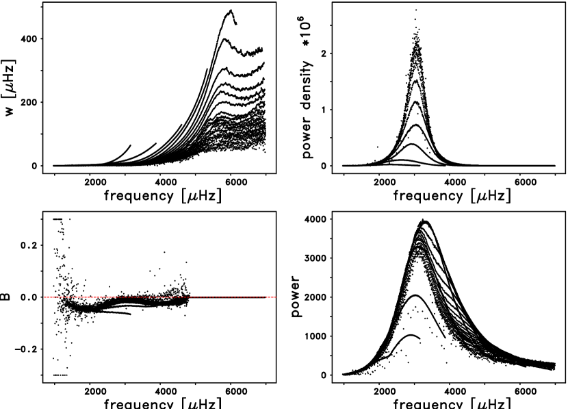
Figure 18: The frequency dependencies of the linewidths (upper-left), line asymmetries (lower-left), amplitudes, or power densities (upper-right), and powers (lower-right) of the 12,359 fits that were made using Method 2 on the $m$-averaged spectral set $\cal{S}$2010_66a. The linewidths of many of the ridges exhibit either local or global maxima near frequencies around 5800 to $6000\,\,\mu$Hz before decreasing slightly at even higher frequencies. For $\nu<4638\,\,\mu$Hz, only the asymmetric profile was used and the vast majority of the line asymmetries were less than zero. For reasons described in Section 4.6, for $4638<\nu<4842\,\,\mu$Hz, the asymmetric profile was used for some of the ridges, while the symmetric Lorentzian profile was employed for others. For $\nu>4842\,\,\mu$Hz only the symmetric profile was used, so $B$ was set equal to zero for all of those cases. The dashed red line in the lower-left panel is for a line asymmetry $B=0$.

The smoothness in both the fitted frequencies and linewidths that resulted from the fits to the $\cal{S}$2010_66a $m$-averaged power spectra using Method 2 is illustrated in Figure 19 using the example of the $n=14$ ridge. The upper-left panel shows the degree dependence of the frequencies for that ridge, and it also includes the smooth fit to those frequencies as the red curve. The lower-left panel shows the degree dependence of the frequency slope, $\Delta\nu/\Delta l$, that was computed as described in the figure caption, and it also includes, as the blue curve, the derivative with respect to degree of the red curve shown in the upper-left panel. The fact that the derivative with respect to degree (blue line in the lower-left panel) of the smooth curve (red line in the upper-left panel) fitted to the frequencies is an excellent representation of the numerical values of $\Delta\nu/\Delta l$ (black diamonds in lower-left panel) at all of the degrees shown, impressively demonstrates the smoothness of the fitted frequencies (black diamonds in upper-left panel). The upper-right panel of Figure 19 shows the degree dependence of the linewidths for the $n=14$ ridge, and it also includes the smooth fit to those linewidths as the red curve. This panel shows that this ridge was one of the ridges for which the linewidth exhibited a local maximum before decreasing toward the high-degree ends of those ridges as we just described in Figure 18. The lower-right panel of Figure 19 shows the linewidth slopes, $\Delta w/\Delta l$, which were computed as described in the figure caption, as a function of degree, and it also includes, as the blue curve, the derivative of the smooth curve with respect to degree that is shown as the red curve in the upper-right panel. As was the case for the frequencies, the linewidths are also smooth enough that the derivative of the smooth fitting curve provides an excellent representation to the values of $\Delta w/\Delta l$.

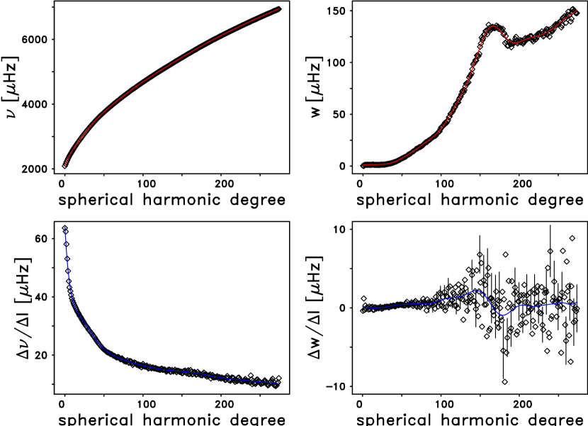
Figure 19: (upper-left) Degree dependence of frequency, $\nu$, for the $n=14$ ridge from fitting the $m$-averaged spectral set $\cal{S}$2010_66a using Method 2. The black diamonds represent the fitted frequencies in the range $0\leq l\leq 274$. The red line is for a smooth fit to these fitted frequencies. (lower-left) Degree dependence of the frequency slopes, $\Delta\nu/\Delta l$, for the same ridge. The values of $\Delta\nu/\Delta l$ are plotted as the black diamonds at the abscissae $l+0.5$, and are computed by subtracting two consecutive values of the fitted frequency shown in the upper-left panel, i.e., $\Delta\nu/\Delta l|_{l+0.5}=\nu(l+1)-\nu(l)$. The blue line is the derivative with respect to $l$ of the smooth curve that has been fitted to the frequencies and which is shown as the red line in the upper-left panel. (upper-right) Degree dependence of the modal linewidth, $w$. We note that the linewidth goes through a relative maximum at $l\approx 167$ which corresponds to a frequency of $5686\,\,\mu$Hz. This is an example of the linewidth maxima that were illustrated in Figure 18. (lower-right) Degree dependence of the linewidth slopes, $\Delta w/\Delta l$, plotted as the black diamonds at the abscissae $l+0.5$. They were computed by subtracting two consecutive values of the fitted linewidth, i.e., $\Delta w/\Delta l|_{l+0.5}=w(l+1)-w(l)$. The blue line is the derivative of the smooth curve that has been fitted to the linewidths and which is shown as the red line in the upper-right panel.

As we noted in Section 4.2, the derivatives with respect to degree of the frequency, the linewidth, and the amplitude are an essential ingredient of Method 2. We compute these derivatives on a ridge-by-ridge basis by fitting, as a function of degree, higher-order Chebyshev polynomials to the frequencies, linewidths, and amplitudes, respectively, as they have been determined with Method 2, and by then differentiating the resulting polynomials with respect to degree. The red curves in the upper panels of Figure 19 are examples of such fits to the frequency and linewidth, respectively, while the blue curves shown in the lower panels are examples of the first derivative of the fitted polynomials. Because higher-order polynomials are involved, this approach is prone to deliver wildly oscillating fitting curves. Therefore, the degree of the polynomials has to be selected rather carefully, and the least-squares fits of the polynomials need to be constrained as to avoid oscillating curves.

7 Helioseismic inversion for solar structure

In this Section we will present the results of an inversion for the radial structure of the Sun using a subset of the frequencies that are contained in our table $\cal{F}$2010_66a. We have already mentioned in Section 6.2 that this entire table contains a total of 12,359 sets of fitted modal parameters, and we showed the dispersion plane coverage of this complete set of frequencies in Figure 17. This is the largest mode-set to have ever been fit thus far in helioseismology. To carry out our structural inversion, we selected a subset of 6,366 frequencies which contained degrees that ranged from 0 to 1000, radial orders from 0 to 29, and frequencies from 969 to $4500\,\,\mu$Hz. Since this frequency upper limit of $4500\,\,\mu$Hz is less than the frequency of the lowest symmetrical fit, which was $4638\,\,\mu$Hz for the $n=17$ ridge, all of the frequencies in this subset were computed using the asymmetric profile of Nigam & Kosovichev (1998). By using the Optimally Localized Averaging (OLA) technique we inverted this subset of modes to determine the spherically symmetric structure of the Sun. We limited the frequency range of the subset of modes by $4500\,\,\mu$Hz because this threshold is well below the acoustic cut-off frequency which separates the $p$-modes from the pseudo-modes and which is about $5000\,\,\mu$Hz. We note that the choice of the upper frequency limit of the mode set to be inverted is not critical since modes with frequency above $4000\,\,\mu$Hz do not contribute significantly to the inversion results due to their large errors. Details of the inversion procedure, including calculation of the sensitivity kernels and test results, are presented by Kosovichev (1999).

While we had to select from our full mode-set a suitable subset of frequencies for our structural inversion, we note, however, that tables of fitted mode parameters covering a similar range of degrees and frequencies as our full mode-set presented here, are an indispensable prerequisite for the study of temporal changes in the sensitivities of the mode parameters to corresponding changes in the levels of solar activity (see, e.g., Rabello-Soares et al., 2008b; Rhodes et al., 2011; Rabello-Soares, 2011).

7.1 Analysis of systematic errors in fitted frequencies and associated uncertainties

In an inversion for solar internal structure both the frequencies and the associated uncertainties of the solar oscillation modes are employed as input parameters. Therefore, systematic errors in these input parameters may affect the resulting inferences of the Sun’s internal structure. As we have explained in Section 3.2.3, such systematic errors may arise from instrumental effects. However, they also are likely to arise from the methodology employed for fitting the spectra. For example, the use of an inadequate fitting box around the target peaks, an inadequate treatment of the background power within the selected fitting boxes, and/or contributions from $n$- and $l$-leaks that are not adequately accounted for in the fitting model profile, as given in equations (26) through (31), may lead to systematic errors in both the fitted frequencies and the uncertainties thereof. On the other hand, the presence of a group of outliers in a table of frequencies and associated uncertainties that is designed to be used as input to a solar structural inversion, may result in the appearance of unphysical oscillations in the radial profiles of the resulting sound speed or other thermodynamic quantities. Such a set of outliers may also have the unwanted side effect of preventing a stable, regularized solution from being found outside of a very narrow range of the regularization parameter that is being employed in the inversion procedure. In order to avoid the appearance of such unphysical oscillations in the inverted sound speed profile, we developed a five-step procedure that allows us to substantially alleviate the issue of systematic errors in both the fitted frequencies and their associated uncertainties in tables that will be employed as input data sets for structural inversions. The rather high complexity of this procedure mainly results from our desire to keep the approach as objective as possible, while keeping unavoidable subjective elements at a minimum.

The basic idea behind our correction scheme is to compare the observed frequency for the $(n,l)$ mode, $\nu_{n,l}^{\rm obs}$, where the term “observed frequency” refers to our original set of fitted frequencies, with the theoretical model frequency for the same mode, $\nu_{n,l}^{\rm mod}$, on a ridge-by-ridge basis. For this comparison we employ two sets of frequency differences between the observed frequencies, $\nu_{n,l}^{\rm obs}$, and the model frequencies, $\nu_{n,l}^{\rm mod}$, viz. the set of unscaled differences,

$$\Delta\nu_{n,l}=\nu_{n,l}^{\rm obs}-\nu_{n,l}^{\rm mod},$$ (45)

and the set of scaled differences

$$\delta\nu_{n,l}=(\nu_{n,l}^{\rm obs}-\nu_{n,l}^{\rm mod})\,q_{n,l}\left(\frac{\nu_{n,l}^{\rm mod}}{1000}\right)^{-3.5}\equiv\Delta\nu_{n,l}\,q_{n,l}\left(\frac{\nu_{n,l}^{\rm mod}}{1000}\right)^{-3.5}.$$ (46)

In equations (45) and (46) $\nu_{n,l}^{\rm mod}$ is the theoretical frequency of mode $(n,l)$ that has been computed from Model S of Christensen-Dalsgaard et al. (1996) employing the approach described by Kosovichev (1999), and $q_{n,l}$ is the inertia of mode $(n,l)$, normalized to the inertia of mode $(n,0)$. We note that both $\nu_{n,l}^{\rm mod}$ and $q_{n,l}$ are computed using the same solar model that is also used to compute the kernel functions employed in the structural inversion. The rationale behind the use of two different sets of frequency differences, $\Delta\nu_{n,l}$ and $\delta\nu_{n,l}$, respectively, is to exploit the fact that, for a given ridge, the run of $\Delta\nu_{n,l}$ with respect to degree differs markedly from that of $\delta\nu_{n,l}$. This allows the identification of outliers that would otherwise remain undetected if only one set of frequency differences is used. The rationale behind the definition of the scaled frequency differences, $\delta\nu_{n,l}$, is to remove the frequency differences between the solar model and the Sun that come from the dominant near-surface effects (e.g., Christensen-Dalsgaard & Gough, 1984) by approximating these differences using a frequency power-law function scaled with the mode inertia.

Before we delve into the details of our correction scheme, we briefly summarize its major steps. First, for each ridge we fit, as a function of degree $l$, a Chebyshev polynomial, $\varXi_{\varpi}^{(n)}(l)$, of degree $\varpi$ to the unscaled frequency differences, $\Delta\nu_{n,l}$, and a Chebyshev polynomial, $\varPi_{\pi}^{(n)}(l)$, of degree $\pi$ to the scaled frequency differences, $\delta\nu_{n,l}$. Although both $\varXi_{\varpi}$ and $\varPi_{\pi}$ are Chebyshev polynomials of the same kind but generally of different degree, we have introduced different symbols for them in order to highlight that they are used for the fitting of different sets of frequency differences.

Next, from the two fit polynomials, $\varXi_{\varpi}^{(n)}(l)$ and $\varPi_{\pi}^{(n)}(l)$, respectively, we generate, for each ridge, two sets of emulated (imitated) frequencies, $\nu_{n,l}^{\rm em1}$ and $\nu_{n,l}^{\rm em2}$, respectively. Here, $\nu_{n,l}^{\rm em1}$ corresponds to an observed frequency that would fall exactly onto the fitted curve $\varXi_{\varpi}^{(n)}(l)$, while $\nu_{n,l}^{\rm em2}$ corresponds to an observed frequency that would fall exactly onto the fitted curve $\varPi_{\pi}^{(n)}(l)$. At this point we have five sets of frequency differences at our disposal, namely,

$$\Delta_{n,l}^{(1)} =\Delta\nu_{n,l}-\varXi_{\varpi}^{(n)}(l),$$ (47)

$$\Delta_{n,l}^{(2)} =\delta\nu_{n,l}-\varPi_{\pi}^{(n)}(l),$$ (48)

$$\Delta_{n,l}^{(3)} =\nu_{n,l}^{\rm obs}-\nu_{n,l}^{\rm em1},$$ (49)

$$\Delta_{n,l}^{(4)} =\nu_{n,l}^{\rm obs}-\nu_{n,l}^{\rm em2},$$ (50)

$$\Delta_{n,l}^{(5)} =\nu_{n,l}^{\rm em1}-\nu_{n,l}^{\rm em2},$$ (51)

from which we identify outlying modes by applying suitable statistical criteria.

Next, we refit, by means of the WMLTP method employing updated seed tables, all of the modes that have been flagged as outliers.

Finally, we use the refitted frequencies and associated uncertainties to update all of the outlying modes. In some cases we only update the frequencies of those outliers and in other cases we update only the associated uncertainties, and in still other cases we update both the frequencies and their uncertainties at the same time. We also encountered a few cases, however, for which neither the frequency nor the uncertainty needed to be altered.

7.1.1 Step 1

In the first step of our outlier correction scheme we fit, in the least-squares sense, the Chebyshev polynomial, $\varXi_{\varpi}^{(n)}(l)$, of degree $\varpi$ to the unscaled frequency differences, $\Delta\nu_{n,l}$, as defined in equation (45), along a ridge of given radial order $n$, i.e., as a function of degree $l$. Typical examples are shown here in Figure 20 for the $n=1$ and $n=11$ ridge, respectively. In both panels of Figure 20 the unscaled frequency differences, $\Delta\nu_{n,l}$, are shown as the black diamonds, while the fitted Chebyshev polynomials, $\varXi_{\varpi}^{(n)}(l)$, are shown as the red lines. The degree $\varpi$ of the polynomials $\varXi_{\varpi}^{(n)}(l)$ depends on the radial order, $n$, and is determined by trial and error. In doing so, two requirements must be considered. On the one hand, the degree $\varpi$ needs to be large enough so that the fitted polynomial $\varXi_{\varpi}^{(n)}(l)$ provides a reasonably good fit to the data. On the other hand, it must be small enough to avoid unrealistic oscillations in the fitted curve. For the ridges in the range $0\leq n\leq 29$ we found values of $\varpi$ in the range $1\leq\varpi\leq 26$ to be useful. In particular, we found that $\varpi$ decreased as the order of the ridge increased. Unfortunately, so far we have not succeeded in finding any pre-set criteria which would allow the determination of the degree $\varpi$ in an automated fashion.

If for any mode along the ridge, $n$, the criterion

$$\left|\Delta\nu_{n,l}-\varXi_{\varpi}^{(n)}(l)\right|>3\,\sqrt{\left(\Delta\nu_{n,l}^{\rm obs}\right)^{2}+\left(\Delta\varXi_{\varpi}^{(n)}(l)\right)^{2}},$$ (52)

is fulfilled, the mode $(n,l)$ is flagged as an outlier. Here, $\Delta\nu_{n,l}$ is the unscaled frequency difference, $\Delta\nu_{n,l}^{\rm obs}$ is the uncertainty of the observed frequency $\nu_{n,l}^{\rm obs}$, $\varXi_{\varpi}^{(n)}(l)$ is the fitted polynomial, and $\Delta\varXi_{\varpi}^{(n)}(l)$ is the uncertainty thereof. While $\Delta\nu_{n,l}^{\rm obs}$ is calculated by default within the WMLTP fitting code as described in Appendix A, $\Delta\varXi_{\varpi}^{(n)}(l)$ is computed from

$$\Delta\varXi_{\varpi}^{(n)}(l)=\sqrt{\mbox{var}\,\varXi_{\varpi}^{(n)}(l)}\,\,t_{1-\gamma/2,\lambda-\varpi-1},$$ (53)

where $t_{1-\gamma/2,\lambda-\varpi-1}$ is the $100\,(1-\gamma/2)$ percentage point of Student’s t-distribution with $\lambda-\varpi-1$ degrees of freedom, $\lambda$ being the number of data points involved in the fit of $\varXi_{\varpi}^{(n)}(l)$ to the frequency differences, $\Delta\nu_{n,l}$. As mentioned in Appendix A, for $1\,\sigma$ confidence intervals $\gamma=0.31731$. If we denote the coefficients of the Chebyshev polynomial $\varXi_{\varpi}^{(n)}(l)$ by $x_{i}$, $i=0,\ldots,\varpi$, the variance of $\varXi_{\varpi}^{(n)}(l)$ is given by

$$\mbox{var}\,\varXi_{\varpi}^{(n)}(l)=\frac{2\,S}{\lambda-\varpi-1}\sum_{i=0}^{\varpi}\sum_{j=0}^{\varpi}\frac{\partial\varXi_{\varpi}^{(n)}}{\partial x_{i}}\frac{\partial\varXi_{\varpi}^{(n)}}{\partial x_{j}}H_{ij}^{-1}$$ (54)

(NAG Fortran Library, Mark 23, 2011). Here, $S$ is the sum of squares, and $H_{ij}^{-1}$ denotes the elements of the inverse of the Hessian Matrix.

Once an optimum value of $\varpi$ has been found for a given ridge, the outliers are flagged by means of the criterion (52), and a new polynomial $\varXi_{\varpi}^{(n)}(l)$ is fit to the remaining points using the same value of $\varpi$. By means of this refitted polynomial an updated set of outliers is now identified, and the entire process is repeated until all of the outliers have been identified for that ridge.

For further analyses we need to generate a set of emulated frequencies

$$\nu_{n,l}^{\rm em1}=\nu_{n,l}^{\rm mod}+\varXi_{\varpi}^{(n)}(l),$$ (55)

which correspond to observed frequencies that would fall exactly onto the curve $\varXi_{\varpi}^{(n)}(l)$, for a given ridge. Because the theoretical model frequencies, $\nu_{n,l}^{\rm mod}$, are error-free, the uncertainty of $\nu_{n,l}^{\rm em1}$ is given by

$$\Delta\nu_{n,l}^{\rm em1}=\Delta\varXi_{\varpi}^{(n)}(l),$$ (56)

with $\Delta\varXi_{\varpi}^{(n)}(l)$ being given in equation (53).

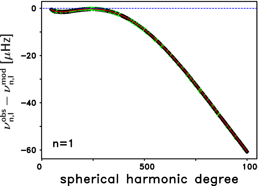
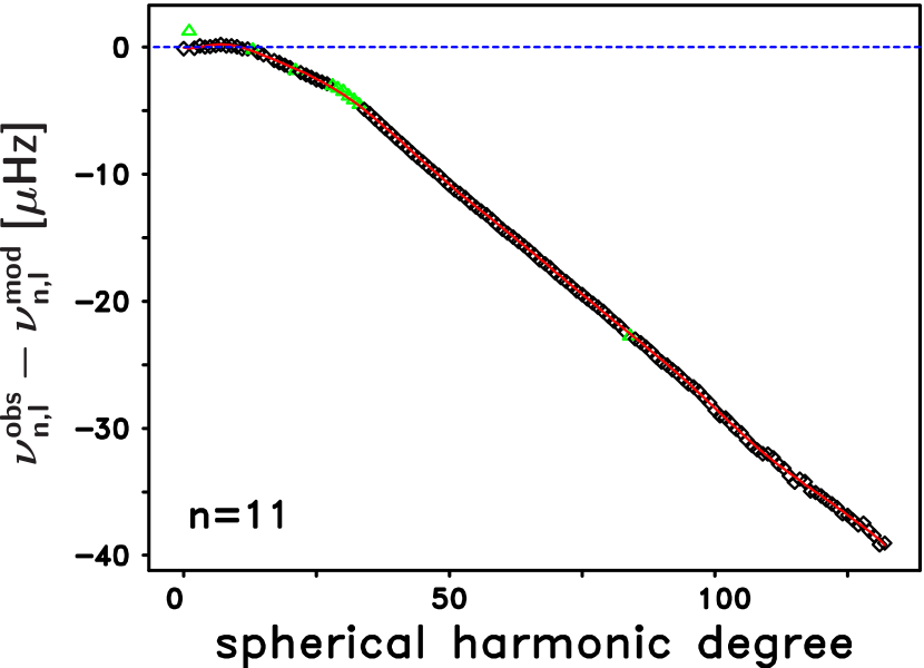
Figure 20: (left) Degree dependence of the differences between the observed frequencies, $\nu_{n,l}^{\rm obs}$, which were computed using Method 2 on the $m$-averaged spectral set $\cal{S}$2010_66a, and the theoretical model frequencies, $\nu_{n,l}^{\rm mod}$, in the sense of Sun minus model, for the $n=1$ ridge. The frequency differences, $\nu_{n,l}^{\rm obs}-\nu_{n,l}^{\rm mod}$, are shown as the black diamonds. The red line is for the Chebyshev polynomial, $\varXi_{\varpi}^{(n)}(l)$, of degree $\varpi=24$ fitted to the frequency differences. The 276 green triangles represent modes flagged as outliers. We note that these frequency differences are the same that were shown as the red curve in the upper-right panel of Figure LABEL:dfm1ms. (right) Same as left panel, but for the $n=11$ ridge. For this ridge the degree of the fitted Chebyshev polynomial, $\varXi_{\varpi}^{(n)}(l)$, is $\varpi=14$, and 10 modes were flagged as outliers. In both panels the dashed blue line is for a frequency difference of zero. Note that the vertical scales are different on the two panels.

7.1.2 Step 2

In the second step of our outlier correction scheme we fit the Chebyshev polynomial, $\varPi_{\pi}^{(n)}(l)$, of degree $\pi$ to the scaled frequency differences, $\delta\nu_{n,l}$, as defined in equation (46), along a ridge of given radial order, $n$, i.e., as a function of degree $l$. We note that the outliers that were identified during step 1 are not used in the fitting of the $\varPi_{\pi}^{(n)}(l)$ polynomials to the scaled frequency differences, $\delta\nu_{n,l}$. Typical examples of fits to the scaled frequency differences are shown here in the left-hand panels of Figure LABEL:fitresvsl for the $n=1$ and $n=11$ ridge, respectively. In both of these left-hand panels of Figure LABEL:fitresvsl the scaled frequency differences, $\delta\nu_{n,l}$, are shown as the black diamonds, and the fitted Chebyshev polynomials, $\varPi_{\pi}^{(n)}(l)$, are shown as the red lines. The degree $\pi$ of the polynomials $\varPi_{\pi}^{(n)}(l)$ depends on the radial order, $n$, and is determined by trial and error. For the ridges in the range $0\leq n\leq 29$ we found values of $\pi$ in the range $1\leq\pi\leq 29$ to be useful. Rather than simply decreasing with increasing $n$, as was the case for $\varpi$, $\pi$ increased from 19 at $n=0$ to 29 at $n=4$ before decreasing to 1 at $n=29$. As with the degree $\varpi$, we have not yet been able to find any approach that would allow us to determine the degree $\pi$ of the polynomials $\varPi_{\pi}^{(n)}(l)$ in an automated manner.

Next in this second step, we determine, for each ridge of radial order, $n$, the fitting residuals, $r_{l}^{(n)}$, of the fit of $\varPi_{\pi}^{(n)}(l)$ to the scaled frequency differences, $\delta\nu_{n,l}$, i.e.,

$$r_{l}^{(n)}=\delta\nu_{n,l}-\varPi_{\pi}^{(n)}(l).$$ (57)

We flag those modes $(n,l)$ as outliers for which the criterion

$$\big{|}r_{l}^{(n)}\big{|}>3\,\,\mbox{std}\big{(}r_{l}^{(n)}\big{)}$$ (58)

is fulfilled. Here, $\mbox{std}\big{(}r_{l}^{(n)}\big{)}$ denotes the standard deviation of the fitting residuals, $r_{l}^{(n)}$, for the ridge of radial order, $n$. For each ridge, $n$, the fit of the polynomial, $\varPi_{\pi}^{(n)}(l)$, to the scaled frequency differences, $\delta\nu_{n,l}$, is repeated until all outliers have been identified by means of the criterion (58).

For further analyses we will need to generate yet another set of emulated frequencies, viz.

$$\nu_{n,l}^{\rm em2}=\nu_{n,l}^{\rm mod}+\frac{1}{q_{n,l}}\left(\frac{\nu_{n,l}^{\rm mod}}{1000}\right)^{3.5}\varPi_{\pi}^{(n)}(l),$$ (59)

which correspond to observed frequencies that would fall exactly onto the curve $\varPi_{\pi}^{(n)}(l)$ that has been fitted to the scaled frequency differences, $\delta\nu_{n,l}$, for the ridge of radial order, $n$. Because the theoretical model frequencies, $\nu_{n,l}^{\rm mod}$, are error-free, the uncertainty of $\nu_{n,l}^{\rm em2}$ is given by

$$\Delta\nu_{n,l}^{\rm em2}=\frac{1}{q_{n,l}}\left(\frac{\nu_{n,l}^{\rm mod}}{1000}\right)^{3.5}\Delta\varPi_{\pi}^{(n)}(l),$$ (60)

with $\Delta\varPi_{\pi}^{(n)}(l)$ being computed from equation (53) with $\varXi_{\varpi}^{(n)}(l)$ being replaced with $\varPi_{\pi}^{(n)}(l)$.

In the fit of the Chebyshev polynomial $\varXi_{\varpi}^{(n)}(l)$ to the unscaled frequency differences, $\Delta\nu_{n,l}$, along a given ridge (cf. Section 7.1.1) as well as in the fit of the Chebyshev polynomial $\varPi_{\pi}^{(n)}(l)$ to the scaled frequency differences, $\delta\nu_{n,l}$, along a given ridge, outliers can only be detected in a reliable manner if the rough trendline of the fitted curve is known as a function of degree a priori. While this basic requirement is fulfilled for the unscaled frequency differences, $\Delta\nu_{n,l}$, because their trendline along a given ridge is only a slowly varying function of degree (cf. Figure 20), it is not fulfilled for the scaled frequency differences, $\delta\nu_{n,l}$, as is demonstrated here in the left-hand panels of Figure LABEL:fitresvsl, for both the $n=1$ and $n=11$ ridge. For the $n=1$ ridge a sharp variation of the trendline with degree is prominent at around $l\approx 60$, as is shown in the upper-left panel of Figure LABEL:fitresvsl, while for the $n=11$ ridge similar sharp variations do occur at about $l\approx 1$ and $l\approx 7$, respectively, as is shown in the lower-left panel of Figure LABEL:fitresvsl. Such sharp variations of the trendline with degree raise the question whether or not they are real features. However, this is important to know because suspicious trends may reflect some essential variations in the solar structure that are not yet known.

In dealing with this issue we found it useful to introduce the emulated scaled frequency differences, $\delta\nu_{n,l}^{\rm em}$, given by

$$\delta\nu_{n,l}^{\rm em}=\left(\nu_{n,l}^{\rm em1}-\nu_{n,l}^{\rm mod}\right)\,q_{n,l}\left(\frac{\nu_{n,l}^{\rm mod}}{1000}\right)^{-3.5},$$ (61)

which differ from the original scaled frequency differences, $\delta\nu_{n,l}$, merely by the replacement of the observed frequencies, $\nu_{n,l}^{\rm obs}$, in equation (46) with the emulated frequencies, $\nu_{n,l}^{\rm em1}$, defined in equation (55). While for some ridges the degree dependence of the trendline of the curve fitted to the original scaled frequencies, $\delta\nu_{n,l}$, cannot be determined in a unique manner mainly because of lurking outliers in the observed frequencies, $\nu_{n,l}^{\rm obs}$, the degree dependence of the trendline of the emulated scaled frequency differences, $\delta\nu_{n,l}^{\rm em}$, is given uniquely. Primarily, this is because the march of the observed frequencies, $\nu_{n,l}^{\rm obs}$, is only a slowly varying function of degree without any sharp variations so that the march of the emulated frequencies, $\nu_{n,l}^{\rm em1}$, with degree is given unambiguously for each ridge by means of a straightforward fit of the Chebyshev polynomial $\varXi_{\varpi}^{(n)}(l)$ to the unscaled frequency differences, $\Delta\nu_{n,l}$ (cf. Section 7.1.1).

On these grounds, the degree dependence of the trendline of the emulated scaled frequency differences, $\delta\nu_{n,l}^{\rm em}$, can be considered, for a given ridge, as a reliable template for the trendline of the curve fitted, as a function of degree, to the original scaled frequency differences, $\delta\nu_{n,l}$. Therefore, by a careful identification of lurking outliers in the observed frequencies, $\nu_{n,l}^{\rm obs}$, as well as a careful selection of the curve (i.e., Chebyshev polynomial $\varPi_{\pi}^{(n)}(l)$ of degree $\pi$) that is fitted to the original scaled frequency differences, $\delta\nu_{n,l}$, along a given ridge, the degree dependence of the trendline of this fitted curve can be made similar to that of the emulated scaled frequency differences, $\delta\nu_{n,l}^{\rm em}$. This is demonstrated here in Figure LABEL:fitresvsl in which we show the degree dependence of the emulated scaled frequency differences, $\delta\nu_{n,l}^{\rm em}$, for the $n=1$ ridge in the upper-right panel, and for the $n=11$ ridge in the lower-right panel, respectively. A close comparison of the left-hand panels and the corresponding right-hand panels of Figure LABEL:fitresvsl clearly indicates that for both the $n=1$ and $n=11$ ridge the trendlines of the curves fitted to the original scaled frequency differences, $\delta\nu_{n,l}$, as a function of degree are in excellent agreement with the corresponding trendlines of the emulated scaled frequency differences, $\delta\nu_{n,l}^{\rm em}$. We therefore can safely presume that the sharp variations with degree to be seen in the degree dependence of the trendlines of the original scaled frequency differences, $\delta\nu_{n,l}$, of both the $n=1$ and $n=11$ ridge are real features. We note that the same analysis is also useful for ridges other than the $n=1$ and $n=11$ ridge.

At the end of the second step of our outlier correction scheme we have the following three diverse sets of frequencies and associated uncertainties at our disposal: the set of observed frequencies $\nu_{n,l}^{\rm obs}$, and the uncertainties $\Delta\nu_{n,l}^{\rm obs}$ thereof, as well as the two sets of emulated frequencies $\nu_{n,l}^{\rm em1}$ and $\nu_{n,l}^{\rm em2}$, respectively, the uncertainties of which are given by $\Delta\nu_{n,l}^{\rm em1}$ and $\Delta\nu_{n,l}^{\rm em2}$, respectively.

7.1.3 Step 3

In the third step of our outlier correction scheme we compute from these three sets of frequencies and associated uncertainties a total of three sets of normalized frequency differences, viz.

$$\Delta\nu_{n,l}^{\rm(1)} =\frac{\nu_{n,l}^{\rm obs}-\nu_{n,l}^{\rm em1}}{\sqrt{\left(\Delta\nu_{n,l}^{\rm obs}\right)^{2}+\left(\Delta\nu_{n,l}^{\rm em1}\right)^{2}}},$$ (62)

$$\Delta\nu_{n,l}^{\rm(2)} =\frac{\nu_{n,l}^{\rm obs}-\nu_{n,l}^{\rm em2}}{\sqrt{\left(\Delta\nu_{n,l}^{\rm obs}\right)^{2}+\left(\Delta\nu_{n,l}^{\rm em2}\right)^{2}}},$$ (63)

$$\Delta\nu_{n,l}^{\rm(3)} =\frac{\nu_{n,l}^{\rm em1}-\nu_{n,l}^{\rm em2}}{\sqrt{\left(\Delta\nu_{n,l}^{\rm em1}\right)^{2}+\left(\Delta\nu_{n,l}^{\rm em2}\right)^{2}}}.$$ (64)

We flag those modes $(n,l)$ as outliers for which at least one of the following criteria is fulfilled:

$$\big{|}\Delta\nu_{n,l}^{\rm(1)}\big{|}>3,\quad\big{|}\Delta\nu_{n,l}^{\rm(2)}\big{|}>3,\quad\big{|}\Delta\nu_{n,l}^{\rm(3)}\big{|}>3.$$ (65)

7.1.4 Step 4

The fourth step of our outlier correction scheme actually consists of two sub-steps. As we already have pointed out in Section 4.2, custom-made seed tables are required as input to the WMLTP method. This is because the fitting profile, as given by equations (26) through (31), depends on the initially not very well known variation of frequency, amplitude, and linewidth with degree, $l$. Therefore, in the first sub-step we update those seed tables by performing an additional iteration of our fixed-point iteration, as described in Section 4.2. In the second sub-step we then refit, by means of the WMLTP method, all of the modes that have been flagged as outliers in steps 1 through 3 of our outlier correction scheme, thereby employing the updated seed tables as input to the WMLTP method to get the refitted frequencies, $\nu_{n,l}^{\rm new}$.

As we have demonstrated in Section 4.2, the fixed-point iteration that is used for the compilation of the custom-made seed tables which are required as input to the WMLTP method converges on a solution rather rapidly. Therefore, it is to be expected that the refitted frequencies, $\nu_{n,l}^{\rm new}$, generated in the second sub-step deviate only slightly from the observed frequencies, $\nu_{n,l}^{\rm obs}$. In fact, in most of our applications we have found that $\nu_{n,l}^{\rm new}\approx\nu_{n,l}^{\rm obs}$. As a result, the fourth step of our outlier correction scheme may be skipped provided the preceding fixed-point iteration has been carried out carefully. In this case, the remaining fifth step of our outlier correction scheme is performed by using $\nu_{n,l}^{\rm new}=\nu_{n,l}^{\rm obs}$.

7.1.5 Step 5

In the final step of our outlier correction scheme, we update all of the modes that have been flagged as being outliers in steps 1 through 3. In some cases we only update the frequencies of those outliers and in other cases we update only the associated uncertainties, and in still other cases we update both the frequencies and their uncertainties at the same time. In addition, as we shall demonstrate in Section 7.1.6, we also encountered a few cases for which neither their frequency nor their uncertainty have been altered by the procedure.

Before making the updates, we first check whether the refitted frequencies $\nu_{n,l}^{\rm new}$, actually constitute an improvement over the originally observed frequencies, $\nu_{n,l}^{\rm obs}$, by calculating the distances $\delta_{\rm old}$ and $\delta_{\rm new}$, respectively, given by

$$\delta_{\rm old}^{2} =\left(\nu_{n,l}^{\rm obs}-\nu_{n,l}^{\rm em1}\right)^{2}+\left(\nu_{n,l}^{\rm obs}-\nu_{n,l}^{\rm em2}\right)^{2},$$ (66)

$$\delta_{\rm new}^{2} =\left(\nu_{n,l}^{\rm new}-\nu_{n,l}^{\rm em1}\right)^{2}+\left(\nu_{n,l}^{\rm new}-\nu_{n,l}^{\rm em2}\right)^{2},$$ (67)

using the emulated frequencies $\nu_{n,l}^{\rm em1}$ and $\nu_{n,l}^{\rm em2}$, respectively, as reference values. If $\delta_{\rm new}^{2}<\delta_{\rm old}^{2}$, we replace the original observed frequency, $\nu_{n,l}^{\rm obs}$, with the refitted frequency, $\nu_{n,l}^{\rm new}$, for that mode, i.e.,

$$\nu_{n,l}^{\rm obs,new}=\nu_{n,l}^{\rm new},$$ (68)

and we set for the associated uncertainty

$$\Delta\nu_{n,l}^{\rm obs,new}=\max\left(\Delta\nu_{n,l}^{\rm obs},\Delta\nu_{n,l}^{\rm new},\Delta\nu_{n,l}^{\rm em1},\Delta\nu_{n,l}^{\rm em2},\left|\nu_{n,l}^{\rm em1}-\nu_{n,l}^{\rm new}\right|/3,\left|\nu_{n,l}^{\rm em2}-\nu_{n,l}^{\rm new}\right|/3\right).$$ (69)

Here, the first four terms on the right-hand side represent all of the various uncertainties available for the mode $(n,l)$ at this point, while the last two terms make sure that the refitted frequency is off by no more than $3\,\sigma$ from the curve that was fit to the unscaled frequency differences, $\Delta\nu_{n,l}$, as well as from the curve that was fit to the scaled frequency differences, $\delta\nu_{n,l}$, in the first and second step of the outlier correction scheme, respectively. If $\delta_{\rm new}^{2}\geq\delta_{\rm old}^{2}$, we do not adjust the original observed frequency, $\nu_{n,l}^{\rm obs}$, but only replace the associated uncertainty with

$$\Delta\nu_{n,l}^{\rm obs,new}=\max\left(\Delta\nu_{n,l}^{\rm obs},\Delta\nu_{n,l}^{\rm em1},\Delta\nu_{n,l}^{\rm em2},\left|\nu_{n,l}^{\rm em1}-\nu_{n,l}^{\rm obs}\right|/3,\left|\nu_{n,l}^{\rm em2}-\nu_{n,l}^{\rm obs}\right|/3\right).$$ (70)

Here, as compared to equation (69) the term $\Delta\nu_{n,l}^{\rm new}$ has been dropped, and in the last two terms $\nu_{n,l}^{\rm new}$ has been replaced with $\nu_{n,l}^{\rm obs}$.

7.1.6 Summary of outlying cases

By means of our outlier correction procedure we detected a total of 2,483 outliers in the entire set of 6,366 modes that we originally inverted (i.e., a total of 39 % of the fitted modes were flagged as being outlying cases). For 1,156 of them we found improved frequencies, $\nu_{n,l}^{\rm new}$, by refitting the corresponding modes, and by then replacing the original observed frequencies, $\nu_{n,l}^{\rm obs}$, with $\nu_{n,l}^{\rm new}$ whenever $\delta_{\rm new}^{2}<\delta_{\rm old}^{2}$, while for the remaining 1,327 outliers it turned out that the corresponding refitted frequencies were not an improvement over the original observed frequencies, $\nu_{n,l}^{\rm obs}$, because of $\delta_{\rm new}^{2}\geq\delta_{\rm old}^{2}$, and hence we left the original observed frequencies unchanged.

In Figure 21 we illustrate the location of the outliers in the $l$-$\nu$ plane that were detected by means of our outlier correction procedure. The 1,156 outliers for which we were able to compute an improved refitted frequency are shown as the red diamonds, while the 1,327 outliers for which our refitted frequency was not an improvement over our original, observed frequency, are shown as the green diamonds. When we examined the spherical harmonic degree distribution of both sets of outliers, we found that both sets were primarily located at low and moderate degrees rather than at high degrees. In fact, we found that 75 % of the 2,483 outliers were located at or below $l=350$.

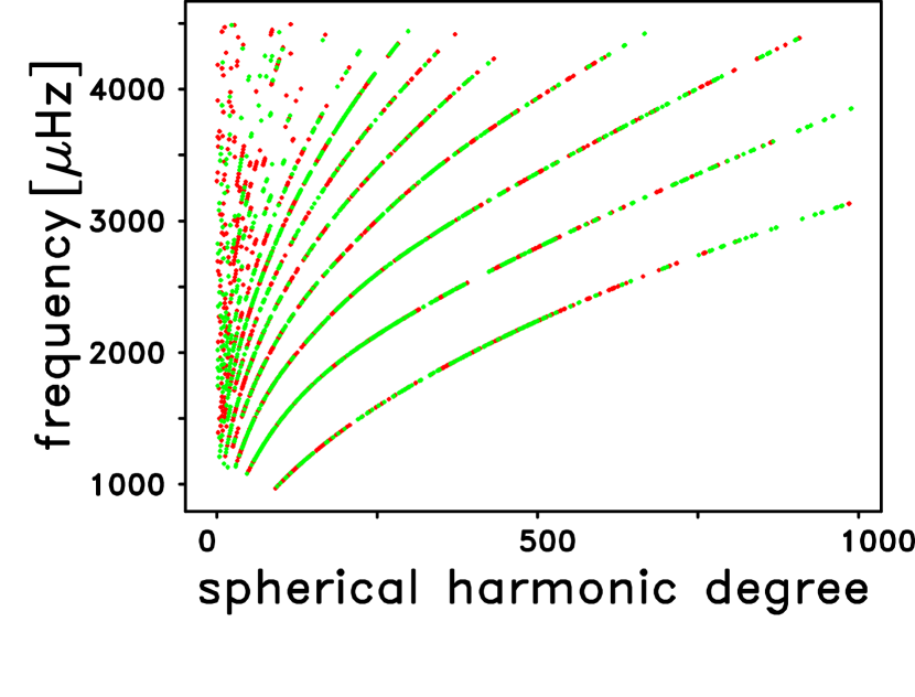
Figure 21: Location of the outlying cases in the $l$-$\nu$ plane that have been detected by means of the outlier correction scheme as described in Section 7.1. The red diamonds are for the 870 outliers for which both the frequencies and their uncertainties were adjusted and for the 286 additional outliers for which only the frequencies were adjusted. The green diamonds are for the 1,129 outliers for which only the frequency uncertainties were adjusted and for the remaining 198 cases for which neither the frequencies nor their uncertainties needed to be adjusted.

Of the 1,156 cases for which we were able to compute an improved refitted frequency, we found far more cases (e.g., 1,031) for which the refitted frequency was lower than the original frequency. That left only 125 cases for which the refitted frequency was higher than was the original frequency. Furthermore, for only 143 of the 1,156 cases were we able to find a normalized frequency adjustment that was greater than $3\,\sigma$ in absolute magnitude.

By means of either equation (69) or (70) we tried to find improved estimates for the frequency uncertainties of the 2,483 outliers. Such adjustment of the frequency uncertainties is in a sense equivalent to the allowance of systematic errors in the observed frequencies, $\nu_{n,l}^{\rm obs}$, and $\nu_{n,l}^{\rm obs,new}$, respectively. A summary of the statistics that resulted when we carefully evaluated the frequency uncertainties of all 2,483 outliers using equations (69) and (70) is given in Table 7. In the first column of Table 7 the eight terms are listed that could trigger the modification of the frequency uncertainty of an outlying case according to either equation (69) or (70). In the second column of Table 7 we list the number of cases for which one of the terms included in the right-hand side of equation (69) triggered the adjustment of the frequency uncertainty. Interestingly, we found that $\Delta\nu_{n,l}^{\rm obs,new}=\Delta\nu_{n,l}^{\rm obs}$ for 286 cases, as shown in the first row of column 2 in Table 7, and therefore we did not alter the original frequency uncertainty, $\Delta\nu_{n,l}^{\rm obs}$, of those cases. For the remaining 870 cases we increased the original frequency uncertainty because one of the terms listed below $\Delta\nu_{n,l}^{\rm obs}$ in the first column of Table 7 turned out to be larger in magnitude than $\Delta\nu_{n,l}^{\rm obs}$. In the third column of Table 7 we list the number of cases that we evaluated using equation (70). For 1,129 of these 1,327 cases, we ended up increasing the original frequency uncertainties; however, for the remaining 198 cases the original frequency uncertainty was large enough that it did not need to be replaced with one of the other terms in equation (70). In summary, considering all of the 2,483 outliers we found an average ratio of the final and original uncertainties of $1.974\pm 1.237$. When we included only the 1,999 cases for which the frequency uncertainty actually increased in the computation of the average ratio of the new to the original uncertainties, we found that the average ratio was increased slightly to $2.210\pm 1.271$.

The 198 outliers listed at the top of the third column in Table 7 are those cases for which neither the frequencies nor the frequency uncertainties needed to be changed. Therefore, the question arises as to why those 198 cases were flagged as being outliers in the first case. This can happen because we are invoking two criteria for the identification of outliers which do not depend in any way upon the frequency uncertainty, $\Delta\nu_{n,l}^{\rm obs}$. These criteria are given in equation (58) and in the third branch of equation (65), respectively. As a result, if a mode is initially flagged as being an outlier by one of those two criteria, but later its refitted frequency is not found to be an improvement over the original frequency of that mode, $\nu_{n,l}^{\rm obs}$, and also if the original frequency uncertainty of that mode, $\Delta\nu_{n,l}^{\rm obs}$, is large enough in magnitude that equation (70) sets $\Delta\nu_{n,l}^{\rm obs,new}=\Delta\nu_{n,l}^{\rm obs}$, this mode ends up with both its original frequency and its original uncertainty intact. We note, however, that such a mode is not expected to hamper the convergence of the inversion code because of its exceptionally large frequency uncertainty, $\Delta\nu_{n,l}^{\rm obs}$, that has been returned by the WMLTP code for this mode.

In spite of the above discussion about the number of outliers that our procedure identified, we wish to stress that, in the majority of the 6,366 original fits for which $\nu\leq 4500\,\,\mu$Hz, we did not find it necessary to alter our original fitted frequencies and/or uncertainties thereof at all. We illustrate this important point further in Table 8 in which we have summarized the various outcomes of our five-step procedure. In the second row of Table 8 we note that we did not have to alter the frequencies of 5,210, or 81.8 %, of our 6,366 original fits. This overwhelming majority of our cases was comprised of the 3,883 cases that were never identified as being outliers by our procedure, the 1,129 cases for which only the frequency uncertainties needed to be altered, and the 198 cases for which neither the frequencies nor their uncertainties needed to be adjusted. Also, in the third row of Table 8 we note that a total of 4,367, or 68.6 %, of our original cases did not need to have their uncertainties altered. This number was comprised of the 3,883 cases that were never identified as being outliers, the 286 cases for which only the frequencies needed to be altered, and the 198 cases for which neither the frequencies nor the uncertainties needed to be altered. In the remaining rows of Table 8 we summarize the 2,483 outlying cases and their outcomes that resulted from the various steps of our procedure in diminishing order as percentages of our total of 6,366 original cases.

While Table 8 shows that our outlier identification and correction procedure ended up requiring an increase in a total of 1,999 of the original frequency uncertainties, we note that these increases were found to be needed because the original uncertainties that the WMLTP code computed were too small. In this regard, it is important to note that the formal uncertainties delivered by the WMLTP code only represent the statistical errors which are not corrected for any systematic effects. Therefore, our outlier correction scheme is useful not only for detecting systematic errors in the sets of fitted frequencies but also for detecting frequency uncertainties that are unduly small. We finally note that it is both the correction of the fitted frequencies for systematic errors as well as the adequate adjustment of the frequency uncertainties by means of our outlier correction scheme that finally allowed the inversion shown in Figure 22 to converge properly on a solution.

7.2 Inversion results

Accurate measurements of the high-degree solar oscillation modes are particularly important for helioseismic diagnostics of the near-surface layers of the Sun. These layers are believed to play a critical role in the formation of the magnetic network, sunspots and active regions, and thus are a key to understanding the mechanisms of solar activity and variability. To illustrate the potential of the new method of measurements of the high-degree mode frequencies we performed a standard inversion procedure for the solar sound-speed profile, which is based on the mode sensitivity kernels derived from the variational principle, and the OLA inversion method. The sensitivity kernels are calculated from the adiabatic eigenfunctions, and the surface non-adiabatic effects are removed by assuming that these can be described as a function of frequency, weighted with the mode inertia (cf. equation (46)). The inversion method provides locally averaged estimates of the sound-speed variations at various target positions along the solar radius. The central locations and characteristic width (“spread”) of the averaging kernels of these estimates provide a quantitative measure of the resolving power of the observed frequency set. The mathematical details of the inversion procedure are described by Kosovichev (1999).

The inversion results illustrated in Figure 22 show the relative deviations of the squared sound speed in the Sun from the standard solar Model S (Christensen-Dalsgaard et al., 1996). The results reproduce a well-known peak at the base of the convection zone, which is associated with the tachocline – a narrow area of the strong rotational shear at the bottom of the convection zone (Kosovichev, 1996a; Elliott & Gough, 1999). In the lower part of the convection zone, the sound-speed deviation is almost zero due to the adiabatic stratification of the radial structure. The sound-speed profile gradually decreases relative to the model in the bulk of the convection zone, which may indicate a deviation from the adiabatic stratification of the model (prescribed by the mixing-length theory of convection), and then shows a sharp decrease in the upper 5 % of the solar radius ($\sim 35$ Mm). Such decrease in the sound speed was previously detected by inversions, however, its structure was not resolved. The new results show that the structure of the near-surface layer is now well-resolved. The substantial deviation from the model coincides with the subsurface rotational shear layer (called “leptocline” by Godier & Rozelot, 2001), and indicates that the structure of the solar convection zone and the heat transport properties may be significantly different from the predictions of the mixing-length theory. Of course, this result is only a starting point of systematic investigations of the global structure and dynamics of this layer, and also of the variations with the solar cycle.

Figure 22: The relative squared sound-speed deviations from the Standard Solar Model S of Christensen-Dalsgaard et al. (1996) as a function of fractional radius that we obtained by a structural inversion of the 6,366 frequencies and their uncertainties that resulted from the application of the outlier correction procedure to our original frequency table that has been computed using Method 2 on the $m$-averaged spectral set $\cal{S}$2010_66a, and covered the frequency range of 969 to $\,4500\,\,\mu$Hz. The horizontal bars represent the width (“spread”) of the localized averaging kernels, providing a characteristic of the spatial resolution; the vertical bars are the formal error estimates.

8 Concluding remarks

Global helioseismology has proven to be an extremely powerful tool for the investigation of the internal structure and dynamical motions of the Sun and, thus, should not be abandoned in favor of local helioseismology alone. Numerical inversions of low- and medium-degree solar oscillation frequencies have confirmed that the solar structure is in remarkably good agreement with predictions of the standard solar model. However, global helioseismic studies have not yet provided reliable information about the very interesting near-surface region of the Sun because high-degree modes were not measured accurately enough due to serious problems in the understanding of the structure of a ridge of oscillatory power and various distortion effects of the measuring device.

In order to provide a more-accurate characterization of the high-degree ridges of power, we have presented in this paper a sophisticated mathematical method for the fitting of $m$-averaged power spectra which employs a theoretical profile that contains multiple peaks which represent each mode of interest and also its surrounding temporal and spatial sidelobes. This method includes both spatial leakage matrices which weight each of the spatial sidelobes differently according to the details of the instrument which provided the data from which the power spectra were created, and it also includes the temporal window function of each observational time series to allow for the data gaps that are usually present in the observations.

In Section 2 above, we outlined several different approaches to the calculation of $m$-averaged spectra, and we also described the need for the correction of the frequency splitting coefficients which are used in the generation of such spectra for the effects of modal distortions that are introduced by solar latitudinal differential rotation. In Section 3 we presented mathematical details of the computation of the spatial leakage matrices which are required for the accurate fitting of both isolated modal peaks and ridges of power, and we presented the mathematical details of the method by which such leakage matrices are corrected for the effects of differential rotation. In Section 4 we presented the mathematical details of this new method, which we have named the WMLTP method, and which we have also referred to in the text as our Method 2.

In Section 5 we presented the results of a series of studies of the sensitivity of the fitted frequencies that this method produces to various details of the method of generating the $m$-averaged power spectra and of the approximation that is made to the shape of the various leakage matrix peaks. In Section 5.1.1 we showed that the weighting of the individual tesseral and sectoral power spectra at each degree prior to the computation of the $m$-averaged spectrum had only a very minor influence on the resulting frequencies. On the other hand, in Section 5.1.2, we showed that the use of frequency-splitting coefficients that were computed in a non-$n$-averaged manner and which were also corrected for the distorting effects of differential latitudinal rotation definitely did result in substantial changes to the fitted frequencies. In Section 5.1.3 we showed that the majority of these systematic frequency changes were due to the use of such non-$n$-averaged frequency-splitting coefficients in place of coefficients that were computed in an $n$-averaged manner. That is, we demonstrated the importance of using a narrow frequency range that was centered on each individual ridge when cross-correlating the non-zonal power spectra with the zonal spectrum at each degree. In Section 5.2 we showed that an increase of 18 % in the width of the Gaussian function that we employ in Method 2 as an approximation of the peaks in the effective leakage matrices did not result in any systematic frequency changes.

In Section 6 we demonstrated the substantial improvements that the WMLTP method makes in the frequencies, linewidths, amplitudes, and in the uncertainties of all of these quantities in comparison with the same quantities computed using our earlier Method 1, which only employed a single Lorentizan profile in place of the more complicated multiple-peak profile of Method 2. In particular, we have pointed out that the use of a multiple-peak profile in the WMLTP method reduces the formal frequency uncertainties by a factor of $15.2\pm 0.3$ on average, and it also reduced the formal linewidth uncertainties by a factor of $29.8\pm 0.9$ on average. We have also demonstrated that the frequencies, linewidths, and amplitudes that we computed using the multiple-peak profile do not exhibit any sharp discontinuities along the various ridges as did the same quantities that were obtained using the single-peak profile. These discontinuities occurred where the individual peaks became blended into broad ridges of power at the higher degrees. We have also compared the relative smoothness of both the frequencies and linewidths which were computed with the WMLTP method from various sets of power spectra that were obtained with the MDI instrument. We have also displayed the sets of 12,359 frequencies, linewidths, amplitudes, asymmetries, and power levels that we generated by applying the WMLTP method to the 66-day long 2010 MDI Dynamics Run power spectra.

In Section 7.1 we presented the details of a new procedure that we developed to improve both the numerical stability and reliability of the structural inversion that we presented in Section 7.2 and of similar structural inversions that we expect to compute with similar Method 2 frequency tables in the future. This procedure both identifies and corrects outliers in both the frequencies and their associated uncertainties. We applied it to the subset of 6,366 Method 2 frequencies that we had originally inverted and we obtained a much smoother inverted sound speed deviation profile in the process.

In conclusion, we have shown that the development of the WMLTP method of power spectral fitting provides a powerful new tool for the provision of accurate and reliable estimation of low-, intermediate, and high-degree mode parameters. We demonstrated this claim impressively in Section 7.2 with the presentation of a new structural inversion corresponding to the beginning of Solar Cycle 24 that we computed using our cleaned table of MDI 2010 Dynamics Run frequencies. This new inversion resolves for the first time the seismic properties of the upper convective boundary layer, and shows a substantial and surprisingly sharp deviation from the adiabatic sound-speed profile of the Standard Solar Model S of Christensen-Dalsgaard et al. (1996), which is likely due to the near-surface turbulence effects. Moreover, this is also evidence that the predictions of the mixing-length theory may be significantly different from both the actual structure of the convection zone and the heat transport properties in the subsurface layers of the Sun. By comparing upcoming structural inversions similar to that presented here in Section 7.2 with realistic 3D MHD numerical simulations of the upper solar convection zone and the subsurface shear layer we hope to make significant progress in the understanding of the structure and dynamics of the outer layers of the Sun. In this regard, we note that the detailed measurements of the linewidths of the $f$- and $p$-modes could also provide useful constraints on the properties of near-surface convection (cf. Christensen-Dalsgaard et al., 1989; Rabello-Soares et al., 1999).

Because for degrees $l\gg 1$ $m$-averaging of the originally generated zonal, sectoral, and tesseral power spectra significantly improves the signal-to-noise ratio, the WMLTP method is particularly well suited for the fitting of $m$-averaged power spectra derived from time series as short as three days, say. This facilitates the detailed investigation of temporal frequency shifts with the phase of the solar activity cycle (see, e.g., Ronan et al., 1994; Jefferies, 1998; Rhodes et al., 2002, 2003; Rose et al., 2003; Rabello-Soares et al., 2008b; Tripathy et al., 2010; Jain et al., 2011; Rhodes et al., 2011). On the other hand, the generation of $m$-averaged power spectra requires knowledge of suitable frequency splitting coefficients (cf. Sect. 2.2). Therefore, as we mentioned in Section 2.3, we have also begun to develop our MPTS fitting method which operates directly upon all $2l+1$ un-averaged power spectra for each degree. The MPTS method allows us to determine all $2l+1$ sets of modal parameters of a given $(n,l)$ multiplet. Once we have determined all $2l+1$ of the frequencies of that multiplet, we can then compute both the average frequency and the frequency-splitting coefficients for that multiplet. In essence, the MPTS method will allow us to generate sets of non-$n$-averaged frequency splitting coefficients without recourse to the cross-correlation method that we described in Section 2.2. Details of the MPTS method will be given in the upcoming second paper of our series of three papers.

Unfortunately, as we mentioned earlier the MPTS method cannot be applied to power spectra that are computed from time series that are as short as three days in duration, nor can it fit peaks having frequencies greater than about $5000\,\,\mu$Hz because of the low signal-to-noise ratios of the underlying power spectra. As a result of these two limitations, both the WMLTP and MPTS fitting methods are complementary to each other. Hence, we hope that, once we have been able to bring the current version of the MPTS code up to the level of the rev6 version of the WMLTP code, the parallel application of both fitting methods will lead to new information concerning temporal variations in the Sun’s sub-surface structure and dynamics.

Appendix A The single-peak, averaged-spectrum method

The Single-Peak, Averaged-Spectrum, or SPAS, Method, which is also referred to as Method 1, was our initial, first-generation fitting method. It was developed in the late-1980s through the mid-1990s in order to fit the peaks in the MDI power spectra that were generated as part of that experiment’s Structure Program (Scherrer et al., 1995). This work led to the publication of a set of tables of $f$- and $p$-mode frequencies and their associated errors which has become a major reference in the helioseismic literature for the MDI Medium-$l$ Program (Rhodes et al., 1997). We also have applied Method 1 to the analysis of power spectra which were derived from MDI’s Full-Disk (FD) Dynamics Program (Scherrer et al., 1995). This led to the publication of the first frequencies to be computed for the high-degree modes from the MDI FD spectra (Rhodes et al., 1998a, b).

In Method 1 a single, symmetric Lorentzian profile plus a linear background term is used as the model profile to represent an oscillation peak, i.e.,

$$M(\nu,\mbox{\boldmath$p$}) = \frac{A}{1+x^{2}}+a+b\,\nu,\,\,\,x=\frac{2\,(\nu-\nu_{0})}{w},$$ (A1)

$$p = (A,\nu_{0},w,a,b)^{\mbox{\footnotesize T}},$$ (A2)

with $\nu$ being frequency. The five fit parameters are collected in the vector $p$, and include, respectively, the mode amplitude $A$, the mode frequency $\nu_{0}$, the mode linewidth $w$, and the background noise parameters $a$ and $b$. The vector $p$ is determined by fitting the model profile (A1) in the least-squares sense to the $m$-averaged spectrum in a fitting range centered about the peak of interest that is selected by using the heuristic approach as described below. The resulting unconstrained least-squares problem is solved by using the FORTRAN routine lmder1 from the MINPACK project (Moré et al., 1980). This routine is designed to minimize the sum of squares of $\lambda_{1}$ nonlinear functions in $\lambda_{2}$ variables ($\lambda_{2}\leq\lambda_{1}$) by a modification of the Levenberg-Marquardt algorithm (Levenberg, 1944; Marquardt, 1963).

The variance of the $i$th fit parameter $p_{i}\in\mbox{\boldmath$p$}$ is calculated from

$$\mbox{var}\,p_{i}=\frac{2\,S}{\lambda_{1}-\lambda_{2}}\,H^{-1}_{ii},$$ (A3)

where $\lambda_{1}$ is the number of data points (frequency bins), $\lambda_{2}$ is the number of fit parameters, $H^{-1}_{ii}$ is the $i$th diagonal element of the inverse of the Hessian matrix $H$, and $S$ is the sum of squares of the fit residuals (NAG Fortran Library, Mark 23, 2011). Both $H$ and $S$ are calculated at the solution of the least-squares problem. In the neighborhood of the solution the Hessian matrix can be adequately approximated by

$$H=2\,J^{T}J,$$ (A4)

with $J$ being the Jacobian matrix, thereby avoiding the need to compute or approximate second derivatives of the objective function (Gill et al., 1981). The $100\,(1-\gamma)$ percent confidence interval on the $i$th fit parameter $p_{i}$ is given by

$$p_{i}\pm\sqrt{\mbox{var}\,p_{i}}\,\,t_{1-\gamma/2,\lambda_{1}-\lambda_{2}},$$ (A5)

where $t_{1-\gamma/2,\lambda_{1}-\lambda_{2}}$ is the $100\,(1-\gamma/2)$ percentage point of Student’s t-distribution with $\lambda_{1}-\lambda_{2}$ degrees of freedom (Wolberg, 1967; NAG Fortran Library, Mark 23, 2011). For $1\,\sigma$ confidence intervals $\gamma=0.31731$, and for $\lambda_{1}-\lambda_{2}\gg 1$ we have $t_{1-\gamma/2,\lambda_{1}-\lambda_{2}}\approx 1$.

We have implemented into Method 1 an option which allows to use either a narrow fitting range or else a wide fitting range. We switch between the narrow and the wide fitting range based upon the ratio, $r$, between the linewidth and the frequency change with respect to degree, namely

$$r=\frac{w}{\Delta\nu/\Delta l}.$$ (A6)

We estimate this ratio using linewidths and frequencies from seed tables that have been derived from previously computed modal parameters. We use the narrow fitting range when $r<r_{\rm crit}$ and the wide fitting range for $r\geq r_{\rm crit}$, namely when the modes are well separated, or not, from the spatial leaks of nearby degrees. Because there is no sharp transition between modes and ridges of power, the choice of $r_{\rm crit}$ is somewhat arbitrary. By visual inspection of the fits obtained with Method 1 we found the values

$$r_{\rm crit}=\left\{\begin{array}[]{l@{\quad}l}0.65&\mbox{for~{}~{}$n=0$,}\\[2.84526pt] 0.80&\mbox{for~{}~{}$n>0$,}\end{array}\right.$$ (A7)

to be useful. For the $n=0$ ridge we had to select a separate value of $r_{\rm crit}$ because for this ridge individual modal peaks blend into ridges of power for smaller ratios, $r$, than for the other ridges. The values of $r_{\rm crit}$ given in equation (A7) correspond to $l\approx 278$ for $n=0$, $l\approx 208$ for $n=1$, and $l\approx 15$ for $n=29$.

In the left panels of Figure LABEL:F2 we show typical fits obtained with Method 1 when applied to the $m$-averaged spectral set $\cal{S}$2010_66a. The fits obtained by using a narrow fitting range are shown as the green lines, while the blue lines are for fits that employed the wide fitting range. We note that the use of both the narrow and wide fitting ranges for $(n,l)=(2,70)$ and $(2,200)$ in the top-left and middle-left panel of this Figure required the cancellation of the criterion (A7), which would have enforced the use of the narrow fitting range for $(2,70)$ and the use of the wide fitting range for $(2,200)$. From the colored tick marks in these two panels it becomes evident that the frequencies determined with the wide fitting range differ significantly from those obtained with the narrow fitting range. This is also demonstrated in Table 6. We stress that while this disagreement is obvious in the cases of those modes for which the peaks are well resolved, the very same problems are occurring in the cases of broad ridges of power even though the observed peaks do not show evidence of the individual spatial leaks as is shown here in the bottom-left panel of Figure LABEL:F2.

This so-called “frequency pulling” of the measured ridge-fit frequencies away from the true solar frequencies was first addressed by Libbrecht & Kaufman (1988), and is mainly caused by the asymmetry of the power distribution of the spatial leaks with respect to the target mode frequency (Korzennik et al., 2004). We first tried to resolve this problem by developing a frequency-correction scheme in which we fitted those modes for which the target peak and the spatial leaks are well separated with both the narrow fitting range and the wide fitting range in Method 1 as is shown here in the top-left and the middle-left panel of Figure LABEL:F2. In order to be able to do so we had to override criterion (A7), of course. By means of a multiple linear regression we then tried to correct the frequencies obtained with the wide fitting range for the effects of mode blending using the differences between the narrow- and wide-fit frequencies. However, we eventually had to abandon this approach because the range of degrees for which the multiple linear regression model can be directly computed, namely, those degrees for which the modal peaks are not blended into ridges of power, is not large enough to allow the regression model to be safely extrapolated up to degrees of 1000 and higher where it is needed (Rhodes et al., 2001).

Appendix B Estimates of smoothness of fitted parameters

On physical grounds it can be assumed that any modal parameter, e.g., frequency or linewidth, is a smooth function of spherical harmonic degree $l$ along a ridge of radial order $n$. We suggest to measure the smoothness of any modal parameter along a ridge by the so-called normalized point-to-point scatter, $\varSigma(\upsilon)$, defined by

$$\varSigma^{2}(\upsilon)=\frac{1}{2\,(l_{\rm max}-l_{\rm min})}\sum\limits_{i=l_{\rm min}}^{l_{\rm max}-1}(\upsilon_{i+1}-\upsilon_{i})^{2},$$ (B1)

where $\upsilon$ is the variable/parameter whose smoothness is estimated, and $l_{\rm min}$ and $l_{\rm max}$ are, respectively, the minimum and maximum degree $l$ of the portion of interest of the ridge. Because $\varSigma(\upsilon)$ is rather sensitive to missing cases $\upsilon_{i}$ we recommend that any gaps that might exist in the range from $l_{\rm min}$ to $l_{\rm max}$ are filled by interpolation. We note that the value of $\varSigma(\upsilon)$ is biased towards any slope of the variable $\upsilon$ that might exist in the range from $l_{\rm min}$ to $l_{\rm max}$ because such slope causes the differences $\upsilon_{i+1}-\upsilon_{i}$ in equation (B1) to be systematically different from zero. In general, however, this bias is concealed by the scatter of the differences $\upsilon_{i+1}-\upsilon_{i}$ due to noise.

Table 1: Epochs of observing runs used in this work.

run	starting and end date	duration	Duration	gap-filled
		(days)	(60-sec samples)	duty cycle
$\cal{R}$1996_61	May 24 - Jul 23, 1996	60.75	87,480	97.30 %
$\cal{R}$2001_90	Feb 24 - May 28, 2001	90	129,600	97.02 %
$\cal{R}$2010_66	May 7 - Jul 11, 2010	66	95,040	93.87 %
$\cal{R}$2010_03	May 7 - May 9, 2010	3	4,320	85.52 %

Note. — Column 1 lists the naming convention we assigned to each observing run. Columns 2 through 5 contain the starting and ending dates, the durations in days, the durations in 60-second samples, and the gap-filled duty cycles of the four runs, respectively. Each observing run was obtained as part of the MDI Full-Disk Program (Scherrer et al., 1995).

Table 2: Sets of $m$-averaged spectra used in this work.

observing	$m$-averaged	$m$-averaging	frequency splitting
run	spectral set		coefficients
$\cal{R}$1996_61	$\cal{S}$1996_61	unweighted	corrected, $n$-averaged
$\cal{R}$2001_90	$\cal{S}$2001_90	unweighted	corrected, $n$-averaged
$\cal{R}$2010_66	$\cal{S}$2010_66a	unweighted	corrected, $n$-averaged
$\cal{R}$2010_66	$\cal{S}$2010_66b	weighted	corrected, $n$-averaged
$\cal{R}$2010_66	$\cal{S}$2010_66c	weighted	raw, non-$n$-averaged
$\cal{R}$2010_66	$\cal{S}$2010_66d	weighted	corrected, non-$n$-averaged
$\cal{R}$2010_03	$\cal{S}$2010_03	unweighted	corrected, $n$-averaged

Note. — Column 1 lists the observing run using the naming convention introduced in Table 1. Column 2 lists the naming convention we assigned to each $m$-averaged spectral set that we computed from the un-averaged power spectra obtained from the observing run listed in the same row of column 1. Column 3 indicates whether the averaged spectra were computed using the weights described in Section 2.2 or were computed in an unweighted manner. Column 4 describes the type of frequency splitting coefficients that were employed in the averaging step.

Table 3: Performance of the fixed-point iteration for the construction of accurate seed tables using the example of the frequency, $\nu$.

difference	$n_{c}$	$n_{\rm out}$	avg	std
$\displaystyle\left(\frac{\Delta\nu}{\Delta l}\right)_{n,l}^{\rm(seed,2)}-\left(\frac{\Delta\nu}{\Delta l}\right)_{n,l}^{\rm(seed,1)}$	12,408	22	$-2.456\cdot 10^{-3}$	$1.236\cdot 10^{-1}$
$\displaystyle\left(\frac{\Delta\nu}{\Delta l}\right)_{n,l}^{\rm(seed,3)}-\left(\frac{\Delta\nu}{\Delta l}\right)_{n,l}^{\rm(seed,2)}$	12,417	21	$+4.640\cdot 10^{-4}$	$8.988\cdot 10^{-2}$
$\displaystyle\frac{\nu_{n,l}^{\rm(fit,2)}-\nu_{n,l}^{\rm(fit,1)}}{\max(\Delta\nu_{n,l}^{\rm(fit,1)},\Delta\nu_{n,l}^{\rm(fit,2)})}$	12,417	13	$-1.993\cdot 10^{-1}$	$1.819\cdot 10^{0}$
$\displaystyle\frac{\nu_{n,l}^{\rm(fit,3)}-\nu_{n,l}^{\rm(fit,2)}}{\max(\Delta\nu_{n,l}^{\rm(fit,2)},\Delta\nu_{n,l}^{\rm(fit,3)})}$	12,353	85	$-8.816\cdot 10^{-7}$	$1.129\cdot 10^{-4}$

Note. — Columns 2 through 5 contain the number of cases considered, $n_{c}$, the number of rejected outliers, $n_{\rm out}$, the average, avg, and the standard deviation, std, of the cases listed in column 1. The values of the frequency derivative, $\left(\Delta\nu/\Delta l\right)_{n,l}^{\rm(seed,k)}$, $k=1,2,3$, were input as seeds into the WMLTP code to generate the fitted frequencies, $\nu_{n,l}^{\rm(fit,k)}$, $k=1,2,3$. The differences of the frequency derivatives, $\left(\Delta\nu/\Delta l\right)_{n,l}^{\rm(seed,k)}$, that are listed in rows 1 and 2, respectively, are unscaled, while the differences of the fitted frequencies, $\nu_{n,l}^{\rm(fit,k)}$, that are listed in rows 3 and 4, respectively, are scaled by the maximum of the uncertainties of the frequencies that are subtracted.

Table 4: Fitted parameters invoked in the individual passes used for determining the fitting vector $p$.

	fitted parameters					fitted parameters
	main peak & background					$n$-leaks
pass						$i=1,\ldots,N$
# 1	$A_{n,l}$				$a$, $b$, $c$
# 2		$\nu_{n,l}$	$w_{n,l}$
# 3	$A_{n,l}$	$\nu_{n,l}$	$w_{n,l}$		$a$, $b$, $c$
# 4	$A_{n,l}$				$a$, $b$, $c$	$A_{i}$
# 5		$\nu_{n,l}$			$a$, $b$, $c$		$\nu_{i}$
# 6			$w_{n,l}$		$a$, $b$, $c$			$w_{i}$
# 7	$A_{n,l}$	$\nu_{n,l}$	$w_{n,l}$		$a$, $b$, $c$	$A_{i}$	$\nu_{i}$	$w_{i}$
# 8	$A_{n,l}$	$\nu_{n,l}$	$w_{n,l}$		$a$, $b$, $c$	$A_{i}$	$\nu_{i}$	$w_{i}$
# 9	$A_{n,l}$	$\nu_{n,l}$	$w_{n,l}$		$a$, $b$, $c$	$A_{i}$	$\nu_{i}$	$w_{i}$
# 10	$A_{n,l}$	$\nu_{n,l}$	$w_{n,l}$		$a$, $b$, $c$	$A_{i}$	$\nu_{i}$	$w_{i}$
# 11				$B_{n,l}$					$B_{i}$
# 12	$A_{n,l}$	$\nu_{n,l}$	$w_{n,l}$		$a$, $b$, $c$	$A_{i}$	$\nu_{i}$	$w_{i}$
# 13	$A_{n,l}$	$\nu_{n,l}$	$w_{n,l}$	$B_{n,l}$	$a$, $b$, $c$	$A_{i}$	$\nu_{i}$	$w_{i}$	$B_{i}$

Note. — The value of a parameter that is not invoked in a specific pass is set to either its initial guess or else to its value as determined in a previous pass. For the initial guess of the line asymmetry parameter we use $B_{n,l}=0$ and $B_{i}=0$, $i=1,\ldots,N$. The initial guesses of the remaining fit parameters are taken from a seed table. If the symmetrical profile is used $B_{n,l}$ and $B_{i}$, $i=1,\ldots,N$ are kept fixed to zero in passes # 11 and # 13. To increase the numerical stability of the WMLTP code rather tight constraints are applied to the fitted parameters in passes # 1 through # 7. The rationale for passes # 8 through passes # 10 is to gradually relax these constraints as much as possible.

Table 5: Statistical analysis of the magnitude of raw and scaled frequency differences obtained from four comparisons C1 through C4 in the study of the sensitivity of Method 2 to the details of the $m$-averaging procedure and the effective leakage matrix, respectively.

			$\nu<7000\,\,\mu$Hz				$\nu<4500\,\,\mu$Hz
			$\mbox{avg}\pm\mbox{std}$	ste	$n_{\rm tot}$	$n_{\rm out}$	$\mbox{avg}\pm\mbox{std}$	ste	$n_{\rm tot}$	$n_{\rm out}$
C1:	1	$|\Delta\nu|$	$0.265\pm 0.514$	0.005	12,353	55	$0.044\pm 0.137$	0.002	6,421	4
	2	$|\Delta\nu/\sigma_{\Delta\nu}|$	$1.062\pm 1.075$	0.010	12,353	3	$1.076\pm 1.177$	0.015	6,421	3
C2:	3	$|\Delta\nu|$	$0.403\pm 0.484$	0.004	12,158	24	$0.278\pm 0.301$	0.004	6,235	0
	4	$|\Delta\nu/\sigma_{\Delta\nu}|$	$4.858\pm 6.398$	0.058	12,158	79	$7.786\pm 7.689$	0.098	6,235	79
C3:	5	$|\Delta\nu|$	$0.328\pm 0.403$	0.004	12,159	38	$0.302\pm 0.331$	0.004	6,236	0
	6	$|\Delta\nu/\sigma_{\Delta\nu}|$	$5.786\pm 8.403$	0.076	12,159	5	$10.225\pm 9.759$	0.124	6,236	5
C4:	7	$|\Delta\nu|$	$0.149\pm 0.352$	0.003	12,368	38	$0.060\pm 0.087$	0.001	6,411	2
	8	$|\Delta\nu/\sigma_{\Delta\nu}|$	$1.000\pm 1.247$	0.011	12,368	2	$1.370\pm 1.452$	0.018	6,411	2

Note. — C1 denotes the comparison of the frequencies from table $\cal{F}$2010_66a with the corresponding frequencies from table $\cal{F}$2010_66b; C2 denotes the comparison of the frequencies from table $\cal{F}$2010_66c with the corresponding frequencies from table $\cal{F}$2010_66d; C3 denotes the comparison of the frequencies from table $\cal{F}$2010_66b with the corresponding frequencies from table $\cal{F}$2010_66d; and C4 denotes the comparison of the frequencies from table $\cal{F}$2010_66b with the corresponding frequencies from table $\cal{F}$2010_66b.lkm. For each of the four comparisons C1 through C4 we show the average, avg, the standard deviation, std, and the standard error of the average, ste, of the magnitude of the raw frequency differences, $|\Delta\nu|$, measured in $\mu$Hz, in the first row, and of the magnitude of the normalized frequency differences, $|\Delta\nu/\sigma_{\Delta\nu}|$, where $\sigma_{\Delta\nu}$ denotes the formal error of the frequency difference $\Delta\nu$, in the second row. In our analysis we weeded out from the given $n_{\rm tot}$ frequency differences $n_{\rm out}$ gross outliers by using the rejection criterion $|\Delta\nu|>5\,\mu$Hz for the raw differences and $|\Delta\nu/\sigma_{\Delta\nu}|>35$ for the normalized differences. As shown in the last four columns, we repeated the entire analysis for the subset of modes having $\nu<4500\,\,\mu$Hz.

Table 6: Normalized comparison of sample Method 1 and Method 2 fit results based upon the $m$-averaged spectral set $\cal{S}$2010_66a for the modes $(n,l)=(2,70)$, $(2,200)$, and $(2,600)$.

$(n,l)$	$\displaystyle\frac{\nu_{\sf 1,wfr}-\nu_{\sf 1,nfr}}{\sigma_{\nu,{\sf 1,nfr}}}$	$\displaystyle\frac{\nu_{\sf 2}-\nu_{\sf 1,nfr}}{\sigma_{\nu,{\sf 2}}}$	$\displaystyle\frac{\nu_{\sf 2}-\nu_{\sf 1,wfr}}{\sigma_{\nu,{\sf 2}}}$	$\displaystyle\frac{w_{\sf 1,wfr}-w_{\sf 1,nfr}}{\sigma_{w,{\sf 1,nfr}}}$	$\displaystyle\frac{w_{\sf 2}-w_{\sf 1,nfr}}{\sigma_{w,{\sf 2}}}$	$\displaystyle\frac{w_{\sf 2}-w_{\sf 1,wfr}}{\sigma_{w,{\sf 2}}}$
(2,70)	$862.7$	$0.2$	$-258.6$	$2225.0$	$24.9$	$-1121.3$
(2,200)	$10.1$	$-10.6$	$-210.8$	$10.6$	$5.3$	$-669.3$
(2,600)			$-16.4$			$-261.8$

Note. — Column 2 contains the normalized frequency differences between the narrow (nfr) and wide (wfr) fitting range versions of Method 1 for which the denominator was narrow fitting range uncertainty. Column 3 contains the normalized frequency differences between Method 2 and the narrow fitting range version of Method 1 for which the denominator was the Method 2 uncertainty. Column 4 contains the normalized frequency differences between Method 2 and the wide fitting range version of Method 1 for which the Method 2 uncertainty was the denominator. Columns 5 through 7 contain the similar quantities for the linewidths.

Table 7: Classification of the 2,483 outliers detected by means of the outlier correction scheme, as described in Section 7.1, in terms of the various terms that could trigger the adjustment of the frequency uncertainty of the outlying cases.

	no. of cases
term	eq. (69)	eq. (70)
$\Delta\nu_{n,l}^{\rm obs}$	286	198
$\Delta\nu_{n,l}^{\rm new}$	103
$\Delta\nu_{n,l}^{\rm em1}$	13	5
$\Delta\nu_{n,l}^{\rm em2}$	224	209
$|\nu_{n,l}^{\rm em1}-\nu_{n,l}^{\rm new}|/3$	329
$|\nu_{n,l}^{\rm em1}-\nu_{n,l}^{\rm obs}|/3$		482
$|\nu_{n,l}^{\rm em2}-\nu_{n,l}^{\rm new}|/3$	201
$|\nu_{n,l}^{\rm em2}-\nu_{n,l}^{\rm obs}|/3$		433
total	1,156	1,327

Note. — In the first column we list the terms as given in the right-hand side of equations (69) and (70), respectively, that trigger the evaluation of the frequency uncertainties. The meaning of the various terms is given in Section 7.1. In column 2 we list the number of cases that were triggered by the corresponding term listed in column 1 in case of equation (69). We note that this equation is for those cases for which we were able to compute an improved refitted frequency in the manner as described in Section 7.1.4. Column 3 contains the same quantities as column 2, but the quantities in this column were triggered by the different terms in the right-hand side of equation (70), which applies for those cases for which our refitted frequency was not an improvement over our original, observed frequency. In the last row we give the total number of cases that were triggered by the respective equations. A horizontal bar in a column means that the corresponding term listed in the first column does not apply for the respective equations.

Table 8: Statistical overview of the results of the application of our 5-step outlier identification and correction procedure to the table of fits that was employed in the structural inversion shown in Figure 22.

#	%	Description
6,366	100.0	Original fits for which $\nu\leq 4500\,\,\mu$Hz
5,210	81.8	Cases for which $\nu$ was unchanged
4,367	68.6	Cases for which $\Delta\nu$ was unchanged
3,883	61.0	Cases that were never identified as being outliers
2,483	39.0	Cases that were identified as being outliers
1,999	31.4	Outliers that resulted in an increase in $\Delta\nu$
1,327	20.8	Outliers for which $\nu$ was unchanged
1,156	18.2	Outliers for which $\nu$ was altered
1,129	17.7	Outliers for which $\nu$ was unchanged, but $\Delta\nu$ was increased
1,031	16.2	Outliers for which $\nu$ was decreased
870	13.7	Outliers for which both $\nu$ and $\Delta\nu$ were altered
286	4.5	Outliers for which $\nu$ was altered but $\Delta\nu$ was unchanged
198	3.1	Outliers for which neither $\nu$ nor $\Delta\nu$ were altered
125	2.0	Outliers for which $\nu$ was increased

Note. — Here, $\nu$ denotes the frequency and $\Delta\nu$ the uncertainty thereof. All of the percentages shown in the second column were computed using the 6,366 original cases in this table.

References

- Antia & Chitre (1998) Antia, H. M., & Chitre, S. M. 1998, A&A, 339, 239
- Beck et al. (2002) Beck, J. G., Gizon, L., & Duvall, Jr., T. L. 2002, ApJ, 575, L47
- Braun et al. (1987) Braun, D. C., Duvall, Jr., T. L., & Labonte, B. J. 1987, ApJ, 319, L27
- Braun & Lindsey (2001) Braun, D. C., & Lindsey, C. 2001, ApJ, 560, L189
- Brown (1985) Brown, T. M. 1985, Nature, 317, 591
- Christensen-Dalsgaard (2002) Christensen-Dalsgaard, J. 2002, RvMP, 74, 1073
- Christensen-Dalsgaard (2003) —. 2003, Lecture Notes on Stellar Oscillations, 5th edn. (Aarhus: University of Aarhus)
- Christensen-Dalsgaard et al. (2000) Christensen-Dalsgaard, J., Däppen, W., Dziembowski, W. A., & Guzik, J. A. 2000, in NATO Advanced Science Institutes (ASI) Series C, Vol. 544, Variable stars as essential astrophysical tools, ed. C. Ibanoğlu, 59
- Christensen-Dalsgaard & Gough (1984) Christensen-Dalsgaard, J., & Gough, D. O. 1984, in Solar Seismology from Space, ed. R. K. Ulrich, J. Harvey, E. J. Rhodes, Jr., & J. Toomre, 199–204
- Christensen-Dalsgaard et al. (1989) Christensen-Dalsgaard, J., Gough, D. O., & Libbrecht, K. G. 1989, ApJ, 341, L103
- Christensen-Dalsgaard et al. (1996) Christensen-Dalsgaard, J., Däppen, W., Ajukov, S. V., et al. 1996, Sci, 272, 1286
- Claverie et al. (1979) Claverie, A., Isaak, G. R., McLeod, C. P., van der Raay, H. B., & Cortes, T. R. 1979, Nature, 282, 591
- Claverie et al. (1980) Claverie, A., Isaak, G. R., McLeod, C. P., van der Raay, H. B., & Roca-Cortes, T. 1980, in Lecture Notes in Physics, Berlin Springer Verlag, Vol. 125, Nonradial and Nonlinear Stellar Pulsation, ed. H. A. Hill & W. A. Dziembowski, 181–183
- Deubner (1975) Deubner, F.-L. 1975, A&A, 44, 371
- Deubner (1977) Deubner, F. L. 1977, in Proceeding of the November 7-10, 1977 OSO-8 Workshop, ed. L. for Atmospheric & S. P. (LASP), University of Colorado, Boulder, 295–310
- Deubner et al. (1979) Deubner, F.-L., Ulrich, R. K., & Rhodes, Jr., E. J. 1979, A&A, 72, 177
- Di Mauro et al. (2002) Di Mauro, M. P., Christensen-Dalsgaard, J., Rabello-Soares, M. C., & Basu, S. 2002, A&A, 384, 666
- Domingo et al. (1995) Domingo, V., Fleck, B., & Poland, A. I. 1995, Sol. Phys., 162, 1
- Duvall et al. (1991) Duvall, Jr., T. L., Harvey, J. W., Jefferies, S. M., & Pomerantz, M. A. 1991, ApJ, 373, 308
- Duvall et al. (1986) Duvall, Jr., T. L., Harvey, J. W., & Pomerantz, M. A. 1986, Nature, 321, 500
- Duvall et al. (1993) Duvall, Jr., T. L., Jefferies, S. M., Harvey, J. W., & Pomerantz, M. A. 1993, Nature, 362, 430
- Elliott & Gough (1999) Elliott, J. R., & Gough, D. O. 1999, ApJ, 516, 475
- Fahlman & Ulrych (1982) Fahlman, G. G., & Ulrych, T. J. 1982, MNRAS, 199, 53
- Frieden (1983) Frieden, B. R. 1983, Probability, statistical optics, and data testing: a problem solving approach (Berlin: Springer)
- Giles et al. (1997) Giles, P. M., Duvall, Jr., T. L., Scherrer, P. H., & Bogart, R. S. 1997, Nature, 390, 52
- Gill et al. (1981) Gill, P. E., Murray, W., & Wright, M. H. 1981, Practical optimization (London: Acad. Press)
- Gizon & Birch (2005) Gizon, L., & Birch, A. C. 2005, LRSP, 2, 6
- Gizon et al. (2010) Gizon, L., Birch, A. C., & Spruit, H. C. 2010, ARA&A, 48, 289
- Godier & Rozelot (2001) Godier, S., & Rozelot, J. P. 2001, Sol. Phys., 199, 217
- González-Hernández (2008) González-Hernández, I. 2008, Journal of Physics Conference Series, 118, 012034
- Gough (1977) Gough, D. O. 1977, in IAU Colloq. 36: The Energy Balance and Hydrodynamics of the Solar Chromosphere and Corona, ed. B. Bonnet & P. Delache, 3–36
- Gough (1980) Gough, D. O. 1980, in Lecture Notes in Physics, Berlin Springer Verlag, Vol. 125, Nonradial and Nonlinear Stellar Pulsation, ed. H. A. Hill & W. A. Dziembowski, 273–299
- Gough (1993) Gough, D. O. 1993, in Astrophysical Fluid Dynamics - Les Houches 1987, ed. J.-P. Zahn & J. Zinn-Justin, 399–560
- Gough et al. (1996) Gough, D. O., Kosovichev, A. G., Toomre, J., et al. 1996, Sci, 272, 1296
- Haber et al. (2002) Haber, D. A., Hindman, B. W., Toomre, J., et al. 2002, ApJ, 570, 855
- Hill (1988) Hill, F. 1988, ApJ, 333, 996
- Hill (1980) Hill, H. A. 1980, in Lecture Notes in Physics, Berlin Springer Verlag, Vol. 125, Nonradial and Nonlinear Stellar Pulsation, ed. H. A. Hill & W. A. Dziembowski, 174–180
- Jain et al. (2011) Jain, K., Tripathy, S. C., & Hill, F. 2011, ApJ, 739, 6
- Jefferies (1998) Jefferies, S. M. 1998, in IAU Symposium, Vol. 185, New Eyes to See Inside the Sun and Stars, ed. F.-L. Deubner, J. Christensen-Dalsgaard, & D. Kurtz, 415–422
- Korzennik (1990) Korzennik, S. G. 1990, PhD thesis, California Univ., Los Angeles.
- Korzennik et al. (2004) Korzennik, S. G., Rabello-Soares, M. C., & Schou, J. 2004, ApJ, 602, 481
- Korzennik et al. (2008) —. 2008, JPhCS, 118, 012027
- Kosovichev (1996a) Kosovichev, A. G. 1996a, ApJ, 469, L61
- Kosovichev (1996b) —. 1996b, ApJ, 461, L55
- Kosovichev (1999) —. 1999, JCoAM, 109, 1
- Kosovichev et al. (2000) Kosovichev, A. G., Duvall, Jr., T. L. ., & Scherrer, P. H. 2000, Sol. Phys., 192, 159
- Kosovichev et al. (1998) Kosovichev, A. G., Schou, J., Scherrer, P. H., et al. 1998, in IAU Symposium, Vol. 185, New Eyes to See Inside the Sun and Stars, ed. F.-L. Deubner, J. Christensen-Dalsgaard, & D. Kurtz, 157–164
- Leibacher & Stein (1971) Leibacher, J. W., & Stein, R. F. 1971, ApL, 7, 191
- Levenberg (1944) Levenberg, K. 1944, QApMa, 2, 164
- Libbrecht & Kaufman (1988) Libbrecht, K. G., & Kaufman, J. M. 1988, ApJ, 324, 1172
- Lindsey & Braun (2000) Lindsey, C., & Braun, D. C. 2000, Sol. Phys., 192, 261
- Lindsey & Braun (2004) —. 2004, ApJS, 155, 209
- Marquardt (1963) Marquardt, D. W. 1963, J. Soc. Ind. Appl. Math., 11, 431
- Moré et al. (1980) Moré, J. J., Garbow, B. S., & Hillstrom, K. E. 1980, User Guide for MINPACK-1, Tech. rep., Argonne National Laboratory Report ANL-80-74