Ab initio investigation of light-induced relativistic spin-flip effects in magneto-optics

Abstract

Excitation of a metallic ferromagnet such as Ni with an intensive femtosecond laser pulse causes an ultrafast demagnetization within approximately 300 fs. It was proposed that the ultrafast demagnetization measured in femtosecond magneto-optical experiments could be due to relativistic light-induced processes. We perform an ab initio investigation of the influence of relativistic effects on the magneto-optical response of Ni. To this end, we develop, first, a response theory formulation of the additional appearing ultra-relativistic terms in the Foldy-Wouthuysen transformed Dirac Hamiltonian due to the electromagnetic field, and, second, compute the influence of relativistic light-induced spin-flip transitions on the magneto-optics. Our ab initio calculations of relativistic spin-flip optical excitations predict that these can give only a very small contribution ($\leq 0.1$%) to the laser-induced magnetization change in Ni.

I Introduction

Ultrafast laser-induced demagnetization of metallic ferromagnets was discovered in 1996 by Beaurepaire et al. Beaurepaire et al. (1996), who observed that a ferromagnetic Ni film could be demagnetized to $\sim$50% in about 300 femtoseconds after excitation with a short laser pulse. This surprising discovery was followed by many pump-probe magneto-optical experiments on elemental metallic ferromagnets that confirmed the phenomenon of laser-induced demagnetization (see e.g., Refs. Hohlfeld et al. (1997); Scholl et al. (1997); Regensburger et al. (2000); Kampfrath et al. (2002); van Kampen et al. (2005); Cheskis et al. (2005); Carley et al. (2012)). More recently, ultrafast laser-induced demagnetization has been studied in multi-sublattice or multilayer materials employing element resolved probing techniques in the extreme ultraviolet and soft x-ray regimes Boeglin et al. (2010); Radu et al. (2011); Mathias et al. (2012); Rudolf et al. (2012); Eschenlohr et al. (2013); Bergeard et al. (2014).

The discovery of ultrafast laser-induced demagnetization led to an intensive debate on what the underlying microscopic mechanism of the ultrafast dissipation of spin angular momentum could be Bovensiepen (2009); Kirilyuk et al. (2010); Carva et al. (2011a). Several mechanisms have been proposed to explain the ultrafast demagnetization and these continue to be discussed Zhang and Hübner (2000); Carpene et al. (2008); Koopmans et al. (2010); Krauss et al. (2009); Battiato et al. (2010). An early microscopic explanation was based on direct transfer of angular momentum from the light involving the spin-orbit interaction Zhang and Hübner (2000). Another proposed mechanism is spin dissipation through fast Elliott-Yafet electron-phonon spin-flip scatterings Koopmans et al. (2010). Other proposals are electron-magnon spin-flip scattering Carpene et al. (2008) or electron-electron spin-flip scattering Krauss et al. (2009). A different scenario is based on the laser-generation of superdiffusive spin currents that transport spin angular momentum out of the excited ferromagnetic film, thus reducing its net magnetization Battiato et al. (2010, 2012). Other explanations have focused on the direct action of the laser on the electron’s spin, causing either a direct, laser-induced spin-flip Zhang et al. (2009) or a change of the spin through an ultra-relativistic spin-light interaction Bigot et al. (2009).

Despite the still ongoing debate on the mechanism of ultrafast demagnetization it has been shown that spin dynamics simulations within the Landau-Lifshitz-Gilbert, Landau-Lifshitz-Bloch, or Landau-Lifshitz-Baryakhtar formulations Atxitia et al. (2010); Ostler et al. (2012); Wienholdt et al. (2013); Bar’yakhtar et al. (2013) can be used to describe ultrafast laser-induced demagnetization in alloys when a sufficiently large and fast dissipation of spin angular momentum is assumed.

To establish accurately how much demagnetization can be caused by one of the aforementioned mechanisms density-functional theory (DFT) based electronic structure calculations are indispensable. Recently, DFT-based investigations have been performed for the Elliott-Yafet electron-phonon spin-flip scattering in transition metal ferromagnets Carva et al. (2011b); Essert and Schneider (2011); Carva et al. (2013); Illg et al. (2013). The ab initio calculations predicted relatively small demagnetization rates; this gave rise to modified proposals, in which in addition an ultrafast reduction of the exchange splitting needed to be taken into account to explain the observed demagnetization Schellekens and Koopmans (2013); Mueller et al. (2013). Another recent computational investigation suggested that a combination of spin-flip electron-phonon and electron-magnon scatterings could explain the measured demagnetizations Haag et al. (2014).

A demagnetization scenario involving the direct, relativistic spin-photon interaction was proposed a few years ago Bigot et al. (2009). In this proposal ultra-relativistic terms stemming from the Dirac Hamiltonian provide a coupling between the electromagnetic field of the pump laser pulse and the spins of electrons in the material Bigot et al. (2009); Dixit et al. (2013); Hinschberger and Hervieux (2013). Model calculations of this mechanism have recently been made for transitions from the $2s$ to $2p$ levels of a hydrogen atom Vonesch and Bigot (2012). A full ab initio investigation of the influence of the relativistic spin-photon interaction on the magnetization and magneto-optical response has not yet been made.

Here, we report an ab initio investigation of the influence of the relativistic spin-photon interaction. We present first analytic theory to analyze which terms are the relativistic terms that are involved in the coupling of the spin and photon fields. A notable difference as compared to other recent investigations Bigot et al. (2009); Vonesch and Bigot (2012) is the direct consideration of the exchange field in our approach. Also, we investigate the influence of the additional relativistic terms on the response theory equations for the magneto-optical spectrum. The derived expressions are employed in ab initio calculations of the magneto-optical Kerr effect (MOKE) of Ni. Our calculations underline that the influence of relativistic, laser-induced spin-flips is present, but is quite small and can thus not account for the substantial amount demagnetization that is observed in femtosecond pump-probe magneto-optical measurements.

In the following we first provide a derivation of the relativistic spin-photon interaction starting from the Dirac equation (Sec. II.1 and II.2). In Sec. II.3 the corresponding momentum operator is derived and results of ab initio calculations for Ni are presented in Sec. III, and conclusions in Sec. IV.

II Theory

II.1 The Dirac-Kohn-Sham equation

To include the relativistic light-spin coupling effects in the calculation of the magneto-optical Kerr spectra we consider the Dirac-Kohn-Sham (DKS) equation MacDonald and Vosko (1979); Eschrig and Servedio (1999); Greiner (2000)

$$H|\psi\rangle=(E-mc^{2})|\psi\rangle$$ (1)

with $H$ being the DKS Hamiltonian,

$$H=c\,\bm{\alpha}\cdot\bm{p}+\left(\bm{\beta}-\mathbb{1}\right)mc^{2}+V+\mu_{B}\bm{\beta}\,\bm{\Sigma}\cdot\bm{B}^{\rm xc}.$$ (2)

Here $\bm{\Sigma}=\mathbb{1}\otimes\bm{\sigma}$ is the spin operator in the Dirac bi-spinor space, $V$ is the unpolarized Kohn-Sham selfconsistent potential, $\bm{B}^{\rm xc}$ is the spin-polarized part of the exchange-correlation potential in the material, $\bm{p}=-i\hbar\bm{\nabla}$, $\mathbb{1}$ is the $4\times 4$ identity matrix, and $\mu_{B}$ is the Bohr magneton, $\mu_{B}=\frac{e\hbar}{2m}$. The matrices

$$\bm{\alpha}=\left(\begin{array}[]{cc}0&\bm{\sigma}\\ \bm{\sigma}&0\end{array}\right)\quad\mbox{},\quad{\bm{\beta}}=\left(\begin{array}[]{cc}\bm{1}&0\\ 0&-\bm{1}\end{array}\right)\$$

are the well known Dirac matrices, with $\bm{\sigma}$ the Pauli spin matrices and $\bm{1}$ the $2\times 2$ identity matrix. The fully relativistic state $|\psi\rangle$ in Eq. (1) is the Dirac bi-spinor,

$$|\psi\rangle=\left(\begin{array}[]{c}|\psi_{+}\rangle\\ |\psi_{-}\rangle\end{array}\right).$$

An important point to observe is that in the DKS equation the exchange field $\bm{B}^{\rm xc}$ is different from the standard magnetic field, as it obviously acts only on the spin degree of freedom and does not couple to the orbital angular momentum. It is thus not a proper magnetic field and cannot be represented by a vector potential Eschrig and Servedio (1999). Therefore it is not included as a vector potential $\bm{A}^{\rm xc}$ in the linear momentum, i.e. $\bm{p}-e\bm{A}^{\rm xc}$. However, to account for an external electromagnetic perturbation (for instance being due to a laser source) we introduce the vector potential $\bm{A}(\bm{r},t)$, leading to

$$H=c\bm{\alpha}\cdot\left(\bm{p}-e\bm{A}\right)+\left({\bm{\beta}}-\mathbb{1}\right)mc^{2}+V+\mu_{B}{\bm{\beta}}\,\bm{\Sigma}\cdot\bm{B}^{\rm xc}.$$ (3)

In Appendix A we show that, in the nonrelativistic limit, this form of the DKS equation leads to a Hamiltonian where the external magnetic field $\bm{B}(\bm{r},t)=\bm{\nabla}\times\bm{A}(\bm{r},t)$ couples to the spin $\bm{S}$ $(=\frac{\hbar}{2}\bm{\sigma})$ and orbital angular momentum $\bm{L}$ operators, but the exchange field $\bm{B}^{\rm xc}$ couples only to the spin operator.

The aim of this work is to investigate the influence of relativistic terms – that lead to a spin-photon field coupling – on the MOKE spectra. To elucidate the terms that involve both spin degrees of freedom and the external electromagnetic field we rewrite the Hamiltonian in Eq. (3), as a semirelativistic expansion in terms of order of $1/c^{2}$. Such rewriting of the DKS equation can be achieved in two ways. The small component of the wavefunction $|\psi_{-}\rangle$ can be eliminated exactly, leading to an equation which is fully equivalent to the DKS equation, but for the large component $|\psi_{+}\rangle$ only Kraft et al. (1995). This equation can subsequently be expanded in orders of $1/c^{2}$. Alternatively, one can use the Foldy-Wouthuysen (FW) transformation approach Foldy and Wouthuysen (1950); Greiner (2000), however, it needs to be extended to the case where an exchange field $\bm{B}^{\rm xc}$ is present, which was not done before. We note that apart from the exact transformation of Kraft et al. Kraft et al. (1995), a Green function technique was applied by Crépieux and Bruno Crépieux and Bruno (2001) to obtain the semirelativistic Hamiltonian. However, they did not start from the DKS Hamiltonian as given in Eq. (3), but instead added the external magnetic field to the exchange field and did not have a vector potential in the momentum, $\bm{p}-e\bm{A}$ (but only $\bm{p}$). As discussed further below, they obtained several similar terms, yet not all that follow from the FW transformation.

In the following we employ the Foldy-Wouthuysen transformation to derive the Hamiltonian terms that give rise to a spin-photon field coupling.

II.2 The time-dependent Foldy-Wouthuysen transformation

To make a clear distinction between pure non-relativistic Schrödinger-like terms and relativistic terms (up to the order of $1/c^{2}$) we use the Foldy-Wouthuysen transformation Greiner (2000). Formally, the time-dependent FW transformation can be expressed as

$$H_{{\rm FW}}=e^{iU_{\rm FW}}\left(H-i\hbar\frac{\partial}{\partial t}\right)e^{-iU_{\rm FW}}$$ (4)

where $\mathrm{e}^{iU_{\rm FW}}$ is a unitary operator that transforms the DKS Hamiltonian to a block diagonal form, where each block is $2\times 2$. The four-component Dirac Hamiltonian is diagonalized under the assumption that, at all points in the configuration space, two of the spin components are much smaller than the other two. This assumption is valid if the kinetic and potential energy of the electron is much smaller than the rest mass energy of the electron. Since we are interested only in the “positive energy” solutions we will retain only the upper $2\times 2$ component of the Hamiltonian (the large component of the Dirac bi-spinor). To find the transformed Hamiltonian in a $1/c^{2}$ expansion we write the DKS Hamiltonian as

$$H=\left({\bm{\beta}}-\mathbb{1}\right)mc^{2}+\mathcal{O}+\mathcal{E}$$ (5)

with $\mathcal{O}=c\,\bm{\alpha}\cdot\left(\bm{p}-e\bm{A}\right)$ as an odd operator (i.e., off-diagonal in the particle-antiparticle Hilbert space) and $\mathcal{E}=V+\mu_{B}{\bm{\beta}}\,\bm{\Sigma}\cdot\bm{B}^{\rm xc}$ as an even operator (diagonal in the same space). Next, we consider the FW operator,

$$U_{\rm FW}=-\frac{i}{2mc^{2}}{\bm{\beta}}\mathcal{O}.$$ (6)

To obtain an expansion in orders of $1/c^{2}$ we use a Taylor expansion of the operator ${e}^{\pm iU_{\rm FW}}\simeq 1\pm iU_{\rm FW}+{O}($$1/c^{2}$$)$. This leads to a transformed Hamiltonian

$$H^{\prime}=\left({\bm{\beta}}-\mathbb{1}\right)mc^{2}+\mathcal{O}^{\prime}+\mathcal{E}^{\prime},$$ (7)

where $\mathcal{O}^{\prime}$ is the transformed odd part which is of the order of $1/c^{2}$ and $\mathcal{E}^{\prime}$ is the transformed even part. Repeating this procedure two times with the operators $U_{\rm FW}^{\prime}=-\frac{i}{2mc^{2}}{\bm{\beta}}\mathcal{O}^{\prime}$ to get a further transformed $H^{\prime\prime}$, $\mathcal{O}^{\prime\prime}$, and $\mathcal{E}^{\prime\prime}$ and then working with the operator $U_{\rm FW}^{\prime\prime}=-\frac{i}{2mc^{2}}{\bm{\beta}}\mathcal{O}^{\prime\prime}$ on the transformed Hamiltonian $H^{\prime\prime}$ we get rid of the odd terms up to the order of $1/c^{6}$. After these transformations we obtain a transformed Hamiltonian written in terms of the original odd and even parts

$$H^{\prime\prime\prime}_{\rm FW} = \left({\bm{\beta}}-\mathbb{1}\right)mc^{2}+{\bm{\beta}}\left(\frac{\mathcal{O}^{2}}{2mc^{2}}-\frac{\mathcal{O}^{4}}{8m^{3}c^{6}}\right)$$ (8)

$$+ \mathcal{E}-\frac{1}{8m^{2}c^{4}}[\mathcal{O},[\mathcal{O},\mathcal{E}]+i\dot{\mathcal{O}}].$$

Substituting the explicit form of the operators $\mathcal{O}$ and $\mathcal{E}$, retaining only the terms up to the order $1/{c^{2}}$ and keeping in mind that, for the vector potential of the external electromagnetic field, $\bm{B}=\bm{\nabla}\times\bm{A}$ and $\bm{E}=-\frac{\partial\bm{A}}{\partial t}$, we arrive at the Hamiltonian restricted to the large component of the Dirac bi-spinor,

$$\!\!H_{\rm FW} = \frac{\left(\bm{p}-e\bm{A}\right)^{2}}{2m}+V-\mu_{B}\,\bm{\sigma}\cdot\bm{B}^{\rm xc}-\mu_{B}\,\bm{\sigma}\cdot\bm{B}-\frac{\left(\bm{p}-e\bm{A}\right)^{4}}{8m^{3}c^{2}}-\frac{1}{8m^{2}c^{2}}\left(p^{2}V\right)-\frac{e\hbar^{2}}{8m^{2}c^{2}}\bm{\nabla}\cdot\bm{E}$$ (9)

$$+\frac{i}{4m^{2}c^{2}}\bm{\sigma}\cdot\left(\bm{p}V\right)\times\left(\bm{p}-e\bm{A}\right)-\frac{e\hbar}{8m^{2}c^{2}}\bm{\sigma}\cdot\left\{\bm{E}\times\left(\bm{p}-e\bm{A}\right)-\left(\bm{p}-e\bm{A}\right)\times\bm{E}\right\}$$

$$+\frac{\mu_{B}}{8m^{2}c^{2}}\Big{\{}\left[p^{2}(\bm{\sigma}\cdot\bm{B}^{\rm xc})\right]+2\bm{\sigma}\cdot(\bm{p}\bm{B}^{\rm xc})\cdot\left(\bm{p}-e\bm{A}\right)+2(\bm{p}\cdot\bm{B}^{\rm xc})\,\bm{\sigma}\cdot\left(\bm{p}-e\bm{A}\right)+4[\bm{B}^{\rm xc}\cdot\left(\bm{p}-e\bm{A}\right)]\,\bm{\sigma}\cdot\left(\bm{p}-e\bm{A}\right)\Big{\}}$$

$$+\frac{i\mu_{B}}{4m^{2}c^{2}}[(\bm{p}\times\bm{B}^{\rm xc})\cdot\left(\bm{p}-e\bm{A}\right)].$$

Note that, when the momentum operator and a (vector) function are enclosed in round brackets the momentum operator acts only on this function. This Hamiltonian is an extension to the conventional Pauli Hamiltonian (see Appendix A) yet, including all the $1/c^{2}$ terms and all the terms involving $\bm{B}^{\rm xc}$ to the same order. We note in addition that the Hamiltonian (9) is quite different from the Hamiltonian given by Bigot et al. Bigot et al. (2009), as they did not consider the magnetic exchange interaction, which however is the strongest magnetic interaction in a ferromagnetic material as Fe, Co, or Ni. In a further work Vonesch and Bigot Vonesch and Bigot (2012) considered a static homogeneous applied magnetic field, expressed by a vector potential, as well as a time-varying vector potential to describe the electromagnetic field. Such static homogeneous magnetic field is nonetheless different from the exchange field $\bm{B}^{\rm xc}$, as the latter, as mentioned in the previous section, cannot be included by means of a vector potential MacDonald and Vosko (1979); Eschrig and Servedio (1999). Specifically, compared to the extended Pauli Hamiltonian (9), Vonesch and Bigot obtain the first, second, fourth, sixth, and eighth terms, as well as a term similar (but not identical) to the ninth term. As they didn’t include an exchange field, they did not obtain any of the terms containing $\bm{B}^{\rm xc}$, but had a contribution $\bm{\sigma}\cdot\bm{B}_{\rm ext}$ due to the static applied homogeneous field. In addition they found an additional term, $\bm{A}_{L}\cdot\bm{A}_{\rm ext}$, the product of the two vector potentials of the electromagnetic radiation and the constant external magnetic field. This term, which stems from writing out $\left(\bm{p}-e[\bm{A}_{L}+\bm{A}_{\rm ext}]\right)^{2}$, does not appear in our formulation where the exchange field is not represented by a vector potential.

Our extended Pauli Hamiltonian (9) can further be compared with the Hamiltonian obtained by Crépieux and Bruno Crépieux and Bruno (2001) using a Green’s function-based method. They considered two different Hamiltonians, one with an effective (including exchange) vector potential $\bm{A}_{\rm eff}$, and the other one with an effective magnetic field, $\bm{B}_{\rm eff}$. In the first case they obtained the same terms as we do from the introduction of the external vector potential, however, the feasibility of the DFT-based formulation of such Hamiltonian appears to be an open question. In the second case, they apply their method to an effective Hamiltonian where the orbital magnetic effects are neglected, and make the critical assumption $\bm{B}_{\rm eff}=\bm{\nabla}\times\bm{A}_{\rm eff}$; however, on account of its nature, the exchange part of their $\bm{B}_{\rm eff}$ does not satisfy the Maxwell equations as a normal magnetic field does (see e.g. Ref. Eschrig and Servedio (1999)). In our case we used a vector potential to account for an external field without any need to use the mentioned critical assumption, thus giving in our Hamiltonian the proper $\bm{E}$-dependent terms and terms linear in both, the external vector potential and $\bm{B}^{\rm xc}$ fields, which are missing in the approach of Ref. Crépieux and Bruno (2001).

The Hamiltonian (9) looks cumbersome at first sight but its physical content is readily explained.

• The first and second terms comprise the usual Schrödinger Hamiltonian for a particle in an external field $V$ (which in this case is a selfconsistent potential) and where the minimal coupling with an external vector potential $\bm{A}(\bm{r},t)$ is present (this may represent, in general, any kind of external electromagnetic field).

• The third term is a Zeeman-like term due to the presence of the magnetic exchange field.

• The fourth term is the standard Zeeman term with the external magnetic field.

• The fifth term is the relativistic mass correction.

• The sixth and the seventh terms are respectively the Darwin terms related with the selfconsistent potential $V$ and the standard Darwin term arising from the external perturbation.

• The eighth and the ninth terms are those which in a central potential $V$ give rise to the spin-orbit coupling.

• All the remaining terms, except the last, can be seen as corrections to the spin-orbit coupling due to the spin-polarized exchange field. This is more apparent using the identity

  $$r\bm{p}=\bm{r}\hat{p}_{r}-\frac{\bm{r}}{r}\times\bm{L},$$ (10)

  where $\hat{p}_{r}=-i\hbar\frac{\partial}{\partial r}$ is the spatial part of the momentum operator.

• The last term depends on the $\bm{B}^{\rm xc}$ field but is independent of the spin.

The terms which involve a direct coupling of the spin to the external electromagnetic field are the fourth, eighth, ninth, and tenth ones. Via these terms it would in principle be possible to control the spin of electrons in a magnetic material by applying an external laser field.

II.3 Strategy for the numerical implementation

Our aim is to implement the above-derived relativistic terms in a suitable formalism for ab initio calculations. An adequate way to achieve this is to consider the change of the Hamiltonian due to the applied electromagnetic field, which then is treated as a perturbation within Kubo linear-response theory to obtain the corresponding optical conductivity tensor (see, e.g. Oppeneer (2001)).

The standard strategy for the derivation of the conductivity tensor consists in gathering the external magnetic vector potential related linear terms in an interaction Hamiltonian Landau and Lifshitz (1981),

$$\delta\langle H_{I}\rangle=-\int\!d\bm{r}\,\bm{j}\cdot\delta\bm{A},$$ (11)

and then to rewrite the current density operator $\bm{j}$ in terms of the momentum operator. This procedure is straightforward in the fully relativistic approach [see Eq. (3)] because the momentum operator, which is the conjugate of the position operator, is given as

$$\bm{\Pi}_{\rm D}=-\frac{im}{\hbar}[\bm{r},H]=mc\,\bm{\alpha},$$ (12)

and the variation of the DKS Hamiltonian [Eq. (3)] results easily

$$\bm{j}=-\frac{\delta H_{I}}{\delta\bm{A}}=ec\,\bm{\alpha}=\frac{e}{m}\bm{\Pi}_{\rm D}.$$ (13)

However, in the semirelativistic limit this equivalence breaks down. The expression of the conjugate momentum operator, obtained using the position-momentum conjugation relation starting from the extended Pauli Hamiltonian [Eq. (9)], is:

$$\bm{\Pi}_{\rm P}=\bm{p}+\frac{1}{4mc^{2}}\left[\frac{2p^{2}}{m}\bm{p}+i\bm{\sigma}\times(\bm{p}V)+\mu_{B}\Big{\{}\bm{\sigma}\cdot(\bm{p}\bm{B}^{\rm xc})+(\bm{p}\cdot\bm{B}^{\rm xc})\bm{\sigma}+2\bm{B}^{\rm xc}(\bm{\sigma}\cdot\bm{p})+2\bm{\sigma}(\bm{B}^{\rm xc}\cdot\bm{p})+i(\bm{p}\times\bm{B}^{\rm xc})\Big{\}}\right]$$ (14)

where all the terms in the square brackets are due to relativistic corrections. The first and the second terms in the square brackets are related to the relativistic mass correction and the spin-orbit coupling, respectively, and can be obtained by means of the standard FW transformation in the absence of the exchange field; all the remaining terms are new and stem from relativistic corrections and the exchange field in the DKS equation. To reformulate this momentum operator, we use that it has been seen in Ref. Nowakowski (1999) that the current density operator in the semirelativistic limit can be written in the form

$$\bm{j}(\bm{r})=\bm{j}_{\pi}+\bm{j}_{sp}=\frac{e}{m}\bm{\Pi}_{\textrm{P}}-\frac{ie}{2m}(\overleftarrow{\bm{p}}\times\bm{\sigma}+\bm{\sigma}\times{\bm{p}})$$ (15)

where $\overleftarrow{\bm{p}}$ means that the operator $\bm{p}$ operates to the left. Here the second and third terms, representing $\bm{j}_{sp}$, the spin-polarized current density, underline a crucial difference between the momentum operator and the current density operator. These terms can be obtained in several ways. They can be derived from a variation of the Hamiltonian with respect to $\bm{A}$ as already done in Landau and Lifshitz (1981), or they can be derived by applying the Foldy-Wouthuysen transformation to the fully relativistic Dirac current $\bm{j}=ec\,\bm{\alpha}$ Huszár (1967). Here, we adopted a different approach to derive the spin-polarized current, see Appendix C. For our purpose, however, it is important to note that the additional $\bm{j}_{sp}$ term does not give any contribution. In fact, its matrix elements which are required for an ab initio calculation, are

$$\!\!\!\!\!\!\langle\Psi_{n}|\bm{j}_{sp}|\Psi_{m}\rangle = \frac{e\hbar}{2m}\int_{V}d\bm{r}\,\bm{\nabla}\times\left[\Psi_{n}^{*}(\bm{r})\bm{\sigma}\Psi_{m}(\bm{r})\right]$$ (16)

$$= \frac{e\hbar}{2m}\int_{S}d\Omega\,\bm{n}\times\left[\Psi_{n}^{*}(\bm{r})\bm{\sigma}\Psi_{m}(\bm{r})\right],$$

with $\bm{n}$ the unit vector normal to the surface. This integral vanishes when we consider the infinite surface of integration that encloses our sample. Consequently, we have proved that, for our purpose, we can work with the current operator given by the momentum operator $\bm{\Pi}_{\rm P}$.

II.4 Optical conductivity tensor and MOKE

Once the required current density operator, and thus the interaction Hamiltonian Eq. (11), is known, linear-response theory can be applied to obtain the conductivity tensor $\sigma_{\alpha\beta}(\omega)$. The most accurate way to evaluate the conductivity tensor would be to invoke the linear-response time-dependent DFT which includes the contribution of the exchange kernel to account for non-equilibrium electron interaction processes in the excited state Ullrich (2011); Marques et al. (2012). However, such calculations on the here-desired relativistic level have not yet been performed. Also, it is our aim to interpret MOKE experiments where the employed laser intensity is less then $10^{11}$ W/m². In this regime the number of electrons removed from below the Fermi energy in Ni is about 0.01 electron Koopmans et al. (2000) and therefore we do not expect that such rearrangement of electrons will give rise to a significant contribution from excited-state electron-electron interaction. Furthermore, it was shown previously that the bare Kohn-Sham linear-response theory described very well the measured magneto-optical spectra of metals Oppeneer (2001).

As it is shown in Appendix B the conductivity tensor within the Kohn-Sham linear-response theory can be expressed by an identical equation valid for the fully relativistic, semirelativistic and nonrelativistic ($\bm{j}=\frac{e}{m}\bm{p}$) cases. In terms of the Kohn-Sham single-particle energy dispersion relations $\epsilon_{n}(\bm{k})$ and matrix elements of the current operator $j_{nm}^{\alpha}(\bm{k})$, which can be easily obtained in the framework of band structure calculations, it reads

$$\sigma_{\alpha\beta}(\omega)\approx-\frac{i}{\hbar V} {\displaystyle\sum\limits_{nn^{\prime}\bm{k}}} \Big{[}\frac{f(\epsilon_{n}(\bm{k}))-f(\epsilon_{n^{\prime}}(\bm{k}))}{\omega_{nn^{\prime}}(\bm{k})}\times$$ (17)

$$\frac{j^{\alpha}_{n^{\prime}n}(\bm{k})j^{\beta}_{nn^{\prime}}(\bm{k})}{\omega-\omega_{nn^{\prime}}(\bm{k})+{i}/{\tau}}\Big{]},$$

where $\hbar\omega_{nn^{\prime}}(\bm{k})=\epsilon_{n}(\bm{k})-\epsilon_{n^{\prime}}(\bm{k})$. Here the parameter $\tau$ accounts for the lifetime broadening.

It has already been proven that magneto-optical Kerr spectra are well described in a DFT band-structure framework using this single-particle formulation of the linear-response theory Oppeneer et al. (1992a); Kraft et al. (1995). The polar MOKE spectra are related to the conductivity tensor elements by the equation

$$\Phi_{\rm K}(\omega) = \theta_{\rm K}(\omega)+i{\varepsilon}_{\rm K}(\omega)$$ (18)

$$\simeq -\frac{\sigma_{xy}(\omega)}{\sigma_{xx}(\omega)\sqrt{1+\frac{4\pi i}{\omega}\sigma_{xx}(\omega)}}.$$

Here the exchange field is chosen along the local $z$ axis and $\Phi_{\rm{K}}$ is the complex polar Kerr angle that can be divided in the real Kerr rotation $\theta_{\rm{K}}$ and imaginary Kerr ellipticity $\varepsilon_{\rm{K}}$. Expression (18) is not exact, but in our actual calculations below we used the longer exact expression Oppeneer (2001). Note that in pump-probe magneto-optical experiments the transient MOKE signal is measured, which is often taken to be a direct measure of the changing atomic magnetization Beaurepaire et al. (1996); Zhang et al. (2009).

In the following we compute the influence of the relativistic spin-photon couplings terms on the magneto-optical spectra of Ni. To evaluate their influence, all the calculations described in the next section are performed with switching on and off the terms in square brackets of Eq. (14). To be precise our ab initio implementation of the relativistic momentum operator matrix elements use the equation (10) in Ref. Kraft et al. (1995) which is exact to all order in $1/c^{2}$.

III Magneto-optical Kerr effect calculations for nickel

To elucidate the influence of the relativistic spin-photon interaction on the magneto-optical response, we preformed ab initio calculations for nickel. In particular we compare computed Kerr effect spectra obtained using either the nonrelativistic expression of the momentum operator $\bm{p}=-i\hbar\bm{\nabla}$ in the evaluation of the conductivity tensor Eq. (17), which determines the polar Kerr effect, or the semirelativistic expression for the momentum operator in Eq. (14).

It is already well known that the magneto-optical Kerr effect is by itself a relativistic effect, since it is directly related to spin-orbit coupling Argyres (1955); Oppeneer et al. (1992b) present in the ab initio calculated electronic structure (particularly, in the wavefunctions). The latter we compute with a relativistic (four-component) extension of the augmented-spherical wave (ASW) code Williams et al. (1979), adopting the local spin density approximation (LSDA) to the DFT. As has been shown previously, using only the nonrelativistic momentum operator in the conductivity tensor calculations (in conjunction with fully relativistic electronic structure calculations) provides a good description of the MOKE of metallic ferromagnets Oppeneer (2001), including Ni.

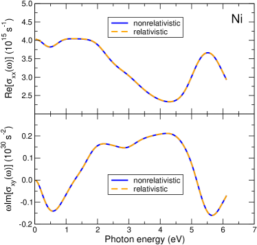
Figure 1: (Color online) Calculated optical conductivity spectra ${\rm Re}[\sigma_{xx}(\omega)]$ (top panel) and $\omega{\rm Im}[\sigma_{xy}(\omega)]$ (bottom panel) of fcc Ni, using the relativistic and nonrelativistic current density formulations. The blue lines are calculated considering the momentum operator in nonrelativistic approximation ($\bm{p}=-i\hbar\bm{\nabla}$). The orange dotted-dashed lines are the calculations performed using Eq. (14) as momentum operator.

In Fig. 1 we show the comparison between the interband-only optical conductivity elements, ${\rm Re}[\sigma_{xx}(\omega)]$ and $\omega{\rm Im}[\sigma_{xy}(\omega)]$, computed with the nonrelativistic momentum operator as well as with including the relativistic corrections to the momentum operator. The calculations are performed with a broadening $\hbar/\tau=0.03$ Ry. As it is apparent from the plot the contribution due to the relativistic terms does not lead to an appreciable change in the conductivity spectra. The influence of the additional light-spin interaction terms on the MOKE spectra is shown in Fig. 2. As expected from the results shown in Fig. 1, the comparison in Fig. 2 shows that, also for the Kerr spectra, the contribution from the relativistic correction terms is very small.

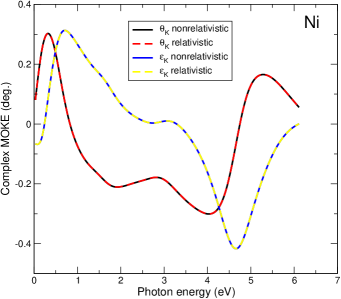
Figure 2: (Color online) Calculated magneto-optical Kerr rotation and Kerr ellipticity of Ni. The black and blue lines are, respectively, the Kerr rotation $\theta_{\rm K}$ and ellipticity $\varepsilon_{\rm K}$ calculated without taking into account the additional relativistic terms of the momentum operator. The red and yellow dashed lines are the Kerr rotation and ellipticity, respectively, calculated retaining the relativistic terms of the momentum operator.

To quantify the influence of the relativistic terms on the conductivity tensor we show in Fig. 3 (top panel) the difference between the off-diagonal components of the conductivity tensor calculated with and without the relativistic terms in the momentum operator. This difference is of the order of $10^{-4}$ ($\times 10^{15}$ s^-1) for both the real and imaginary part. Note that the difference curves in Fig. 3 are very smooth and do not show any jitter. The reason for its absence is the high numerical accuracy in the calculation of $\sigma_{xy}(\omega)$ which is still appreciably higher (better than $10^{-7}$) (for details of the numerical implementation, see Oppeneer et al. (1992a)). Hence, there is no doubt that we can adequately capture the influence of the relativistic corrections terms. In Fig. 3 (bottom panel) we plot the absolute values of the differences in $\sigma_{xy}$ normalized to the nonrelativistic off-diagonal conductivity, i.e., $|\Delta\sigma_{xy}|/|\sigma_{xy,\rm{nr}}|$, and the same for the complex Kerr angle, i.e., $|\Delta\Phi_{\rm K}|/|\Phi_{\rm K,nr}|=$ $(\Delta\theta_{\rm K}^{2}+\Delta\varepsilon_{\rm K}^{2})^{1/2}/(\theta_{\rm K,nr}^{2}+\varepsilon_{\rm K,nr}^{2})^{1/2}$. For both quantities the normalized differences are of the order of 0.1%. Thus, we can conclude that the relativistic spin-photon terms do contribute to the magneto-optical signal of Ni, but that this contribution is rather small. The spin-photon induced change in the MOKE signal would consequently be present during the pump pulse, where it would be interpreted as as magnetization change of the order of 0.1%.

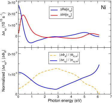
Figure 3: (Color online) Top panel: differences between the off-diagonal conductivity $\sigma_{xy}(\omega)$ components computed with the relativistic and the nonrelativistic current operators. Bottom panel: calculated absolute value of the difference in $\sigma_{xy}$ ($\Phi_{\rm K}$) normalized to the quantities $|\sigma_{xy,{\rm nr}}|$ ($|\Phi_{\rm K,nr}|$) computed with the nonrelativistic momentum operator.

IV Discussion and Conclusions

Previous estimations of the influence of the relativistic spin-photon interaction have been made by Vonesch and Bigot Vonesch and Bigot (2012), who considered optical transitions on a hydrogen atom within the framework of an extended Pauli Hamiltonian. Calculating the matrix elements of the spin-photon terms in their Hamiltonian, they found that these were of the order of $1\times 10^{-6}$ (whereas the nonrelativistic term $\bm{p}\cdot\bm{A}$ was of order 1). The largest contribution in their treatment originated from the cross term $\bm{A}_{L}\cdot\bm{A}_{\rm ext}$ of the vector potential of the laser radiation and an external magnetic field, which, as mentioned before, does not arise in our treatment. Vonesch and Bigot estimated a change in the normalized Kerr rotation of $0.5\times 10^{-3}$. Thus, even with the additional term this estimated change in the Kerr rotation is in overall accord with ours for metallic Ni.

Nonetheless, in spite of the nonzero influence, our ab initio calculations do not evidence that relativistic light-induced spin-flip transitions could provide a notable demagnetization channel. They would appear as a small demagnetization effect during the pump pulse which is in experiments typically about 70 fs wide. However, during and immediately after the pump pulse there will also be the influence of “bleaching”, that is, the reduction in the optical excitation channels caused by the presence of pump-laser excited electrons Koopmans et al. (2000); Guidoni et al. (2002). The influence of such nonequilibrium electron populations on the MOKE spectra of Ni have been evaluated previously Oppeneer and Liebsch (2004), yet without the here-investigated relativistic spin-photon effects, and were found to be significant. We can thus conclude that the nonequilibrium populations have a larger effect on the apparent MOKE signal than the relativistic spin-photon interaction.

The demagnetization of Ni after an intensive laser pulse has recently been computed by Krieger et al. Krieger et al. (2014), who employed the time-dependent DFT formalism. Assuming extremely intense electromagnetic fields with a laser intensity of $10^{14}-10^{15}$ W/m² they computed an appreciably larger demagnetization (of $\sim 50$ %) than we do, which they attribute to dominance of nonlinear effects. Conversely, in the current investigation we are in the moderate fluency regime, with typical laser intensities of $\simeq 10^{11}$ W/m², where the linear interaction Hamiltonian Eq. (11) should be sufficient and there is only a small number of electrons present in the excited state; for this regime our results should be valid.

Summarizing, we performed the Foldy-Wouthuysen transformation on the Dirac-Kohn-Sham equation in the presence of the exchange magnetic field as it is required for the relativistic density functional theory in the framework of the local spin density approximation. We obtained a Hamiltonian where several terms are consistent with results derived previously in Ref. Crépieux and Bruno (2001). We further showed that the spin-polarized term in the current density operator is irrelevant for the calculation of the conductivity spectra. We discussed the modification caused by the relativistic spin-photon terms to the linear-response theory for the conductivity, and showed that an identical linear-response expression can be obtained for the nonrelativistic, semirelativistic and fully relativistic interaction Hamiltonians. We then calculated the influence of the relativistic correction terms to the magneto-optical Kerr spectra of nickel. In the moderate fluency regime, where the linear-response theory is expected to be valid we find that relativistic spin-photon interactions can give a small modification ($\leq 0.1$ %) of the off-diagonal optical conductivity and of the MOKE signal. Thus, our calculations confirm that relativistic spin-photon interactions do exist, as originally proposed in Ref. Bigot et al., 2009, but we do not find that these could provide a notable channel of laser-induced magnetization loss.

Appendix A The Pauli Hamiltonian

In the presence of an external electromagnetic field (characterized by the vector potential $\bm{A}(\bm{r},t)$), the fully relativistic Dirac Hamiltonian (first without exchange field) has the form

$$H=c\bm{\alpha}\cdot\left(\bm{p}-e\bm{A}\right)+\left(\bm{\beta}-\mathbb{1}\right)mc^{2}+V.$$ (19)

In the nonrelativistic limit (which is obtained by performing the FW transformation), it exactly gives the Pauli Hamiltonian

$$H_{\rm P}=\frac{\left(\bm{p}-e\bm{A}\right)^{2}}{2m}+V-\frac{e\hbar}{2m}\bm{\sigma}\cdot\bm{B},$$ (20)

where the external magnetic field is given by $\bm{B}=\bm{\nabla}\times\bm{A}$. If we choose for simplicity a gauge such that

$$\bm{A}=\frac{\bm{B}\times\bm{r}}{2},$$

which fulfills the Coulomb gauge ($\bm{\nabla}\cdot\bm{A}=0$) for the uniform magnetic field. Then, with this Pauli Hamiltonian one can show how the different magnetic contributions arise. Namely, the Pauli Hamiltonian can be rewritten as

$$H_{\rm P}=\left(\frac{p^{2}}{2m}+V\right)-\mu_{B}\,\bm{B}\cdot\left(\bm{L}+g\bm{S}\right)+\frac{e^{2}}{8m}\left(\bm{B}\times\bm{r}\right)^{2},$$ (21)

with $g$ the Landé g-factor, which is 2 for spin degrees of freedom. The first term obviously is the unperturbed Hamiltonian, the dominant perturbation is the paramagnetic contribution and the last term is the diamagnetic contribution Blundell (2001). Note that the external magnetic field couples to both the spin and orbital angular momentum operators, as it should be.

For magnetic materials the Pauli exclusion principle gives in addition rise to magnetic exchange. To include magnetic exchange (which dominates over the dipole-dipole interaction) the DKS Hamiltonian has to be written as Eschrig (1996)

$$H=c\,\bm{\alpha}\cdot\left(\bm{p}-e\bm{A}\right)+\left({\bm{\beta}}-\mathbb{1}\right)mc^{2}+V+\mu_{B}{\bm{\beta}}\,\bm{\Sigma}\cdot\bm{B}^{\rm xc},$$ (22)

where the exchange field $\bm{B}^{\rm xc}$ has to be separated from the external magnetic vector potential as it would otherwise couple to the orbital degrees of freedom. The FW transformation of this Hamiltonian leads to the Hamiltonian given in Eq. (9).

Appendix B Derivation of the optical conductivity

Introducing the electromagnetic field $\bm{A}(\bm{r},t)$ produced by the intensive laser pulse the first-order interaction Hamiltonian could be written in terms of the momentum operator [Eq. (14)] of the unperturbed Hamiltonian,

$$H_{I}=-\frac{e}{m}\bm{\Pi}\cdot\bm{A}.$$ (23)

This form of the interaction enters in the nonrelativistic, semirelativistic and fully relativistic cases. Here we consider the semirelativistic case corresponding to the extended Pauli Hamiltonian. We also note that, using a proper gauge, $\bm{A}=\frac{\bm{B}\times\bm{r}}{2}$, the above mentioned Hamiltonian can be rewritten as first-order interaction Hamiltonian in $\bm{E}(\bm{r},t)$. Using the gauge, it is obvious that $\bm{r}\cdot\bm{A}=0$, which gives

$$\frac{d}{dt}(\bm{r}\cdot\bm{A}) = 0\Rightarrow\dot{\bm{r}}\cdot\bm{A}=\bm{r}\cdot\bm{E}$$ (24)

$$\Rightarrow\frac{e}{m}\bm{\Pi}\cdot\bm{A}=e\bm{r}\cdot\bm{E}.$$

Therefore, the first-order interaction Hamiltonian can equally well be written in the form:

$$H_{I}=-e\sum_{i}\bm{r}_{i}\cdot\bm{E}\equiv Be^{-i\omega^{+}t},$$ (25)

where $\bm{r}_{i}$ are the positions of the electrons and $\omega^{+}\equiv\omega+i/\tau$. In linear-response theory the total average, induced current $\bm{J}=\bm{j}V$, with $V$ the volume of the system, is computed from (see, e.g. Callaway (1974)):

$$J(t)=\textrm{Tr}(\rho_{0}J)+\frac{1}{i\hbar}\int_{-\infty}^{t}\!dt^{\prime}\big{\langle}\left[J(t),H_{I}(t^{\prime})\right]\big{\rangle}_{0},$$ (26)

where $\langle...\rangle_{0}$ means that the average has to be computed with the equilibrium density matrix $\rho_{0}$. The first term refers to the equilibrium current density, which is usually taken to be zero in linear-response theory. Note however the difference to the derivation given in Refs. Callaway (1974); Landau and Lifshitz (1981), where this is not done and a second-order interaction term $\bm{A}^{2}$ is introduced in the Hamiltonian Landau and Lifshitz (1981). This term is rewritten in Refs. Callaway (1974); Landau and Lifshitz (1981) and leads to the Drude response (first term in (28) below). Such term should however not be included in a linear-response treatment, and it is actually not needed, as our derivation shows. Our formalism is valid in nonrelativistic, semirelativistic and fully relativistic case. We introduce the linear interaction Hamiltonian according to (25) in the second term of Eq. (26) and calculate the integral. Partial integration of this second term leads to:

$$J_{\alpha}(t) = \frac{1}{i\hbar}\big{\langle}\left[J_{\alpha}(t),B(t)\right]\big{\rangle}_{0}\frac{e^{-i\omega^{+}t}}{-i\omega^{+}}$$ (27)

$$- \frac{1}{i\hbar}\int_{-\infty}^{t}dt^{\prime}\big{\langle}[J_{\alpha}(t),\dot{B}(t^{\prime})]\big{\rangle}_{0}\frac{e^{-i\omega^{+}t^{\prime}}}{-i\omega^{+}},$$

where $\dot{B}$ is the derivative of $B$, which is related to the current, $\dot{B}(t)=-e\sum_{i}\dot{\bm{r}_{i}}(t)\cdot\bm{E}=-\bm{J}(t)\cdot\bm{E}$. Using Eq. (25) we calculate the commutators and it is evident that the integral leads to the current-current correlation in the average current,

$$\!\!\!\!\!\!\!\!\!J_{\alpha}(t) = \frac{iNe^{2}}{m\omega^{+}}E_{\alpha}(t)e^{-i\omega^{+}t}$$ (28)

$$- \frac{1}{i\hbar}\int_{-\infty}^{t}\!\!\!dt^{\prime}\big{\langle}\left[J_{\alpha}(t),J_{\beta}(t^{\prime})\right]\big{\rangle}_{0}\frac{E_{\beta}(t^{\prime})e^{-i\omega^{+}t^{\prime}}}{i\omega^{+}}.$$

The conductivity response to the electromagnetic field is given as

$$j_{\alpha}(t)=\int_{-\infty}^{t}\!dt^{\prime}\sigma_{\alpha\beta}(t-t^{\prime})E_{\beta}(t^{\prime}).$$ (29)

Now, comparing both equations we obtain the linear-response expression for the conductivity. Computed in Fourier space, the conductivity in terms of (noninteracting) single-particle states is then (see Ref. Oppeneer (2001) for details)

$$\sigma_{\alpha\beta}(\omega) = \frac{ie^{2}N\delta_{\alpha\beta}}{Vm\omega^{+}}$$ (30)

$$+ \frac{i}{V\hbar\omega^{+}}\sum_{nn^{\prime}}\frac{f(\epsilon_{n})-f(\epsilon_{n^{\prime}})}{{\omega^{+}-\omega_{n^{\prime}n}}}j^{\alpha}_{nn^{\prime}}j^{\beta}_{n^{\prime}n},$$

where $j_{nn^{\prime}}$ are the matrix elements of the current density operator for the single-particle states $n$ and $n^{\prime}$, $f(\epsilon_{n})$ is the Fermi-Dirac distribution function of the $n$-th state having energy $\epsilon_{n}$ and $\hbar\omega_{n^{\prime}n}=\epsilon_{n^{\prime}}-\epsilon_{n}$. This linear-response expression is exact for the non-relativistic, semirelativistic and fully relativistic cases. In the semirelativistic limit, the two terms in Eq. (30) can be approximately joined together, which yields

$$\sigma_{\alpha\beta}(\omega)\approx-\frac{i}{\hbar V}\sum_{nn^{\prime}}\frac{f(\epsilon_{n})-f(\epsilon_{n^{\prime}})}{\omega_{nn^{\prime}}}\frac{j^{\alpha}_{n^{\prime}n}j^{\beta}_{nn^{\prime}}}{\omega-\omega_{nn^{\prime}}+{i}/{\tau}},$$ (31)

where the $\approx$ sign relates to the intraband term i.e., $n=n^{\prime}$) for which the approximation $\bm{\Pi}_{\rm P}\approx\bm{p}$ has been made.

Appendix C Derivation of the spin-polarized current

The current density operator in semirelativistic form was previously shown Nowakowski (1999); Huszár (1967) to contain a term $\bm{j}_{sp}=-\frac{ie}{2m}(\overleftarrow{\bm{p}}\times\bm{\sigma}+\bm{\sigma}\times{\bm{p}})$. This term also appears in our treatment. When we apply the FW transformation to the DKS Hamiltonian in Eq. (2), we find a term $\frac{i}{2m}\bm{\sigma}\cdot(\bm{p}\times\bm{p})$, in the Hamiltonian. This term is taken to be zero for obvious reasons. However, it is this term that leads to the spin-polarized current density $\bm{j}_{sp}$.

Defining the charge density as $\rho=e\delta\left(\bm{r}-\hat{\bm{r}}\right)$ and using the Heisenberg equation of motion for the above-given Hamiltonian term,

$$\frac{d\rho}{dt} = \frac{1}{i\hbar}\left[e\delta\left(\bm{r}-\hat{\bm{r}}\right),\frac{i}{2m}\bm{\sigma}\cdot(\bm{p}\times\bm{p})\right]$$ (32)

$$= \frac{e}{2m\hbar}\bm{\sigma}\cdot\left\{\left[\delta\left(\bm{r}-\hat{\bm{r}}\right),\bm{p}\right]\times\bm{p}+\bm{p}\times\left[\delta\left(\bm{r}-\hat{\bm{r}}\right),\bm{p}\right]\right\}$$

$$= \bm{\nabla}\cdot\frac{ie}{2m}\left\{\bm{\bm{\sigma}}\times\bm{p}+\overleftarrow{\bm{p}}\times\bm{\bm{\sigma}}\right\}$$

$$= -\bm{\nabla}\cdot\bm{j}_{sp}.$$

In this derivation, we make use of the fact that, the commutator in the position basis, $\left[\delta\left(\bm{r}-\hat{\bm{r}}\right),\bm{p}\right]=i\hbar|\bm{r}\rangle\bm{\nabla}_{\bm{r}}\langle\bm{r}|$. Using the continuity equation we extract the spin-polarized current density operator as ${\bm{j}}_{sp}=-\frac{ie}{2m}\{\bm{\sigma}\times\bm{p}+\overleftarrow{\bm{p}}\times{\bm{\sigma}}\}$. The matrix elements are given by:

$$\!\!\langle\Psi_{n}|\bm{j}_{sp}|\Psi_{m}\rangle = -\frac{e\hbar}{2m}\int_{V}\!\!d\bm{r}\left\{\Psi_{n}^{*}\bm{\sigma}\times\bm{\nabla}\Psi_{m}\!-\!\Psi_{m}\bm{\nabla}\Psi_{n}^{*}\times\bm{\sigma}\right\}$$ (33)

$$= \frac{e\hbar}{2m}\int_{V}\!\!d\bm{r}\bm{\nabla}\times\left[\Psi_{n}^{*}\bm{\sigma}\Psi_{m}\right].$$

References

- Beaurepaire et al. (1996) E. Beaurepaire, J.-C. Merle, A. Daunois, and J.-Y. Bigot, Phys. Rev. Lett. 76, 4250 (1996).
- Hohlfeld et al. (1997) J. Hohlfeld, E. Matthias, R. Knorren, and K. H. Bennemann, Phys. Rev. Lett. 78, 4861 (1997).
- Scholl et al. (1997) A. Scholl, L. Baumgarten, R. Jacquemin, and W. Eberhardt, Phys. Rev. Lett. 79, 5146 (1997).
- Regensburger et al. (2000) H. Regensburger, R. Vollmer, and J. Kirschner, Phys. Rev. B 61, 14716 (2000).
- Kampfrath et al. (2002) T. Kampfrath, R. G. Ulbrich, F. Leuenberger, M. Münzenberg, B. Sass, and W. Felsch, Phys. Rev. B 65, 104429 (2002).
- van Kampen et al. (2005) M. van Kampen, J. T. Kohlhepp, W. J. M. de Jonge, B. Koopmans, and R. Coehoorn, J. Phys.: Condens. Matter 17, 6823 (2005).
- Cheskis et al. (2005) D. Cheskis, A. Porat, L. Szapiro, O. Potashnik, and S. Bar-Ad, Phys. Rev. B 72, 014437 (2005).
- Carley et al. (2012) R. Carley, K. Döbrich, B. Frietsch, C. Gahl, M. Teichmann, O. Schwarzkopf, P. Wernet, and M. Weinelt, Phys. Rev. Lett. 109, 0574012 (2012).
- Boeglin et al. (2010) C. Boeglin, E. Beaurepaire, V. Halté, V. López-Flores, C. Stamm, N. Pontius, H. A. Dürr, and J.-Y. Bigot, Nature 465, 458 (2010).
- Radu et al. (2011) I. Radu, K. Vahaplar, C. Stamm, T. Kachel, N. Pontius, H. A. Duerr, T. A. Ostler, J. Barker, R. F. L. Evans, R. W. Chantrell, A. Tsukamoto, A. Itoh, A. Kirilyuk, Th. Rasing, and A. V. Kimel, Nature 472, 205 (2011).
- Mathias et al. (2012) S. Mathias, C. La-O-Vorakiat, P. Grychtol, P. Granitzka, E. Turgut, J. M. Shaw, R. Adam, H. T. Nembach, M. E. Siemens, S. Eich, C. M. Schneider, T. J. Silva, M. Aeschlimann, M. M. Murnane, and H. C. Kapteyn, Proc. Natl. Acad. Scie. USA 109, 4792 (2012).
- Rudolf et al. (2012) D. Rudolf, C. La-O-Vorakiat, M. Battiato, R. Adam, J. M. Shaw, E. Turgut, P. Maldonado, S. Mathias, P. Grychtol, H. T. Nembach, T. J. Silva, M. Aeschlimann, H. C. Kapteyn, M. M. Murnane, C. M. Schneider, and P. M. Oppeneer, Nature Commun. 3, 1037 (2012).
- Eschenlohr et al. (2013) A. Eschenlohr, M. Battiato, P. Maldonado, N. Pontius, T. Kachel, K. Holldack, R. Mitzner, A. Föhlisch, P. M. Oppeneer, and C. Stamm, Nature Mater. 12, 332 (2013).
- Bergeard et al. (2014) N. Bergeard, V. López-Flores, V. Halté, M. Hehn, C. Stamm, N. Pontius, E. Beaurepaire, and C. Boeglin, Nature Commun. 5, 3466 (2014).
- Bovensiepen (2009) U. Bovensiepen, Nat. Phys. 5, 461 (2009).
- Kirilyuk et al. (2010) A. Kirilyuk, A. V. Kimel, and Th. Rasing, Rev. Mod. Phys. 82, 2731 (2010).
- Carva et al. (2011a) K. Carva, M. Battiato, and P. M. Oppeneer, Nature Phys. 7, 665 (2011a).
- Zhang and Hübner (2000) G. P. Zhang and W. Hübner, Phys. Rev. Lett. 85, 3025 (2000).
- Carpene et al. (2008) E. Carpene, E. Mancini, C. Dallera, M. Brenna, E. Puppin, and S. De Silvestri, Phys. Rev. B 78 (2008).
- Koopmans et al. (2010) B. Koopmans, G. Malinowski, F. Dalla Longa, D. Steiauf, M. Faehnle, T. Roth, M. Cinchetti, and M. Aeschlimann, Nature Mater. 9, 259 (2010).
- Krauss et al. (2009) M. Krauss, T. Roth, S. Alebrand, D. Steil, M. Cinchetti, M. Aeschlimann, and H. C. Schneider, Phys. Rev. B 80, 180407(R) (2009).
- Battiato et al. (2010) M. Battiato, K. Carva, and P. M. Oppeneer, Phys. Rev. Lett. 105, 027203 (2010).
- Battiato et al. (2012) M. Battiato, K. Carva, and P. M. Oppeneer, Phys. Rev. B 86, 024404 (2012).
- Zhang et al. (2009) G. P. Zhang, W. Hübner, G. Lefkidis, Y. Bai, and T. F. George, Nature Phys. 5, 499 (2009).
- Bigot et al. (2009) J.-Y. Bigot, M. Vomir, and E. Beaurepaire, Nature Phys. 5, 515 (2009).
- Atxitia et al. (2010) U. Atxitia, O. Chubykalo-Fesenko, J. Walowski, A. Mann, and M. Münzenberg, Phys. Rev. B 81, 174401 (2010).
- Ostler et al. (2012) T. A. Ostler, J. Barker, R. F. L. Evans, R. W. Chantrell, U. Atxitia, O. Chubykalo-Fesenko, S. El Moussaoui, L. Le Guyader, E. Mengotti, L. J. Heyderman, F. Nolting, A. Tsukamoto, A. Itoh, D. Afanasiev, B. A. Ivanov, A. M. Kalashnikova, K. Vahaplar, J. Mentink, A. Kirilyuk, Th. Rasing, and A. V. Kimel, Nature Commun. 3, 666 (2012).
- Wienholdt et al. (2013) S. Wienholdt, D. Hinzke, K. Carva, P. M. Oppeneer, and U. Nowak, Phys. Rev. B 88, 020406 (2013).
- Bar’yakhtar et al. (2013) V. G. Bar’yakhtar, V. I. Butrim, and B. A. Ivanov, JETP Lett. 98, 289 (2013).
- Carva et al. (2011b) K. Carva, M. Battiato, and P. M. Oppeneer, Phys. Rev. Lett. 107, 207201 (2011b).
- Essert and Schneider (2011) S. Essert and H. C. Schneider, Phys. Rev. B 84, 224405 (2011).
- Carva et al. (2013) K. Carva, M. Battiato, D. Legut, and P. M. Oppeneer, Phys. Rev. B 87, 184425 (2013).
- Illg et al. (2013) C. Illg, M. Haag, and M. Fähnle, Phys. Rev. B 88, 214404 (2013).
- Schellekens and Koopmans (2013) A. J. Schellekens and B. Koopmans, Phys. Rev. Lett. 110, 217204 (2013).
- Mueller et al. (2013) B. Y. Mueller, A. Baral, S. Vollmar, M. Cinchetti, M. Aeschlimann, H. C. Schneider, and B. Rethfeld, Phys. Rev. Lett. 111, 167204 (2013).
- Haag et al. (2014) M. Haag, C. Illg, and M. Fähnle, Phys. Rev. B 90, 014417 (2014).
- Dixit et al. (2013) A. Dixit, Y. Hinschberger, J. Zamanian, G. Manfredi, and P.-A. Hervieux, Phys. Rev. A 88, 032117 (2013).
- Hinschberger and Hervieux (2013) Y. Hinschberger and P.-A. Hervieux, Phys. Rev. B 88, 134413 (2013).
- Vonesch and Bigot (2012) H. Vonesch and J.-Y. Bigot, Phys. Rev. B 85, 180407 (2012).
- MacDonald and Vosko (1979) A. H. MacDonald and S. H. Vosko, J. Phys. C: Solid State Phys. 12, 2977 (1979).
- Eschrig and Servedio (1999) H. Eschrig and V. D. P. Servedio, J. Comput. Chem. 20, 23 (1999).
- Greiner (2000) W. Greiner, Relativistic quantum mechanics. Wave equations (Springer, Berlin, 2000).
- Kraft et al. (1995) T. Kraft, P. M. Oppeneer, V. N. Antonov, and H. Eschrig, Phys. Rev. B 52, 3561 (1995).
- Foldy and Wouthuysen (1950) L. L. Foldy and S. A. Wouthuysen, Phys. Rev. 78, 29 (1950).
- Crépieux and Bruno (2001) A. Crépieux and P. Bruno, Phys. Rev. B 64, 094434 (2001).
- Oppeneer (2001) P. M. Oppeneer, in Handbook of Magnetic Materials, Vol. 13, edited by K. H. J. Buschow (Elsevier, Amsterdam, 2001) pp. 229 – 422.
- Landau and Lifshitz (1981) L. D. Landau and L. M. Lifshitz, Quantum Mechanics: Non-Relativistic Theory, 3rd ed., Vol. 3 (Butterworth-Heinemann, Oxford, 1981).
- Nowakowski (1999) M. Nowakowski, Am. J. Phys. 67, 916 (1999).
- Huszár (1967) M. Huszár, Acta Phys. Acad. Scien. Hungaricae 23, 225 (1967).
- Ullrich (2011) C. A. Ullrich, Time-dependent density-functional theory: Concepts and applications (Oxford University Press, Oxford, 2011).
- Marques et al. (2012) M. A. Marques, N. T. Maitra, F. M. Nogueira, E. K. U. Gross, and A. Rubio, eds., Fundamentals of Time-Dependent Density Functional Theory, Lecture Notes in Physics, Vol. 837 (Springer, Heidelberg, 2012).
- Koopmans et al. (2000) B. Koopmans, M. van Kampen, J. T. Kohlhepp, and W. J. M. de Jonge, Phys. Rev. Lett. 85, 844 (2000).
- Oppeneer et al. (1992a) P. M. Oppeneer, T. Maurer, J. Sticht, and J. Kübler, Phys. Rev. B 45, 10924 (1992a).
- Argyres (1955) P. N. Argyres, Phys. Rev. 97, 334 (1955).
- Oppeneer et al. (1992b) P. M. Oppeneer, J. Sticht, T. Maurer, and J. Kübler, Z. Physik B 88, 309 (1992b).
- Williams et al. (1979) A. R. Williams, J. Kübler, and C. D. Gelatt, Phys. Rev. B 19, 6094 (1979).
- Guidoni et al. (2002) L. Guidoni, E. Beaurepaire, and J.-Y. Bigot, Phys. Rev. Lett. 89 (2002).
- Oppeneer and Liebsch (2004) P. M. Oppeneer and A. Liebsch, J. Phys.: Condens. Matter 16, 5519 (2004).
- Krieger et al. (2014) K. Krieger, J. K. Dewhurst, P. Elliott, S. Sharma, and E. K. U. Gross, cond-mat arXiv:1406.6607v1 (2014).
- Blundell (2001) S. Blundell, Magnetism in Condensed Matter (Oxford University Press, Oxford, 2001).
- Eschrig (1996) H. Eschrig, The Fundamentals of Density Functional Theory (Teubner Verlag, Leipzig, 1996).
- Callaway (1974) J. Callaway, Quantum Theory of the Solid State, 2nd ed. (Academic Press, San Diego, 1974) pp. 465 – 572.