On Temporal Graph Exploration

Abstract

A temporal graph is a graph in which the edge set can change from one time step to the next. The temporal graph exploration problem TEXP is the problem of computing a foremost exploration schedule for a temporal graph, i.e., a temporal walk that starts at a given start node, visits all nodes of the graph, and has the smallest arrival time. In the first part of the paper, we consider only undirected temporal graphs that are connected at each time step. For such temporal graphs with $n$ nodes, we show that it is $\mathbf{NP}$-hard to approximate TEXP with ratio $O(n^{1-\varepsilon})$ for every $\varepsilon>0$. We also provide an explicit construction of temporal graphs that require $\Theta(n^{2})$ time steps to be explored.

In the second part of the paper, we still consider temporal graphs that are connected in each time step, but we assume that the underlying graph (i.e. the graph that contains all edges that are present in the temporal graph in at least one time step) belongs to a specific class of graphs. Among other results, we show that temporal graphs can be explored in $O(n^{1.5}k^{1.5}\log n)$ time steps if the underlying graph has treewidth $k$, in $O(n^{1.8}\log n)$ time steps if the underlying graph is planar, and in $O(n\log^{3}n)$ time steps if the underlying graph is a $2\times n$ grid.

In the third part of the paper, we consider settings where the graphs in future time steps are not known and the exploration schedule is constructed online. We replace the connectedness assumption by a weaker assumption and show that $m$-edge temporal graphs with regularly present edges and with probabilistically present edges can be explored online in $O(m)$ time steps and $O(m\log n)$ time steps with high probability, respectively. We finally show that the latter result can be used to obtain a distributed algorithm for the gossiping problem in random temporal graphs.

Keywords: non-approximability, planar graphs, bounded treewidth, regularly present edges, random edges, distributed algorithm, gossiping problem

ACM classification: C.2.4; F.2.2; G.2.2

1 Introduction

Many networks are not static and change over time. For example, connections in a transport network may only operate at certain times. Connections in social networks are created and removed over time. Links in wired or wireless networks may change dynamically. Dynamic networks have been studied in the context of faulty networks, scheduled networks, time-varying networks, distributed algorithms, etc. For an overview, we refer to [9], [30], [32], and [35]. We consider a model of time-varying networks called temporal graphs. A temporal graph $\mathcal{G}$ is given by a sequence of undirected graphs $G_{0}=(V,E_{0})$, $G_{1}=(V,E_{1})$, $G_{2}=(V,E_{2})$, …, $G_{L}=(V,E_{L})$ that all share the same vertex set $V$, but whose edge sets may differ. The number $L$ is called the lifetime of $\mathcal{G}$. In Sections 3 and 4, we assume that the whole temporal graph is presented to the algorithm.

In temporal graphs, the natural notion of moving through the graph using at most one edge in each time step leads to the concept of temporal paths. Standard algorithms for well known path-related problems such as connected components, diameter, reachability, shortest paths, graph exploration, etc. cannot be used directly in temporal graphs, as temporal paths behave quite differently from paths in static graphs. For instance, Berman [4] observed that the vertex version of Menger’s theorem does not hold for temporal graphs. Moreover, algorithms for path problems in static graphs usually have a natural objective to optimize (the length of the path or tour), whereas temporal graphs allow us to consider different possible objectives. For example, Bui-Xuan, Ferreira, and Jarry [8] search for a shortest, a foremost, or a fastest $s$-$t$-path, i.e., a temporal path from $s$ to $t$ with a minimal number of edges, earliest arrival time, or a shortest duration, respectively.

We consider the temporal graph exploration problem, introduced by Michail and Spirakis [33] and denoted TEXP, whose goal is to compute an exploration schedule (or temporal walk) with the earliest arrival time such that an agent can visit all vertices in $V$. The agent is initially located at a start node $s\in V$. In time step $i$ ($i\geq 0$) the agent can either remain at its current node or move to an adjacent node via an edge that is present in $E_{i}$. Unless we consider an online variant of TEXP we always assume that we know the graphs of all time steps in advance.

We remark that static undirected graphs can easily be explored in less than $2|V|$ steps using depth-first search, while there are static directed graphs for which exploration requires $\Theta(|V|^{2})$ steps.

Some work on dynamic networks considers temporal graphs whose edges appear with some kind of periodicity [10, 29] or graphs whose edges appear or fail with a certain probability [1, 24, 26]. Except in Sections 5-7 we do not assume that edges appear with some periodicity or certain probabilistic properties. Instead, unless stated otherwise, we only assume that the given temporal graph is always connected, meaning that each of the graphs $G_{i}$ for $0\leq i\leq L$ is a connected graph in the standard sense. Michail and Spirakis [33] observe that without such an assumption, it is even $\mathbf{NP}$-complete to decide if the graph can be explored at all. They also show that, under this connectedness assumption, every temporal graph with $n$ vertices can be explored with an arrival time of at most $n^{2}$. We focus on the case where an exploration schedule always exists and assume throughout this paper that the lifetime of the given temporal graph is at least $|V|^{2}$.

A $\rho$-approximation algorithm for TEXP is an algorithm that runs in polynomial time and outputs an exploration schedule whose arrival time is at most $\rho$ times the arrival time of the optimal exploration schedule. Michail and Spirakis also prove that there is no $(2-\varepsilon)$-approximation for TEXP for any $\varepsilon>0$ unless $\mathbf{P}$ = $\mathbf{NP}$. They define the dynamic diameter of a temporal graph to be the minimum integer $d$ such that for every time $i$ and every vertex $v$, every other vertex $w$ can be reached in $d$ time steps on a temporal walk that starts at $v$ at time $i$. They provide a $d$-approximation algorithm for TEXP, where $d$ is the dynamic diameter of the temporal graph. We note that $d$ can be as large as $n-1$, and hence the approximation ratio of their algorithm in terms of $n$ is only $n-1$. Thus, there is a significant gap between the lower bound of $2-\varepsilon$ and the upper bound of $n-1$ on the best possible approximation ratio, which we address in this paper.

Our contributions

We close the gap between the upper and lower bound on the approximation ratio of TEXP by proving that it is $\mathbf{NP}$-hard to approximate TEXP with ratio $O(n^{1-\varepsilon})$ for every $\varepsilon>0$. Furthermore, we provide an explicit construction of temporal graphs that require $\Theta(n^{2})$ time steps to be explored. We also prove that the problem is $\mathbf{NP}$-hard to approximate with ratio $O(\Delta^{1-\varepsilon})$ for every $\varepsilon>0$ if the underlying graph (i.e., the graph that contains all edges that are present in the temporal graph in at least one time step) has degree $\Delta=\Omega(n^{\delta})$ for any constant $\delta>0$.

We then consider TEXP under the assumption that the underlying graph belongs to a specific class of graphs. We present an exploration method for temporal graphs whose underlying graphs can be split into “small” components using “small” separators. This allows us to show that temporal graphs can be explored in $O(n^{1.5}k^{1.5}\log n)$ time steps if the underlying graph has treewidth $k$ and in $O(n^{1.8}\log n)$ time steps if the underlying graph is planar. Furthermore, we show that temporal graphs can be explored in $O(n\log^{3}n)$ time steps if the underlying graph is a $2\times n$ grid and in $O(n)$ time steps if the underlying graph is a cycle or a cycle with a chord. Several of these results use a technique by which we specify an exploration schedule for multiple agents and then apply a general reduction from the multi-agent case to the single-agent case. We also show that temporal graphs exist where the underlying graph is a bounded-degree planar graph and each $G_{i}$ is a path such that the optimal arrival time of the exploration walk is $\Omega(n\log n)$.

After this, we consider a setting where the edges of the underlying graph are present with a certain regularity or with a certain probability, and the algorithm does not have full knowledge of the edges that are present in each future time step. Thus, the exploration schedule needs to be determined online. We show that it is possible to determine an exploration schedule online that explores $m$-edge temporal graphs with an arrival time of $O(m)$ for regularly present edges or $O(m\log n)$ for probabilistically present edges (the latter holds with high probability).

As an application of our graph-exploration algorithm on random temporal graphs, we present a distributed algorithm for the so-called gossiping problem [5, 11, 21]. In the gossiping problem, every vertex of a graph has to communicate a private value to all the other vertices. Thus, $\Omega(n)$ messages between neighbors are required even if a connected $n$-vertex graph is given that does not change over time. Ignoring special cases of negligible probability, we show that, after some initialization using $O(m\log^{2}n)$ messages, we can solve instances of the gossiping problem with $O(m\log n)$ messages per instance on an $n$-vertex $m$-edge graph $G$ that is “connected” (in a certain sense). If $G$ is sparse (i.e., $m=O(n)$), we thus need only a factor of $O(\log n)$ more messages than the lower bound of $\Omega(n)$ to solve an instance of the problem.

The remainder of the paper is structured as follows. Related work is discussed in Section 1.1. In Section 2, we give some definitions and preliminary results. Section 3 presents our inapproximability results for general temporal graphs and for temporal graphs whose underlying graph has maximum degree $\Delta$. The results for temporal graphs with restricted underlying graphs are given in Section 4. Temporal graphs with regularly present edges and probabilistically present edges are considered in Sections 5 and 6, respectively. The distributed algorithm for the gossiping problem is given in Section 7. Section 8 concludes the paper.

1.1 Related work

The problem of exploring a static graph (as part of an exploration of a maze) is already formulated by Shannon [36]. In that work and in many subsequent studies, the exploration of unknown static graphs is considered. For example, Bender et al. [3] analyze conditions that allow the exploration of an unknown directed graph making very limited assumptions about the environment. They also mention applications in robot navigation and searching the World Wide Web.

Models of temporal graphs similar to the model used in this paper are considered by various authors. Berman [4] studies temporal networks in which each edge has an arrival time and a departure time, termed scheduled networks. He gives a polynomial algorithm for the problem of determining time periods during which two given nodes remain connected if $k$ edges fail. As already mentioned, he also shows that a temporal analogue of Menger’s theorem does not hold as the maximum number of node-disjoint time-respecting paths between two nodes can be strictly smaller than the minimum number of nodes whose deletion disconnects the two nodes. Biswas, Ganguly, and Shah [6] present several heuristics and an FPTAS for the problem of finding a temporal path of minimum total length with bounded penalty in a network where each edge is associated with a start time, an end time, a length, and a penalty. Kempe, Kleinberg, and Kumar [25] consider a model of temporal graphs where each edge $e$ of the graph is associated with a label $\lambda(e)$ that represents the time step in which the edge is present. They characterize the temporal graphs in which Menger’s theorem holds and show that it is $\mathbf{NP}$-complete to decide whether there are two node-disjoint time-respecting paths between a given source and sink. Furthermore, they provide a polynomial-time algorithm for computing node-disjoint time-respecting paths for any constant number of terminal pairs in temporal directed acyclic graphs. They also consider inference problems where some edge labels are missing (only an interval containing the exact value of the label is provided) and the goal is to infer the values of these labels from other data. In particular, they give a polynomial-time algorithm for the reachability inference problem, i.e., for checking the existence of a labeling with the property that all nodes in a set $P$ are reachable via time-respecting paths from the source $s$ while all nodes in another set $N$ are not reachable.

Temporal graphs where the label $\lambda(e)$ of each edge $e$ is the set of time steps during which the edge $e$ is present are considered by Mertzios, Michail, Chatzigiannakis, and Spirakis [31]. They give efficient algorithms for the problem of computing a foremost path between two vertices. They also present an analogue of Menger’s theorem that holds for temporal graphs, showing that the number of out-disjoint temporal paths between two nodes is equal to the number of node departure times that have to be removed to separate the two nodes. Furthermore, they consider temporal network design problems where the goal is to determine a label function $\lambda$ that satisfies given connectivity properties and minimizes either $\sum_{e\in E}|\lambda(e)|$ or $\max_{e\in E}|\lambda(e)|$.

Michail and Spirakis [33] further study this model of temporal graphs. In addition to their results for TEXP that were already discussed in the first part of Section 1, they consider the temporal traveling salesperson problem (TSP) under the assumption that each $G_{i}$ is a complete directed graph whose edges have weights in $\{1,2\}$ (and the weight of each edge can change from one time step to the next). They present a $(1.7+\varepsilon)$-approximation algorithm for this problem and a $(\frac{13}{8}+\varepsilon)$-approximation algorithm for the case that the lifetime of the given temporal graph is $n$. Their algorithms make use of connections to suitably defined temporal matching problems.

Another variant of TSP for temporal graphs is studied by Brodén, Hammar, and Nilsson [7]. The temporal graph under consideration is a complete graph with lifetime equal to the number of vertices, and the edge costs can change over time. They assume that the edge costs change at most $k$ times during the lifetime of the graph. The goal is to compute a tour that uses one edge in each time step and minimizes the total edge cost, where each edge of the tour contributes its cost in the time step in which it is traversed. They mainly study the online version of the problem, but they also give a polynomial-time approximation algorithm for the case where the edge costs are $1$ or $2$. The algorithm has approximation ratio $2-2/3k$.

Flocchini, Mans, and Santoro [17] consider the graph exploration problem for temporal graphs with periodicity defined by the periodic movements of carriers. They assume that the graph is unknown to the exploring agent and study necessary and sufficient conditions under which the problem can be solved. The temporal exploration problem for the special case where the underlying graph is a ring is studied for the setting of $T$-interval-connectivity (the intersection of the graphs of any $T$ consecutive time steps is connected) by Ilcinkas and Wade [22]. Distributed algorithms for the exploration of temporal rings are studied by Di Luna, Dobrev, Flocchini, and Santoro [12]. Temporal exploration for the case where the underlying graph is a cactus is studied by Ilcinkas, Klasing, and Wade [23]. Erlebach et al. [15] show that temporal exploration can be done in $O(n^{1.75})$ time steps if the graph in each time step has bounded degree or if the agent is allowed to make two moves in each time step.

Avin, Koucký, and Lotker [2] study the cover time of random walks in temporal graphs. They show that a simple random walk may take exponentially many time steps to visit all vertices while a lazy random walk, which remains at the current vertex with a certain probability, has polynomial cover time.

2 Preliminaries

2.1 Definitions

A temporal graph $\mathcal{G}$ with vertex set $V$ and lifetime $L$ is given by a sequence of graphs $(G_{i})_{0\leq i\leq L}$ with $G_{i}=(V,E_{i})$. In this and the next two sections, we only consider temporal graphs for which $L\geq|V|^{2}$ as well as each $G_{i}$ is connected and undirected. We refer to $i$, $0\leq i\leq L$, as time $i$ or time step $i$. The graph $G=(V,E)$ with $E=\bigcup_{0\leq i\leq L}E_{i}$ is called the underlying graph of $\mathcal{G}$.

If the underlying graph of a temporal graph $\mathcal{G}$ is a graph $G$, we call the temporal graph $\mathcal{G}$ a temporal realization of $G$. If $G$ belongs to the class of cycles or the class of graphs of bounded treewidth, we also call $\mathcal{G}$ a temporal cycle or a temporal graph of bounded treewidth, respectively, and similarly for any other graph classes.

If an edge $e$ is in $E_{i}$, we use the edge-time pair $(e,i)$ to denote the existence of $e$ at time $i$. A temporal (or time-respecting) walk from $v_{0}\in V$ starting at time $t$ to $v_{k}\in V$ is an alternating sequence of vertices and edge-time pairs $v_{0},(e_{0},i_{0}),v_{1},\ldots,$ $(e_{k-1},i_{k-1}),v_{k}$ such that $e_{j}=\{v_{j},v_{j+1}\}\in E_{i_{j}}$ for $0\leq j\leq k-1$ and $t\leq i_{0}<i_{1}<\cdots<i_{k-1}$. The walk reaches $v_{k}$ at time $i_{k-1}+1$. We often explain the construction of a temporal walk by describing the actions of an agent that is initially located at the start vertex and can in every time step $i$ either stay at its current node or move to a node that is adjacent to its current node in $E_{i}$.

For a given temporal graph $\mathcal{G}$ with source node $s$, an exploration schedule $\mathcal{S}$ is a temporal walk that starts at $s$ at time $0$ and visits all vertices. The arrival time of $\mathcal{S}$ is the time step in which the walk reaches the last unvisited vertex. An exploration schedule with smallest arrival time is called foremost. The temporal exploration problem TEXP is defined as follows: Given a temporal graph $\mathcal{G}$ with source node $s$ and lifetime at least $|V|^{2}$, compute a foremost exploration schedule. We assume that the lifetime of the given temporal graph $\mathcal{G}$ is at least $|V|^{2}$ in order to ensure the existence of a feasible solution. We also consider a multi-agent variant $k$-TEXP of TEXP in which there are $k$ agents initially located at $s$. An exploration schedule $\mathcal{S}$ comprises temporal walks for all $k$ agents such that each node of $\mathcal{G}$ is visited by at least one agent. The arrival time of $\mathcal{S}$ is then the time when the last unvisited node is reached by an agent.

In the remainder of this section and in Sections 3 and 4 we assume that full knowledge about the graphs in all time steps is available to the algorithm when the exploration schedule is computed. In Sections 5–7, we consider online problems where full knowledge about the graphs in future time steps is not available.

2.2 Preliminary Results

We establish some preliminary results that will be useful for the proofs of our main results. We start with a definition. Given a temporal graph $\mathcal{G}$ with vertex set $V$, the temporal subgraph $\mathcal{G}^{\prime}$ of $\mathcal{G}$ induced by a vertex set $V^{\prime}\subseteq V$ is the temporal graph obtained from $\mathcal{G}$ by replacing the graph $G_{i}$ in each time step $i$ of $\mathcal{G}$ by $G_{i}[V^{\prime}]$. Here, $G_{i}[V^{\prime}]$ denotes the subgraph of $G_{i}$ that is induced by the vertex set $V^{\prime}$, using the standard definition of induced subgraphs for static graphs. The following lemma allows us to bound the time steps of a temporal walk from one vertex to another vertex in a temporal graph.

Lemma 2.1 (reachability)

Let $\mathcal{G}$ be a temporal graph with vertex set $V$. Assume that an agent is at vertex $u$. Let $v$ be another vertex and $H$ a subset of the vertices that includes $u$ and $v$ and has size $k$. If there exists a set of $k-1$ consecutive time steps starting with some time step $t$ such that the temporal subgraph of $\mathcal{G}$ induced by $H$ contains a path from $u$ to $v$ (which can be a different path in each time step) in each of these $k-1$ time steps, then the agent can move from $u$ to $v$ in these $k-1$ time steps.

Proof. For $i\geq 0$, let $S_{i}$ be the set of vertices in $H$ that the agent could have reached after $i$ time steps (i.e., by the start of time step $t+i$); in other words, we can choose any vertex in $S_{i}$, and the agent must be able to reach that vertex in $i$ time steps. We have $S_{0}=\{u\}$. We claim that as long as $v\notin S_{i}$, at least one vertex of $H$ is added to $S_{i}$ to form $S_{i+1}$. To see this, consider the graph in time step $t+i$. By the assumption, the graph induced by $H$ contains a path from $u$ to $v$ in time step $t+i$. The first vertex on this path that is not in $S_{i}$ is added to $S_{i+1}$. Therefore, if $v$ is not reachable by the start of time step $t+i$, then $S_{i+1}\setminus S_{i}$ is non-empty. Since $S_{0}=\{u\}$ and $H$ contains only $k$ vertices, $v$ must be contained in $S_{k-1}$.  $\square$

The next lemma shows that a solution to $k$-TEXP also yields a solution to TEXP.

Lemma 2.2 (multi-agent to single-agent)

Let $G$ be a connected graph with $n$ vertices. If every temporal realization of $G$ with lifetime at least $t$ can be explored in $t$ time steps with $k$ agents, then there is a $\tau=O((t+n)k\log n)$ such that every temporal realization of $G$ with lifetime at least $\tau$ can be explored in $\tau$ time steps with one agent.

Proof. Let $\mathcal{G}$ be a temporal realization of $G$. Consider the exploration schedule constructed as follows: In the first $t$ time steps, the $k$ agents explore $\mathcal{G}$. Then all $k$ agents move back to the start vertex in $n$ time steps (Lemma 2.1). Refer to these $t+n$ time steps as a phase. Such a phase can be repeated as often as we like. The moves of the agents can be different in each phase, as they depend on the edges that are present in the time steps of that phase, but each phase can still be performed in $t+n$ time steps. We construct a schedule for a single agent $x$ by copying one of the $k$ agents in each phase. In each phase, the $k$ agents together visit all $n$ vertices, so the agent that visits the largest number of vertices that have not yet been explored by $x$ must visit at least a $1/k$ fraction of these unexplored vertices. We let $x$ copy that agent in this phase. This is repeated until $x$ has visited all vertices.

The number of unexplored vertices is $n$ initially. Each phase takes $t+n$ time steps and reduces the number of unexplored vertices by a factor of $1-1/k$. Then after $\lceil k\ln n\rceil+1$ phases the number of unexplored vertices is less than $n\cdot(1-1/k)^{k\ln n}\leq ne^{-\ln n}=1$ and therefore all vertices are explored.  $\square$

The next two lemmas show that taking subgraphs and edge contractions do not increase the arrival time of an exploration in the worst case.

Lemma 2.3 (subgraphs)

Let $G=(V,E)$ be a graph such that every temporal realization of $G$ with lifetime at least $t$ can be explored in $t$ time steps. Let $G^{\prime}=(V^{\prime},E^{\prime})$ be a connected subgraph of $G$. Then every temporal realization of $G^{\prime}$ with lifetime at least $t$ can also be explored in $t$ time steps.

Proof. We first consider the case that $V^{\prime}=V$. Consider a temporal realization of $G^{\prime}$. Consider the corresponding temporal realization of $G$ in which all the missing edges are never present. A schedule $S$ with arrival time $t$ that explores the temporal realization of $G$ is also a schedule of the temporal realization of $G^{\prime}$.

Let us now assume that $V\setminus V^{\prime}=\{v\}$. Consider a temporal realization $\mathcal{G}^{\prime}$ of $G^{\prime}$. Consider the corresponding temporal realization of $G$ in which $v$ is always adjacent to the same vertex $w\in V^{\prime}$, but to no other vertex. In other words, in every time step the edge $\{v,w\}$ is the only edge incident with $v$ that is present. If $S$ is a schedule with arrival time $t$ that explores the temporal realization of $G$, then we can ignore the moves on $\{v,w\}$ and obtain in this way a suitable exploration schedule for the realization $\mathcal{G}^{\prime}$ of $G^{\prime}$.

The lemma now follows by induction over the number of missing vertices of $G^{\prime}$.  $\square$

Lemma 2.4 (edge contraction)

Let $G$ be a graph such that every temporal realization of $G$ with lifetime at least $t$ can be explored in $t$ time steps. Let $G^{\prime}$ be a graph that is obtained from $G$ by contracting edges. Then every temporal realization of $G^{\prime}$ with lifetime at least $t$ can also be explored in $t$ time steps.

Proof. Consider a temporal realization of $G^{\prime}$. Consider the corresponding temporal realization of $G$ in which all the contracted edges are always present. Let $S$ be a schedule with arrival time $t$ that explores the temporal realization of $G$. $S$ can be executed in $t$ time steps in the temporal realization of $G^{\prime}$ simply by ignoring moves along edges that were contracted.  $\square$

Corollary 2.5 (minor)

Let $G=(V,E)$ be a graph such that every temporal realization of $G$ with lifetime at least $t$ can be explored in $t$ time steps. Let $G^{\prime}=(V^{\prime},E^{\prime})$ be a connected minor of $G$. Then every temporal realization of $G^{\prime}$ with lifetime at least $t$ can also be explored in $t$ time steps.

Corollary 2.6

Let $c<1$ be a positive constant and $t(n)$ a function that is monotone increasing and satisfies $t(kn)=O(t(n))$ for every constant $k>0$, e.g., a polynomial. Let $\mathcal{C}$ be a class of graphs such that every temporal realization of every graph $G$ in the class with lifetime at least $t(n)$ can be explored in $t(n)$ time steps, where $n$ is the number of nodes of $G$. Let $\mathcal{D}$ be the class of graphs that contains all graphs that can be obtained from a graph $G$ in $\mathcal{C}$ with $n$ vertices by at most $cn$ edge contractions. Then there is a $\tau=O(t(n^{\prime}))$ such that every temporal realization of a graph in $\mathcal{D}$ with $n^{\prime}$ vertices and lifetime at least $\tau$ can be explored in $\tau$ time steps.

Proof. Let $G$ be a graph in the class $\mathcal{C}$, and let $H$ be obtained from $G$ by at most $cn$ edge contractions. Furthermore, let $n$ and $n^{\prime}$ be the number of vertices of $G$ and $H$, respectively. Thus, $n^{\prime}\geq(1-c)n$. Since every temporal realization of $G$ can be explored in $t(n)$ time steps, by Lemma 2.4, every realization of $H$ can also be explored in $t(n)\leq t(n^{\prime}/(1-c))=O(t(n^{\prime}))$ time steps.  $\square$

Now we consider how exploration schedules for the biconnected components of a graph can be combined into an exploration schedule for the whole graph. Recall that the block-cut tree (often also called the block graph) of a connected graph is a tree with a vertex for every block (biconnected component or bridge) and for every cut vertex of the graph, with an edge between a block and a cut vertex if the block contains that cut vertex [13]. If the vertices representing blocks in the block-cut tree of the graph have bounded degree, the next lemma shows that the total exploration time is on the order of the sum of the exploration times of the blocks.

Lemma 2.7

Assume that, for some function $t(n)\geq n-1$, every temporal realization of every $n$-vertex graph with lifetime at least $t(n)$ from a class $\mathcal{C}$ of biconnected graphs can be explored in $t(n)$ time steps. Let $G=(V,E)$ be a connected graph all of whose biconnected components belong to $\mathcal{C}$. Let $H_{i}=(V_{i},E_{i})$, for $1\leq i\leq k$, be the blocks of $G$. If all vertices representing blocks in the block-cut tree of $G$ have degree at most $d$, then there is $\tau=O(d|V|+\sum_{i=1}^{k}t(|V_{i}|))$ such that every temporal realization of $G$ with lifetime at least $\tau$ can be explored in $\tau$ time steps.

Proof. Traverse the blocks of $G$ in the order of a depth-first search of the block-cut tree of $G$, starting in a block that contains the start vertex. Visit the blocks in that order one by one. Each block is explored upon its first visit; every subsequent visit to the block enters it via a cut vertex and leaves it via a possibly different cut vertex. Observe that, in every time step of the temporal realization of $G$, the subgraph induced by the vertex set $V_{i}$ of any block must be connected since we assume that the graph is connected in each time step. By Lemma 2.1, we can move from a vertex in one block $H^{\prime}=(V^{\prime},E^{\prime})$ to the cut vertex shared with any adjacent block in $|V^{\prime}|$ time steps. Furthermore, each block is traversed (i.e., entered at one cut vertex and exited at a different cut vertex) at most $d$ times, and the total number of time steps for these $d$ traversals is at most $d|V^{\prime}|$. The exploration of the temporal realization of $H^{\prime}$ takes at most $t(|V^{\prime}|)$ time steps. (This holds also for blocks that are bridges, since bridges consist of two vertices and can be explored in one time step starting from either of the two vertices.) Thus, every temporal realization of $G$ can be explored in $\sum_{i=1}^{k}(d|V_{i}|+t(|V_{i}|))$ time steps, which can be bounded by $O(d|V|+\sum_{i=1}^{k}t(|V_{i}|))$ time steps by the following two facts. First, each pair of biconnected components has at most one common vertex, a cut vertex. Second, the number of biconnected components containing the same cut vertex is equal to its degree in the block-cut tree of $G$, and the total degree of all vertices in the block-cut tree is $O(|V|)$.  $\square$

3 Inapproximability Results for General and
Bounded-Degree Temporal Graphs

Recall that we assume that an algorithm has full knowledge about the graphs in all time steps of the given temporal graph $\mathcal{G}$. While static undirected connected graphs with $n$ nodes can always be explored in less than $2n$ steps, the following lemma shows that there are temporal graphs that require $\Omega(n^{2})$ time steps.

Lemma 3.1

There is an infinite family of temporal graphs that, for every $r\geq 1$, contains a temporal graph $\mathcal{G}$ with $n=2r$ vertices that requires $\Omega(n^{2})$ time steps to be explored. The graph contains $r$ vertices $\ell_{j}$, $0\leq j\leq r-1$, such that it takes at least $r+1$ time steps to move from one of them to any other.

Proof. Let $V=\{c_{j},\ell_{j}\mid 0\leq j\leq r-1\}$ be the vertex set of $\mathcal{G}$. For each time step $i\geq 0$, the graph $G_{i}$ is a star with center $c_{i\bmod r}$. Figure 1 shows the edges of the graphs in the first three time steps. The start vertex is $c_{0}$. If an agent is at a vertex that is not the current center, the agent can only wait or travel to the current center. As in the next time step the center will have changed, the agent is again at a vertex that is not the current center. Hence, to get from one vertex $\ell_{j}$ to another vertex $\ell_{k}$ for $k\neq j$, $r+1$ time steps are needed: The fastest way is to move from $\ell_{j}$ to the center of the current star, and then to wait for $r-1$ time steps until that vertex is again the center of a star, and then to move to $\ell_{k}$. The total number of time steps is $\Omega(n^{2})$.  $\square$

We remark that the idea of a star whose center changes in every time step was also used by Avin, Koucký, and Lotker [2] to construct a graph on which a standard random walk has exponential cover time.

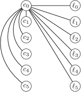
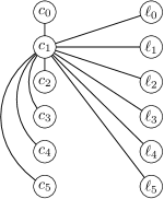
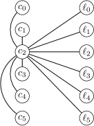
Figure 1: The first three time steps of the temporal graph constructed in the proof of Lemma 3.1 for $r=6$.

Using Lemmas 2.1 and 3.1 we can also show the following.

Corollary 3.2

For every number $k=o(n)$ of agents, there is an infinite family of temporal graphs such that each $n$-vertex temporal graph in the family cannot be explored in $o(n^{2}/k)$ time steps.

Proof. Assume for a contradiction that the corollary does not hold. Then there is a schedule for $k$ agents $A_{1},\ldots,A_{k}$ using $t=o(n^{2}/k)$ time steps to explore the graph described in the proof of Lemma 3.1. We can build a schedule for one agent $A$ as follows: $A$ first behaves as $A_{1}$. After $t$ time steps, $A$ moves to the start vertex (Lemma 2.1) and waits further $O(n)$ time steps until vertex $c_{0}$ becomes the center again. Now $A$ behaves as $A_{2}$—note that the edges are now present in the next $t$ time steps as in the first $t$ time steps. After $tk+O(kn)=o(n^{2})$ time steps, $A$ has explored everything; a contradiction to Lemma 3.1.  $\square$

The underlying graph of the temporal graph constructed in the proof of Lemma 3.1 has maximum degree $|V|-1$. For graphs with maximum degree bounded by $d$, we can show a lower bound of $\Omega(dn)$ on the exploration time. In the following proposition, we present the lower bound construction in a form that we will reuse later in the proof of Theorem 3.7, including the property that a certain subset of the vertices can be explored quickly, which will be needed there. Afterwards, we will state the lower bound in a simpler form as Lemma 3.4.

Proposition 3.3

For every even $d\geq 4$, there is an infinite family of temporal graphs with underlying graphs of maximum degree $d$ that, for every integer $g\geq 1$, contains a temporal graph $\mathcal{G}$ that has $g(d-1)+1=\Theta(gd)$ vertices and requires $\Omega(gd^{2})$ time steps to be explored. That graph contains $g(d/2-1)+1$ vertices, called leaf vertices, such that moving from one of them to any other takes at least $d/2$ time steps. The remaining $gd/2$ vertices are called center vertices and have the property that, starting at an arbitrary vertex of the graph, all center vertices can be explored in at most $g(2d-1)$ time steps.

Proof. Let $g\geq 1$ be given. We construct the temporal graph $\mathcal{G}$ with $g(d-1)+1$ vertices in two steps. First, we take $g$ copies of a temporal graph $\mathcal{G}^{\prime}$, which we connect in the end. $\mathcal{G}^{\prime}$ is the graph with $d$ vertices constructed as in the proof of Lemma 3.1 (by setting the $r$ in Lemma 3.1 to $d/2$). Note that moving from a vertex $\ell_{j}$ in a copy of $\mathcal{G}^{\prime}$ to a vertex $\ell_{k}$ for $k\neq j$ in the same copy of $\mathcal{G}^{\prime}$ requires $\Omega(d)$ time steps.

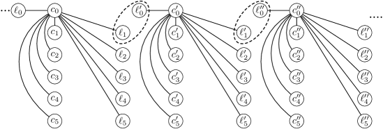
Figure 2: A sketch of the graph of the first time step constructed in the proof of Proposition 3.3. Vertices enclosed by a dashed line are merged to one vertex.

Let $\mathcal{G}_{1},\ldots,\mathcal{G}_{g}$ be the $g$ copies of $\mathcal{G}^{\prime}$. For all $i=1,\ldots,g-1$, connect $\mathcal{G}_{i}$ and $\mathcal{G}_{i+1}$ by merging vertex $\ell_{1}$ of $\mathcal{G}_{i}$ with $\ell_{0}$ of $\mathcal{G}_{i+1}$, i.e., by replacing $\ell_{1}$ and $\ell_{0}$ by a new vertex that has the neighbors of both $\ell_{1}$ and $\ell_{0}$. Let $\mathcal{G}$ be the temporal graph obtained (see Fig. 2 for a sketch of the first time step of $\mathcal{G}$). Note that the underlying graph of $\mathcal{G}$ has maximum degree $d$: The vertices that have been merged have degree $d$, all other vertices $\ell_{j}$ have degree $d/2$, and all vertices $c_{j}$ have degree $d-1$). The vertices $\ell_{j}$ (including the merged vertices) are the leaf vertices, and the vertices $c_{j}$ are the center vertices. By our way of merging, $\mathcal{G}$ is connected at all times as this is true for all copies of $\mathcal{G}^{\prime}$. Furthermore, we observe that $\mathcal{G}$ has $g(d-1)+1$ vertices, because it has $gd/2$ vertices $c_{j}$ and $g\cdot(d/2-1)+1$ vertices $\ell_{j}$, where the ‘+1’ arises from $\ell_{0}$ in $\mathcal{G}_{1}$ and $\ell_{1}$ in $\mathcal{G}_{g}$ not being merged.

Let us consider an exploration schedule of $\mathcal{G}$. By the arguments used in the proof of Lemma 3.1, we can now observe that getting from any $\ell_{i}$ in one copy of $\mathcal{G}^{\prime}$ to a different vertex $\ell_{j}$ in the same or another copy of $\mathcal{G}^{\prime}$ takes at least $d/2$ time steps (in many of these, the agent may not move). As there are at least $g\cdot(d/2-1)=\Omega(gd)$ (recall that $d\geq 4$) such consecutive pairs (ignoring the center vertices) in every exploration schedule of $\mathcal{G}$, we need $\Omega(gd^{2})$ time steps in total.

Finally, consider the exploration of the center vertices. As the graph has $g(d-1)+1$ vertices, we can, starting from an arbitrary vertex at an arbitrary time $t$, move in at most $g(d-1)$ time steps (by Lemma 2.1) to the center vertex in the $g$-th copy of $\mathcal{G}^{\prime}$ that is the center of the star in that copy in time step $t+g(d-1)-1$. From time step $t+g(d-1)$ onward, we can in each step move to the new center of the star in that copy, thus visiting all center vertices in that copy in $d/2-1$ time steps. Then we wait $d/2-1$ time steps until the current vertex is again the center of the star. In that time step we move to the vertex that is the result of merging $\ell_{1}$ in the $(g-1)$-th copy with $\ell_{0}$ in the $g$-th copy, and in the next time step we move from that vertex to the current center in the star of the $(g-1)$-th copy of $\mathcal{G}^{\prime}$. At the start of time step $t+g(d-1)+d$, we are at the center vertex of the $(g-1)$-th copy of $\mathcal{G}^{\prime}$ that has been the center of the star in that copy in the time step just before. Thus, we can repeat the procedure and explore the $(g-1)$-th copy, the $(g-2)$-th copy, etc., in $d$ steps per copy. We complete the exploration of all center vertices in all copies before time step $t+g(d-1)+gd=t+g(2d-1)$.  $\square$

Lemma 3.4

For every $d\geq 2$, there is an infinite family of temporal graphs with underlying graphs of maximum degree at most $d$ that require $\Omega(dn)$ time steps to be explored, where $n$ is the number of vertices of the graph.

Proof. If $d\in\{2,3\}$, take $\mathcal{G}$ to be a static path with $n$ vertices and $n-1$ edges, for any $n\geq 1$. Assume $d\geq 4$. Without loss of generality, we can assume that $d$ is even (otherwise, decrement $d$ by one). The result then follows by Proposition 3.3.  $\square$

In the following, we study the complexity and approximability of the problem of computing an optimal exploration schedule. The next three proofs show NP-hardness results and inapproximability results for TEXP by reductions from the Hamiltonian $s$-$t$ path problem, which is $\mathbf{NP}$-complete even if the input graphs are connected, planar and have maximum degree $3$ as shown by Garey, Johnson, and Tarjan [20]. Moreover, in the proof of Theorem 3.5 we use that their $\mathbf{NP}$-completeness proof shows that the problem remains $\mathbf{NP}$-complete if we further restrict the graphs such that every Hamiltonian path that starts in $s$ (if the graph contains one) must end in $t$. This follows because their reduction from 3SAT to Hamiltonian $s$-$t$ path (via Hamiltonian cycle) only constructs such graphs. (In their words: “a Hamiltonian line must either start at $v_{11}$ and finish at $w_{11}$, or start at $v_{n4}$ and finish at $w_{m6}$.” Hence, if we fix the starting point $s$ to $v_{11}$, then every Hamiltonian path starting in $s$, if one exists, must end in $w_{11}$, and so we can choose $w_{11}$ as $t$.) We call an instance of the Hamiltonian $s$-$t$ path problem with this property a unique destination instance.

Theorem 3.5

TEXP on planar graphs of maximum degree $3$ is $\mathbf{NP}$-hard.

Proof. We give a reduction from the Hamiltonian $s$-$t$ path problem for unique destination instances. Let such an instance be given by a connected planar graph $G^{\prime}=(V^{\prime},E^{\prime})$ with maximum degree $3$ and vertices $s$ and $t$. Take $n^{\prime}=|V^{\prime}|$. Since we can consider $G^{\prime}$ as a temporal graph whose edges always exist, an exploration schedule from $s$ with $n^{\prime}-1$ time steps exists in $G^{\prime}$ if and only if $G^{\prime}$ has a Hamiltonian path from $s$ to $t$. Thus, TEXP on planar graphs of maximum degree $3$ is $\mathbf{NP}$-hard.  $\square$

We remark that temporal graphs whose underlying graph has maximum degree 2 are temporal realizations of paths or cycles. The exploration of temporal realizations of paths is trivial, as all edges of the path must exist in all time steps of every temporal realization since we assume that the graph is connected in each time step. We will show in Theorem 4.7 that temporal realizations of cycles can be explored with arrival time $O(n)$, and an optimal exploration schedule can be computed in polynomial time.

Theorem 3.6

Approximating TEXP with ratio $O(n^{1-\varepsilon})$ is $\mathbf{NP}$-hard for every constant $\varepsilon>0$.

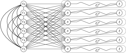
Figure 3: The underlying graph of the temporal graph $\mathcal{H}$ constructed in the proof of Theorem 3.6 where the quick links from $t$ in the $r$th copy of $G^{\prime}$ are not shown.

Proof. Assume we are given an instance $I^{\prime}$ of the Hamiltonian $s$-$t$ path problem consisting of a connected, undirected $n^{\prime}$-vertex graph $G^{\prime}$, a start vertex $s$, and an end vertex $t$. We now construct an instance $I$ of the temporal graph exploration problem as follows: Take the temporal graph $\mathcal{G}$ as constructed in the proof of Lemma 3.1 with $r=(n^{\prime})^{c}$ for a constant $c$ that we will choose later. In addition, replace each $\ell_{i-1}$ by a copy of $G^{\prime}$, called the $i$th copy, for $1\leq i\leq r$. The edges in each copy of $G^{\prime}$ are present in every time step. For all $1\leq i,j\leq r$, the edge $\{c_{j-1},\ell_{i-1}\}$ is replaced by an edge connecting $c_{j-1}$ and vertex $s$ in the $i$th copy. In other words, we identify $s$ in the $i$th copy with $\ell_{i-1}$. Furthermore, we call the vertices $c_{i}$ the center vertices. In addition, we add so-called quick links. Each quick link is an edge that connects the vertex $t$ of the $i$-th copy with the vertex $s$ of the $(i+1)$-th copy only in time step $i\cdot n^{\prime}$, for $1\leq i<r$. There are additional quick links in time step $r\cdot n^{\prime}$ from vertex $t$ in the $r$-th copy to all center vertices. Denote by $\mathcal{H}$ the resulting temporal graph. Its underlying graph is illustrated in Figure 3. Note that $\mathcal{H}$ has $n=r(1+n^{\prime})$ vertices and that $r=\Theta(n^{c/(c+1)})$. Since $\mathcal{G}$ is connected in each time step and each copy of $G^{\prime}$ is connected and present in each time step, $\mathcal{H}$ is also connected in each time step. The start vertex of the exploration is set to be $c_{0}$.

Clearly, if $G^{\prime}$ has a Hamiltonian path from $s$ to $t$, then $\mathcal{H}$ can be explored in $n$ time steps: The agent starts at $c_{0}$ and then explores the first copy of $G^{\prime}$ in $n^{\prime}$ time steps by following the Hamiltonian $s$-$t$-path. The agent arrives at $t$ in the first copy of $G^{\prime}$ at the start of time step $n^{\prime}$, and we can use the unique quick link present in time step $n^{\prime}$ to move to $s$ in the second copy of $G^{\prime}$, etc. After exploring all $r$ copies of $G^{\prime}$, the agent is at $t$ in the $r$-th copy of $G^{\prime}$ at the start of time step $r\cdot n^{\prime}$. Let $c_{i^{\prime}}$ he the vertex that is the center of the star in time step $r\cdot n^{\prime}+1$. The agent moves from $t$ in the $r$-th copy of $G^{\prime}$ to $c_{i^{\prime}}$ via the quick link that is present between these two vertices in time step $r\cdot n^{\prime}$. After that, the agent can explore all remaining center vertices $c_{i^{\prime\prime}}$ in $r$ time steps, i.e., $\mathcal{H}$ can be explored in $n$ time steps—note that $c_{0}$ may be visited twice.

Now assume that $G^{\prime}$ does not have a Hamiltonian $s$-$t$-path. This means that no copy of $G^{\prime}$ can be explored entirely in one visit while using a quick link to enter the copy and another quick link to exit it. If the exploration schedule enters and exits a copy of $G^{\prime}$ via quick links, it must enter that copy at least one more time to explore its remaining vertices. We say that the exploration schedule enters a copy of $G^{\prime}$ via a center vertex if it traverses the edge from a center vertex $c_{i}$ to the $s$ vertex in that copy of $G^{\prime}$, and we say that it exits the copy of $G^{\prime}$ via a center vertex if it traverses the edge from the $s$ vertex in that copy to some center vertex $c_{i}$. Ignoring the last copy of $G^{\prime}$ (in the order in which the copies of $G^{\prime}$ are explored) as well as the copy that is entered or exited via a quick link in time step $r\cdot n^{\prime}$, we therefore have that each of the remaining $r-2$ copies of $G^{\prime}$ is entered or exited (or both) at least once via a center vertex. Whenever a copy of $G^{\prime}$ is exited via a center vertex, the exploration schedule requires $r$ time steps to visit another (or the same) copy of $G^{\prime}$, by the argument in the proof of Lemma 3.1. Whenever a copy of $G^{\prime}$ is entered via a center vertex and is not the first copy visited, the previously visited copy of $G^{\prime}$ must have been exited via a center vertex, except possibly in the case where a quick link from that copy to a center vertex was used. The latter can happen only once, namely at time $r\cdot n^{\prime}$.

Let $k$ be the number of copies of $G^{\prime}$ that are entered via a center vertex, and $l$ the number of copies that are exited via a center vertex. By the discussion above, we have $k+l\geq r-2$ and $l\geq k-2$, which together imply $(l+2)+l\geq r-2$ and thus $l\geq r/2-2$. Perhaps, after the last exit of a copy there is no reenter. Thus, for our $r$ copies of $G^{\prime}$, it happens at least $r/2-3$ times that the exploration schedule moves from a copy of $G^{\prime}$ to another copy of $G^{\prime}$ (or back to the same copy) via a center vertex. As each such move requires at least $r$ time steps, the total number of time steps in the exploration schedule is at least $r(r/2-3)$. So a total of at least $\Omega(r^{2})=\Omega(n^{2c/(c+1)})=\Omega(n^{2-\varepsilon})$ time steps are needed, where $\varepsilon=2/(c+1)$ can be made arbitrarily small by choosing $c$ large enough.

Distinguishing whether $\mathcal{H}$ can be explored in $n$ time steps or whether it requires $\Omega(n^{2-\varepsilon})$ time steps therefore solves the Hamiltonian $s$-$t$-path problem, and the theorem follows.  $\square$

Theorem 3.7

For all $\epsilon,\delta>0$, approximating TEXP with ratio $O(\Delta^{1-\varepsilon})$ is $\mathbf{NP}$-hard even if the underlying graphs have maximum degree at most $\Delta=\Omega(n^{\delta})$ with $n$ being the number of vertices of the temporal graph.

Proof. Choosing our graphs large enough, we assume without loss of generality that $\Delta\geq 8$. Recall that the Hamiltonian $s$-$t$ path problem remains $\mathbf{NP}$-hard if the graphs have maximum degree $3$. Let $I^{\prime}$ be an instance of the Hamiltonian $s$-$t$ path problem consisting of a graph $G^{\prime}=(V^{\prime},E^{\prime})$ with maximum degree $3$ and vertices $s$ and $t$ in $V^{\prime}$ such that $|V^{\prime}|\geq 72$. If $n^{\prime}=|V^{\prime}|$ is not a multiple of $\Delta-4$, then modify $I^{\prime}$ by adding a path of new vertices $v_{1},\ldots,v_{i}$ ($i=-n^{\prime}\,{\mathrm{mod}}\,(\Delta-4)$) and by connecting $v_{i}$ with $t$ and asking for a Hamiltonian $s$-$v_{1}$ path. In this case, we rename the original vertex $t$ to $t^{\prime}$, and rename vertex $v_{1}$ to $t$. Clearly, a solution to the modified instance can be easily turned into a solution of the original instance, and vice versa. Thus, we can assume without loss of generality that $n^{\prime}$ is a multiple of $\Delta-4$ and all vertices except one have degree $\leq 3$ and one vertex $t^{\prime}\neq t$ has degree $\leq 4$.

The idea of the remainder of the proof is to proceed along similar lines as in the proof of Theorem 3.6, but start with the temporal graphs provided by Proposition 3.3 instead of those provided by Lemma 3.1.

First, apply Proposition 3.3 with $d=\Delta-4$ and $g=2(n^{\prime})^{c}/d$ to obtain a temporal graph $\mathcal{G}^{\prime}$, for some integer $c\in I\!\!N$ whose choice will be discussed later. Note that $g$ is an integer as $d=\Delta-4$ divides $n^{\prime}$. $\mathcal{G}^{\prime}$ has $q=gd/2=(n^{\prime})^{c}\geq 72$ center vertices and $r=g(d/2-1)+1=q(d-2)/d+1$ leaf vertices. Now add $r$ disjoint copies of $G^{\prime}$ to $\mathcal{G}^{\prime}$, and identify the vertex $s$ from each copy with a different leaf vertex. The edges in these copies of $G^{\prime}$ are present in every time step. The start vertex of the exploration is set to be an arbitrary center vertex $c_{0}$ that is conneced to some leaf vertex $\ell_{0}$ in the first time step. Order the $r$ copies of $G^{\prime}$ arbitrarily, starting with the copy whose vertex $s$ has been identified with $\ell_{0}$. Denote the copies of $G^{\prime}$ in this order by $G^{\prime}_{0}$, $G^{\prime}_{1}$, …, $G^{\prime}_{r-1}$. For $1\leq i\leq r-1$, add an edge called quick link that connects the vertex $t$ in $G^{\prime}_{i-1}$ with the vertex $s$ in $G^{\prime}_{i}$ and is present only in time step $i\cdot n^{\prime}$. Let $\mathcal{G}$ denote the resulting temporal graph. See Fig. 4 for an illustration of the construction.

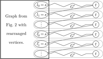
Figure 4: A sketch of the underlying graph constructed in the proof of Theorem 3.7.

The temporal graph $\mathcal{G}$ has $n=q+rn^{\prime}=q(1+n^{\prime}(d-2)/d+n^{\prime})$ vertices, thus $n\leq q(3\cdot q^{1/c})$ and therefore $q\geq(n/3)^{c/(c+1)}\geq n^{c/(c+1)}/3$ $(\star)$. Moreover, it is easy to see that the underlying graph of $\mathcal{G}$ has maximum degree $\Delta$: Center vertices have degree at most $d$. Consider a copy of $G^{\prime}$: Vertex $s$ has at most $d=\Delta-4$ edges to center vertices, one quick link, and $3$ edges to vertices in the same copy; vertex $t^{\prime}$ and $t$ have degree at most 4 due to a possible edge to a new path and a possible quick link, respectively, and all other vertices have degree at most 3.

If $G^{\prime}$ has a Hamiltonian path from $s$ to $t$, then $\mathcal{G}$ can be explored in at most $(r+1)n^{\prime}+4q\leq 4n$ time steps: It takes $n^{\prime}$ time steps to explore the first copy of $G^{\prime}$ (we move from $c_{0}$ to the vertex $s$ in that copy and then follow the Hamiltonian path, reaching the vertex $t$ in that copy in time step $n^{\prime}-1$), then another $n^{\prime}$ time steps to move via the quick link to the second copy and explore it, and so on, with $n^{\prime}$ time steps for each of the $r$ copies of $G^{\prime}$. After $rn^{\prime}$ time steps, we have explored all copies of $G^{\prime}$ and arrived at vertex $t$ in the last copy. Now we move back to the vertex $s$ in that copy using at most $n^{\prime}$ further time steps. It remains to explore the center vertices, which takes at most $g(2d-1)\leq 4q$ time steps by Proposition 3.3.

If $G^{\prime}$ does not have a Hamiltonian $s$-$t$-path, an exploration of the $r$ copies of $G^{\prime}$ in $\mathcal{G}$ must move at least $r/2-3$ times from one copy of $G^{\prime}$ to another via a center vertex, using the same argument as in the proof of Theorem 3.6. By Proposition 3.3, moving from the leaf vertex in one copy to the leaf vertex of another copy via center vertices takes at least $d/2$ time steps. Thus, the exploration of $\mathcal{G}$ takes at least

$$\frac{d}{2}\cdot(r/2-3)\geq\frac{d}{2}\cdot\frac{q(d-2)/d-6}{2}\stackrel{{\scriptstyle d\geq 3,q\geq 72}}{{\geq}}\frac{d}{2}\cdot\frac{q}{8}\stackrel{{\scriptstyle(\star)}}{{\geq}}\frac{d}{48}n^{c/(c+1)}\geq\frac{d}{48}n^{1-\gamma}$$

time steps, where $\gamma>0$ is chosen below and can be made arbitrarily small by making $c$ large enough. Distinguishing whether $\mathcal{G}$ can be explored in at most $4n$ time steps or whether it requires at least $\frac{d}{48}n^{1-\gamma}=\Omega(\Delta n^{1-\gamma})=\Omega(\Delta^{1-\gamma/\delta}n)$ time steps therefore solves the Hamiltonian $s$-$t$-path problem, and the theorem follows by taking $\gamma=\varepsilon\delta$.  $\square$

4 Restricted Underlying Graphs

In Section 3, we showed that arbitrary temporal graphs may require $\Omega(n^{2})$ time steps to be explored and that it is $\mathbf{NP}$-hard to approximate the optimal arrival time of an exploration schedule within $O(n^{1-\varepsilon})$ for every $\varepsilon>0$. This motivates us to consider the case where the underlying graph is from a restricted class of graphs. In particular, the underlying graph of the construction from Lemma 3.1 is dense (it contains $\Omega(n^{2})$ edges) and has large maximum degree. For the case of underlying graphs with degree bound $d$, we could only show that there are graphs that require $\Omega(dn)$ time steps. It is therefore interesting to consider cases of underlying graphs that are sparse, or have bounded degree, or are planar. We consider several such cases in this section. As before, we assume for all temporal graphs under consideration that the graph in each time step is connected and that the lifetime is at least $n^{2}$, where $n$ is the number of nodes of the temporal graph. Furthermore, we still assume that full knowledge about the graphs in all time steps of the given temporal graph is available to an algorithm.

4.1 Lower Bound for Planar Bounded-Degree Graphs

First, we show that even the restriction to underlying graphs that are planar and have bounded degree is not sufficient to ensure the existence of an exploration schedule with a linear number of time steps.

Theorem 4.1

Even if the underlying graph $G=(V,E)$ of a temporal graph $\mathcal{G}$ is planar with maximum degree $4$ and the graph $G_{i}$ in every time step $i\geq 0$ is a simple path, an optimal exploration can take $\Omega(n\log n)$ time steps, where $n=|V|$.

Proof. Without loss of generality, we assume that $n=2^{k}$ for some $k\geq 3$. Consider the following underlying graph $G$: It contains vertices $V_{0}=\{t_{i},b_{i}\mid 0\leq i\leq n/4-1\}$, the edges $\{t_{i},t_{i+1}\},\{b_{i},b_{i+1}\},\{t_{i},b_{i+1}\}$ and $\{b_{i},t_{i+1}\}$ for $0\leq i<n/4-1$, and a path $P$ of $n/2$ additional vertices that connects $t_{0}$ and $b_{0}$—$P$ ensures the connectedness of $\mathcal{G}$. It is not hard to see that $G$ is planar: Arrange the vertices as in Figure 5. For each $0\leq i<n/4-1$, draw the edge $\{b_{i},t_{i+1}\}$ as shown in the figure and the edge $\{t_{i},b_{i+1}\}$ around the outside. We refer to the edges $\{t_{i-1},t_{i}\}$ and $\{b_{i-1},b_{i}\}$ as horizontal edges of column $i$, and the edges $\{t_{i-1},b_{i}\}$ and $\{b_{i-1},t_{i}\}$ as cross edges of column $i$.

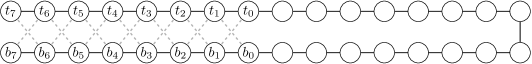
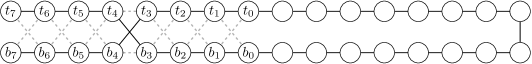
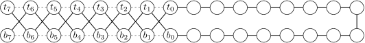
Figure 5: The graphs for different time steps constructed in the proof of Theorem 4.1 for $n=32$. The topmost picture shows the edges present in the first round, the next picture shows the edges present in the second round, etc. The remaining edges of the underlying graph are drawn dashed.

Consider the following temporal realization of $G$: The path $P$ is always present. We divide the time into rounds, each consisting of $n/2$ time steps. The first round consists of the first $n/2$ time steps, etc. For the first round, the graph additionally contains the horizontal edges of all columns. For the next round, the horizontal edges of column $n/8$ are replaced by the cross edges. For the next round, the horizontal edges of columns $n/16$ and $3n/16$ are replaced by the cross edges. Following the same pattern of replacements (each time the horizontal edges of the middle column in each stretch of horizontal edges are replaced by the cross edges), this is repeated for $O(\log n)$ rounds.

For $i\geq 1$, let $G_{i}$ be the graph of the $n/2$ time steps of round $i$ that is induced by $V_{0}$, and let $T_{i}$ and $B_{i}$ denote the vertices of $V_{0}$ that are connected to $t_{0}$ and to $b_{0}$, respectively, in $G_{i}$. Observe that in the $n/2$ time steps of round $i$, an agent can visit either vertices in $T_{i}$ or vertices in $B_{i}$, as it takes more than $n/2$ time steps to travel from $t_{0}$ to $b_{0}$ or vice versa. In particular, after round 1 either $T_{1}$ or $B_{1}$ is entirely unvisited. Let $U_{1}$ be that unvisited set ($U_{1}=T_{1}$ or $U_{1}=B_{1}$). We have $|U_{1}|=n/4$. Observe that in round 2, half the vertices of $U_{1}$ are in $T_{2}$ and the other half in $B_{2}$. If the agent visits vertices of $T_{2}$ in round 2, let $U_{2}=U_{1}\cap B_{2}$; otherwise, let $U_{2}=U_{1}\cap T_{2}$. If we continue in the same way, after $i$ rounds $U_{i}$ is a set containing $|U_{1}|/2^{i-1}=n/2^{i+1}$ unvisited vertices. Thus, no matter what the start position of the agent is, $\Omega(\log n)$ rounds of $\Theta(n)$ time steps each are required until all vertices are visited.  $\square$

4.2 Underlying Graphs with Small Separators

In this section we consider underlying graphs that can be divided into parts in such a way that the parts are small and are connected to the rest of the graph via a small set of so-called boundary vertices. The formal definition is as follows:

Definition 4.2 ($(r,b)$-division)

For positive integers $r$ and $b$ (which might be functions of $n$), an $(r,b)$-division of a graph $G=(V,E)$ with $n$ vertices is given by a separator $S\subseteq V$ and a partition of $G[V\setminus S]$ into $O(n/r)$ (not necessarily connected) components, each associated with a boundary set consisting of vertices from $S$, such that the following properties hold:

1. Each component contains at most $r$ vertices.

2. The boundary set of each component has size at most $b$.

3. The boundary sets of different components may overlap, and the union of the boundary sets of all components is $S$.

4. Every edge of $G$ that has only one endpoint in a component has its other endpoint in the boundary set of that component.

This definition slightly generalizes the $r$-divisions introduced by Frederickson [18] by allowing the choice of the additional parameter $b$.

Theorem 4.3

Every temporal graph whose underlying graph belongs to a class of graphs that have $(r,b)$-divisions can be explored in $O((n^{2}b/r+nrb^{2})\log n)$ time steps.

Proof. We first give an exploration schedule using $b$ agents. The agents explore the $O(n/r)$ components one by one. Consider the exploration of a component $C$ with boundary set $B$. We refer to the vertices in $B$ as boundary vertices. First, we use $O(n)$ time steps to position an agent at each boundary vertex. Now, as the graph is connected in each time step, we know that each vertex $v$ in $C$ is connected to some boundary vertex $w\in B$ in each time step, meaning that there is a path from $v$ to $w$ all of whose internal vertices are in $C$. Therefore, by the pigeonhole principle, for a vertex $v$ in $C$, we have that in every period of $2rb$ time steps, there exists a vertex $w\in B$ such that $v$ is connected to $w$ in at least $2r$ of these $2rb$ time steps. By Lemma 2.1, applied with $H$ as the subgraph of $G$ induced by $w$ and the vertices of $C$, the agent from $w$ can visit $v$ and return to $w$ during these $2r$ time steps, ignoring the other time steps in the period of $2rb$ time steps. Thus, the agents can visit all up to $r$ vertices of $C$ in $2r^{2}b$ time steps. Therefore, the vertices of $C$ and its boundary set are explored in $O(n+r^{2}b)$ time steps, and handling all $O(n/r)$ components one after the other takes $O(n(n+r^{2}b)/r)=O(n^{2}/r+nrb)$ time steps. Finally, we can apply Lemma 2.2 and obtain an exploration schedule with a single agent that uses $O((n^{2}/r+nrb)b\log n)$ time steps.  $\square$

The following lemma will allow us to apply Theorem 4.3 to graphs with bounded treewidth.

Lemma 4.4

Graphs with treewidth at most $k$ admit a $(2\sqrt{n/k},6k)$-division.

Proof. Let $G$ be a graph of treewidth at most $k$. Consider a nice tree decomposition [27, 34] of width $k$ for $G$, i.e., the tree of the tree decomposition is a binary tree and all inner nodes are so-called join nodes, introduce nodes, or forget nodes. The bag of a join node contains the same vertices as the bags of the two children of the join node. Select bags as separators via the following procedure: Visit the bags in a post-order traversal of the tree. Select a bag $B$ as a separator if the number of unmarked vertices in the bag $B$ and in bags below $B$ is at least $\sqrt{n/k}$, or if the number of selected bags that are below $B$ and are not descendants of another selected bag is at least $2$. If a bag $B$ is selected, let the unmarked vertices that are in bags below $B$ but not in $B$ form a new component, and mark all vertices in $B$ and below $B$.

The number of bags selected as separators is $O(\sqrt{nk})$. This can be shown as follows. At any point of the procedure, call a selected bag a topmost bag if it is not a descendant of another selected bag. If a bag is selected because there are at least $\sqrt{n/k}$ unmarked vertices below, the number of topmost bags increases by at most one and $\sqrt{n/k}$ unmarked vertices become marked. This can happen at most $\sqrt{nk}$ times. If a bag is selected because there are two topmost bags below it, the number of topmost bags decreases by one. As the number of topmost bags increases by one at most $\sqrt{nk}$ times, it can also decrease at most $\sqrt{nk}$ times, and hence at most $\sqrt{nk}$ bags are selected because there are two topmost selected bags immediately below them.

As we have a binary tree decomposition, the left and right subtree of a join node whose bag is chosen as separator can have at most $\sqrt{n/k}-1$ unmarked vertices each, so the join node whose bag is chosen as separator could have up to $2\sqrt{n/k}-2$ unmarked vertices below it. When the bag of an introduce or forget node is chosen as separator, there can be at most $\sqrt{n/k}-1$ unmarked vertices below it. As a consequence, the procedure splits the graph into a separator set $S$ (the union of all bags selected as separators) and $O(\sqrt{nk})$ components (that are not necessarily connected) such that each component contains at most $2\sqrt{n/k}-2$ vertices (not counting separators). The boundary set of each component is taken to be the union of the at most three selected bags that separate the component from the rest of the graph: The bag that was selected when the component was formed, and the one or two topmost bags in the subtree below that bag. Thus, the boundary set of each component contains at most $3(k+1)\leq 6k$ vertices.  $\square$

Corollary 4.5

Every temporal graph whose underlying graph has treewidth at most $k$ can be explored in $O(n^{1.5}k^{1.5}\log n)$ time steps.

Proof. By Lemma 4.4, graphs with treewidth at most $k$ admit a $(2\sqrt{n/k},6k)$-division. By Theorem 4.3, applied with $r=2\sqrt{n/k}$ and $b=6k$, the exploration time for temporal graphs whose underlying graph has treewidth at most $k$ is then $O((n^{2}b/r+nrb^{2})\log n)=O(n^{1.5}k^{1.5}\log n)$.  $\square$

Corollary 4.6

Every temporal graph whose underlying graph is planar can be explored in $O(n^{1.8}\log n)$ time steps.

Proof. Using the planar separators introduced by Lipton and Tarjan [28], Frederickson proved that planar graphs with $n$ vertices have $(r,O(\sqrt{r}))$-divisions [18] for every $1\leq r\leq n$. Choosing $r=n^{0.4}$, we can apply Theorem 4.3 with $r=n^{0.4}$ and $b=n^{0.2}$ and obtain that the exploration time for temporal graphs whose underlying graph is planar is $O((n^{2}b/r+nrb^{2})\log n)=O(n^{1.8}\log n)$.  $\square$

4.3 Cycles and Cycles with Chords

Theorem 4.7

Every temporal cycle $\mathcal{C}$ of length $n$ can be explored in at most $2n-2$ time steps, and a schedule using this many time steps can be computed in time linear in the total size of the graphs of the first $2n-2$ time steps, i.e., in $O(n^{2})$ time. If additionally an array $A:\{1,\ldots,2n-2\}\rightarrow E$ is given that stores in $A[t]$ the edge that is missing in time step $t$, if any, then the running-time can be improved to $O(n)$. Moreover, an optimal schedule for exploring a temporal cycle can be computed in polynomial time.

Proof. We start by showing that $2n-2$ time steps suffice to explore every temporal cycle of length $n$. The exploration schedule is constructed in two phases. In the first phase, our goal is to distribute $n$ virtual agents over the whole cycle. In detail, move $n$ virtual agents from the start vertex to all vertices of the cycle such that one virtual agent is on each vertex, its virtual start vertex. By Lemma 2.1, this can be done in $n-1$ time steps.

In the second phase, which follows the first phase, all virtual agents move in clockwise direction in each time step. Whenever a virtual agent cannot move due to a temporal missing edge, that virtual agent disappears. Note that a temporal missing edge can cause the disappearance of at most one virtual agent in each time step. Therefore, at least one virtual agent remains after $n-1$ time steps in the second phase. The exploration schedule of that virtual agent has explored the whole temporal cycle in at most $2n-2$ time steps.

We can compute a schedule using $2n-2$ time steps efficiently as follows. Consider the second phase and maintain the set of agents that have not yet disappeared. For each time step $i=n,\ldots,2n-2$, spend $O(1)$ time to determine the agent that starts $i-n+1$ vertices counterclockwise to the missing edge, i.e., determine the agent that disappears, if any. Finally, take one of the agents that remains in the set and compute a schedule for it to reach its virtual start vertex during the first phase. If we spend $O(n^{2})$ time to iterate over the graphs of the first $2n$ time steps and build the array $A$, then it is easy to see that the remaining computation can be done in $O(n)$ time.

Finally, we show how to compute an optimal exploration schedule in polynomial time. By shortcutting backward and forward moves of the agents such that no vertices are skipped completely, every optimal schedule can be converted into one with the same arrival time that falls into one of these types: move clockwise around the cycle; move counter-clockwise around the cycle; move clockwise to some vertex $v$, then counter-clockwise until the cycle is explored; move counter-clockwise to some vertex $w$, then clockwise until the cycle is explored. The types can be enumerated in polynomial time, and the optimal schedule for each type can be calculated in a greedy way. The best of these schedules can then be output as the optimal exploration schedule for the given temporal cycle.  $\square$

Observation 4.8

For every $n\geq 3$, there is a temporal cycle of length $n$ in which the optimal exploration requires at least $2n-3$ time steps.

Proof. Assume that $u,v,w$ are three consecutive vertices in this order of the cycle and the agent is initially at $u$. Let the edge $\{u,v\}$ be absent for the first $n-2$ time steps, and let the edge $\{v,w\}$ be absent in all time steps after that. The agent cannot traverse the edge $\{v,w\}$ as it can reach neither $v$ nor $w$ before the edge disappears forever. So, the only two candidates for an optimal exploration schedule are the following: We can either wait at $u$ until $\{u,v\}$ is available ($n-2$ time steps), move to $v$ ($1$ time step) and then walk to $w$ ($n-1$ time steps), giving a total of $2n-2$ time steps, or walk to $w$ in $n-2$ time steps and then from $w$ to $v$ in $n-1$ time steps, giving a total of $2n-3$ time steps.  $\square$

A graph is a tree of rings if it is connected and all its blocks are cycles. By Lemma 2.7, it follows that temporal graphs whose underlying graph $G$ is a tree of rings with $n$ nodes can be explored in $O(n)$ time steps provided that each cycle of $G$ contains at most a constant number of cut nodes of $G$.

Next, we show that the addition of a single chord to a cycle does not destroy the property of admitting an exploration schedule with $O(n)$ time steps.

Theorem 4.9

A temporal cycle of length $n$ with one chord can be explored in $O(n)$ time.

Proof. Let the left and right cycle be the two cycles that contain the chord. Check how often the chord is present in the first $7n$ time steps. If the chord is present in at least $5n$ time steps, use $2n$ of these to explore the (left or right) cycle in which the start node is contained (which is possible by Theorem 4.7), $n$ time steps to move to the other cycle, and $2n$ time steps to explore that cycle. Otherwise, there are at least $2n$ time steps in which the chord is absent and the remaining graph is a cycle instance. The cycle can be explored in these time steps.  $\square$

We conjecture that Theorem 4.9 can be extended to $O(1)$ chords.

4.4 The $2\times n$ Grid

In this section, we consider temporal graphs whose underlying graph is a grid with $2$ rows and $n$ columns.

Theorem 4.10

Every temporal $2\times n$ grid can be explored in $O(n\log n)$ time steps with $4\log n$ agents.

Proof. We show a slightly more general statement. We show that, if we are given an underlying graph $G^{\prime}$ being a grid of size $2\times n^{\prime}$ and a subgrid $G^{\prime\prime}$ of size $2\times n^{\prime\prime}$ of $G^{\prime}$ such that each pair of vertices in $G^{\prime\prime}$ is connected in $G^{\prime}$ in each time step (i.e., for every two vertices $u,v$ in $G^{\prime\prime}$, the graph contains a path from $u$ to $v$ in $G^{\prime}$ in each time step), then $4\log n^{\prime}$ agents initially on some vertices of $G^{\prime\prime}$ can explore $G^{\prime\prime}$ in $T(n^{\prime})=O(n^{\prime}\log n^{\prime})$ time. The theorem follows by taking $G^{\prime}=G^{\prime\prime}=G$. See also Figure 6.

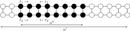
Figure 6: The situation as described in the proof of Theorem 4.10. A grid $G^{\prime}$ with a subgrid $G^{\prime\prime}$ (indicated by the black vertices) and the initial position of the agents to explore the left half of $G^{\prime\prime}$.

We start with exploring the left half $H^{\prime}$ of $G^{\prime\prime}$. The idea is to move $4$ agents to the corners of $H^{\prime}$, one to each corner, and all remaining $4(\log n^{\prime})-4$ agents to a suitable middle location of $H^{\prime}$—specified below—using the first $2n^{\prime}$ time steps. This is possible by Lemma 2.1. For the next $T(n^{\prime}/2)+n^{\prime}/2$ time steps, in each time step where it is possible, we move the $2$ agents $\ell_{1}$ and $\ell_{2}$ on the left corners of $H^{\prime}$ in parallel to the right using only horizontal edges. Similarly, we move the $2$ agents $r_{1}$ and $r_{2}$ on the right corners to the left in parallel. Let $i$ and $j$ be the number of actual moves (i.e., the number of time steps during which the agents could move) of $\ell_{1}$ and $r_{1}$, respectively. The middle location is any position between the final position of $\ell_{1}$ and $\ell_{2}$ on the left and the final position of $r_{1}$ and $r_{2}$ on the right. If the agents on the left and on the right meet, they stop moving and $H^{\prime}$ is explored. In particular, if $H^{\prime}$ is a $2\times 1$ grid, $\ell_{1}$ and $r_{1}$ (as well as $\ell_{2}$ and $r_{2}$) are at the same vertex, i.e., we can stop immediately and $T(1)=O(1)$. Otherwise, we have $i+j<n^{\prime\prime}/2\leq n^{\prime}/2$ and in the same $T(n^{\prime}/2)+n^{\prime}/2$ time steps where the $4$ agents try to move, we explore recursively the subgrid $H^{\prime\prime}$ of $H^{\prime}$ consisting of the columns that are not visited by the $4$ corner agents. More precisely, there are at least $T(n^{\prime}/2)+n^{\prime}/2-i-j\geq T(n^{\prime}/2)$ time steps in which neither the $2$ agents $\ell_{1}$ and $\ell_{2}$ nor the $2$ agents $r_{1}$ and $r_{2}$ move, and each pair of vertices of $H^{\prime\prime}$ is connected in $H^{\prime}$ in each of these time steps. Therefore, the agents starting in the middle location can explore $H^{\prime\prime}$ in $T(n^{\prime}/2)$ of those time steps. Consequently, after the first $2n^{\prime}$ time steps to place the agents, the next $T(n^{\prime}/2)+n^{\prime}/2$ time steps are enough to explore $H^{\prime}$.

We subsequently explore the right half in the same way. The total time to explore $G^{\prime\prime}$ is $T(n^{\prime})\leq 2(2n^{\prime}+T(n^{\prime}/2)+n^{\prime}/2)=O(n^{\prime}\log n^{\prime})$.  $\square$

Using Lemma 2.2, we can reduce the number of agents to one.

Corollary 4.11

A temporal $2\times n$ grid can be explored in $O(n\log^{3}n)$ time steps by one agent.

Let $H_{n}$ be the graph that consists of a path with $n-1$ vertices and one additional vertex that is adjacent to all vertices on the path. Note that $H_{n}$ can be obtained from the $2\times(n-1)$ grid using $n-2$ edge contractions. Therefore, Corollary 2.6 implies that every temporal $H_{n}$ can be explored in $O(n\log^{3}n)$ time steps by one agent.

5 Temporal Graphs with Regularly Present Edges

We say that a temporal graph has regularly present edges if for every edge $e$ there is a constant integer $I_{e}$ with the property that, whenever $e$ is absent from the temporal graph, the number of consecutive time steps during which $e$ is absent is strictly less than $I_{e}$. In other words, if edge $e$ is not present in some time step $t$, then the first time step after $t$ when $e$ is present again is no later than time step $t+I_{e}-1$. Moreover, in contrast to the rest of the paper, in this and the following section, we drop the assumption that we know the schedule of the existing edges in advance. In other words, for the rest of the paper, we consider an online problem where the algorithm only knows $I_{e}$ for each edge $e$, but has no advance information in which time step an edge is present. In each time step $i$, the algorithm has to decide whether to stay at its current vertex $v$ or move to a neighbor of $v$ in the current graph knowing only the graphs of all time steps up to $i$. We also drop the connectedness assumption in this and the following section. In this section, we only require that there is a constant $c\geq 1$ such that, over every cut $S$, it is guaranteed that there is an edge on average at least once every $c$ time steps, i.e., $\sum_{e:|e\cap S|=1}1/I_{e}\geq 1/c$ or, equivalently, $\sum_{e:|e\cap S|=1}c/I_{e}\geq 1$.

Theorem 5.1

A temporal graph $\mathcal{G}$ with regularly present edges whose underlying graph has $n$ vertices and $m$ edges can be explored online in $O(m)$ time steps.

Proof.For each $I_{e}$, let $J_{e}$ be the largest power of $2$ with $J_{e}\leq I_{e}$. Calculate a minimum spanning tree $T$ of the underlying graph with respect to edge weights $J_{e}$. Explore the graph by following an Euler tour of $T$ (if the next edge of the tour is not present in the current time step, simply wait at the current vertex until the edge becomes available). Moving over an edge $e$ takes at most $I_{e}\leq 2J_{e}$ time steps, so the total exploration takes at most $4\sum_{e\in T}J_{e}$ time steps.

We next show that $\sum_{e\in T}J_{e}=O(m)$. The idea is, for each edge $e$ of $T$, to split $J_{e}$ into several charges and to distribute these charges to several edges such that, afterwards, one can show that the sum of the charges distributed to each edge is $O(1)$. Consider any $k\geq 0$ such that $T$ contains at least one edge $e$ with $J_{e}=2^{k}$. Consider the connected components $C_{1},\ldots,C_{r_{k}}$ of $T\setminus\{e\in T\mid J_{e}=2^{k}\}$. Observe that every edge of $\mathcal{G}$ leaving a component $C_{i}$ (i.e., with one endpoint in $C_{i}$) must have weight at least $2^{k}$ since, otherwise, the tree would not contain $e$, but an edge with smaller weight than $e$. Let $E_{i}$ be the set of edges of the underlying graph of $\mathcal{G}$ that leave $C_{i}$. Since $\sum_{e\in E_{i}}c/I_{e}\geq 1$, $\sum_{e\in E_{i}}c/J_{e}\geq 1$. Assign a charge of $c2^{k}/J_{e}$ to each $e\in E_{i}$. The total charge that $C_{i}$ assigns to $E_{i}$ is $\sum_{e\in E_{i}}c2^{k}/J_{e}=2^{k}\sum_{e\in E_{i}}c/J_{e}\geq 2^{k}$. Since an edge receives the charge $c2^{k}/J_{e}$ from at most two components $C_{i}$, no edge receives more than $2c2^{k}/J_{e}$ of charge for every fixed $k$.

The total weight of edges of weight $2^{k}$ in $T$ is $2^{k}(r_{k}-1)$. Each of the $r_{k}$ components assigns a charge of at least $2^{k}$ to edges, so the total charge of the $r_{k}$ components is greater than the total cost of edges of weight $2^{k}$ in $T$.

To bound the total charge that an edge $e$ of $G$ can receive, let the weight of $e$ be $J_{e}=2^{j}$. For $k>j$, $e$ does not receive any charge. For each $0\leq k\leq j$, $e$ receives charge at most $2c2^{k}/2^{j}$. The total charge received by $e$ is then at most $\sum_{k=0}^{j}\frac{2c2^{k}}{2^{j}}\leq\frac{2c2^{j+1}}{2^{j}}=4c$.

So we have that all the weight of $T$ is charged to edges of $G$, and no edge of $G$ receives more than $4c$ of charge. As $G$ has $m$ edges, the total charge is at most $4cm=O(m)$, and hence the weight of $T$ is $O(m)$.  $\square$

6 Random Temporal Graphs

Let $G=(V,E)$ be a given graph with $n$ vertices and $m$ edges. As in the previous section, we do not assume that we know the schedule of the edges. Instead, we now know the probabilities $p_{e}$ for all $e\in E$ such that each edge $e$ exists in every time step with probability $p_{e}$. We assume that the probabilities of two edges are independent. $G$ is not necessarily connected in each time step. In order to guarantee that exploration is always possible, we make the following assumption that replaces the connectedness condition in every time step by a probabilistic analogue: We require that, for every cut, the number of edges crossing the cut is at least some constant in expectation in every time step. More precisely, we now assume that the total sum of the probabilities of the edges over each cut of $G$ is greater or equal than $1/c$ for some arbitrary constant $c\geq 1$. In particular, this implies that $m\geq n-1$.

Theorem 6.1

Let $G$ be a random graph with $n$ vertices and $m$ edges where each edge $e$ exists with probability $p_{e}$ and where the total sum of the probabilities of the edges over each cut of $G$ is greater or equal than some constant. Then, for every constant $d\geq 1$ we can find an online exploration schedule of an agent that uses only $O(m\log n)$ time steps with probability $1-1/n^{d}$. The exploration schedule traverses an Euler tour of a minimum spanning tree of $G$ with respect to edge weights $I_{e}=1/p_{e}$.

Proof. To explore $G$, we first determine a spanning tree $T$ as in the previous section after setting the weight of $e$ to $I_{e}=1/p_{e}$. Then we explore $G$ by an Euler Tour of $T$. Let $\ell\geq 2$ be some positive number that we fix later. The number of time steps an edge $e$ is present in an interval of $t=\lceil\ell\cdot I_{e}\rceil$ time steps is a random variable $X_{e}$ with $Pr[X_{e}<1]=(1-p_{e})^{t}\leq(1-p_{e})^{\ell/p_{e}}\leq\exp(-\ell)$. Intuitively speaking, with increasing $\ell$, the probability that $e$ is not present in any of $t$ consecutive time steps drops exponentially. Since the Euler tour visits each edge of $T$ twice, the probability that the total exploration takes more than $2\sum_{e\in T}\lceil\ell\cdot I_{e}\rceil\leq 2n+2\sum_{e\in T}\ell\cdot I_{e}$ time steps can be upper bounded by $2\sum_{e\in T}\exp(-\ell)\leq 2n\exp(-\ell)$. By choosing $\ell=3d\cdot\ln n$ for some constant $d\geq 1$, this bound is $\leq 1/n^{d}$. Thus, with high probability (with probability $1-1/n^{d}$), we can explore $G$ in $\tau=\lceil 2n+2\sum_{e\in T}\ell\cdot I_{e}\rceil\leq\lceil 2n+4\ell\sum_{e\in T}J_{e}\rceil=O(m\log n)$ time steps as shown in the proof of Theorem 5.1, where $\sum_{e:|e\cap S|=1}c/I_{e}=\sum_{e:|e\cap S|=1}c\cdot p_{e}\geq 1$ for each cut $S\subseteq V$ of $G$ follows from the fact that the total sum of the probabilities of the edges over the cut $S$ is greater or equal than $1/c$.  $\square$

7 Application: Gossiping Problem

In this section we consider a distributed computing problem in a network of processors where the presence of links in each time step is determined in the same way as in the random temporal graphs considered in Section 6. Formally, the problem and the model of computation are defined as follows. Throughout this section, we refer to time steps as rounds, as is common in distributed computing.

First, we define the model of distributed computing that we consider.

Definition 7.1 (Model of Distributed Computing)

Consider the following model of distributed computing in random temporal graphs: Let $G$ be a connected graph with $n$ vertices and $m$ edges, representing a communication network where each vertex is a processor. In each round, each edge $e$ of $G$ is present with an independent probability $p_{e}$. The graph $G$ represents the underlying graph of a random temporal graph, and the edge probabilities $p_{e}$ describe the temporal realization of $G$. For some arbitrary constant $c\geq 1$, the sum of the probabilities $p_{e}$ of the edges $e$ over each cut of $G$ must be at least $1/c$. Each vertex has a unique id and knows the following at the start of the computation:

• its own id

• $n$ and $m$,

• the moment in time when the distributed computation starts,

• for each edge $e$ that is incident with the vertex, the id of the opposite endpoint and the probability $p_{e}$ of $e$ to exist in a time step.

The computation proceeds in synchronous rounds. In every round, each vertex can do an arbitrary amount of local computation and send one message of arbitrary size (consisting possibly of all information known to the vertex) to one of its neighbors. A message from a vertex to a neighbor can only be received if the edge between the two vertices exists in that round, and the sender can only detect the presence of the edge by a successful message delivery. Both successful and unsuccessful message transmissions are counted in the total number of messages.

Now we define the gossiping problem that we want to solve.

Definition 7.2 (Gossiping   Problem   in   Random   Temporal   Graphs)

Consider the model of distributed computing in random temporal graphs of Definition 7.1. At the start of the computation, each vertex (processor) additionally has an initial value. The goal of the gossiping problem in random temporal graphs is to distribute the initial value of each vertex to all other vertices.

Our aim is to present a distributed algorithm to solve the gossiping problem in random temporal graphs while sending only a small total number of messages over the edges of $G$. Since we later want to use $4\lceil\log n\rceil\leq n$, we assume that $n\geq 20$ in the remainder of this section.

The basic idea of our algorithm is to first determine a minimum spanning tree $T$ of $G$ with respect to edge weights defined by setting the weight of each edge $e$ to $I_{e}=1/p_{e}$ (as in the proof of Theorem 6.1), and then to use two traversals of an Euler tour of $T$ to distribute the value of each processor to all other processors. Once the minimum spanning tree $T$ has been constructed, the same tree can be re-used to solve further gossiping problems without recomputing the tree.

First, we adapt the minimum-spanning-tree algorithm of Gallager, Humblet, and Spira [19] to our model of distributed computing in random temporal graphs.

Lemma 7.3

In the model of distributed computing of Definition 7.1, a minimum spanning tree $T$ of $G$ with respect to edge weights set to $I_{e}=1/p_{e}$ for all edges $e$ of $G$ can be built using $O(m\log^{2}n)$ messages with probability at least $1-1/n^{d-1}$.

Proof. We compute $T$ in phases similar to Kruskal’s algorithm, with growing connected components distributed over the whole graph. Moreover, each phase is divided into four subphases; each runs for exactly $\tau$ rounds where $\tau=O(m\log n)$ is the integer defined in the proof of Theorem 6.1. Let us assume that at the beginning of each phase, all vertices of each component know the set of vertex ids of all vertices of the component, and hence also the minimal id of a vertex belonging to the component. In the following, we describe our algorithm by tokens walking around in the graph. Whenever a token moves from one vertex $u$ to another vertex $v$, a message is sent from $u$ to $v$ until the edge $\{u,v\}$ is present in $G$.

Each phase consists of several subphases, which itself consist of several rounds. In the first subphase, each vertex first identifies its incident edge of minimal weight leaving the component (a vertex can determine whether an incident edge leaves its component because it knows the set of vertex ids of its component as well as the vertex id of the other endpoint of the edge), and the vertex of minimal id in each component starts a token that walks around the so far constructed minimum spanning tree twice; first to collect and then to distribute the information on these edges. Afterwards, each vertex in every component knows the edge of minimal weight leaving its component—to make the weight unique, incorporate the vertex ids in the weights. Let us call these edges the new edges (of the final minimum spanning tree). Moreover, for each component $C$ and the new edge $e_{C}$ chosen by the component, define the vertex in the component incident to the new edge as the start vertex $s_{C}$ of the component.

In a second subphase, the start vertex $s_{C}$ of each component $C$ informs the opposite vertex of the new edge $e_{C}$ that it is incident to a new edge, which will connect both components soon. This can be done by sending a message from each start vertex over its incident new edge.

In a third subphase, each component $C$ starts a new token from $s_{C}$ walking around the minimum spanning tree of the component. Whenever the token visits a vertex $v$ that is incident to a new edge $e_{C^{\prime}}\neq e_{C}$ of another component $C^{\prime}$, the token of $C$ waits for a message over $e_{C^{\prime}}$ from the token walking around in $C^{\prime}$. To be more precise, the token for $C$ waits for a message for each new edge $e\neq e_{C}$ incident to $v$. (Possibly, this already happened before the token reaches $v$. Then the token can continue immediately.) Finally, after the token returned to its start vertex $v$, i.e, after visiting all vertices of the old component $C$ and after receiving a message over all incident new edges $e\neq e_{C}$, a message is sent over $e_{C}$ with all ids known by $C$’s token.

Assume that the tokens above collect all ids of both, the visited vertices and the ids received from other tokens sent by their messages over the new edges. We next want to show that there is then a token at the end of the subphase that knows all vertex ids of the new component. For the analysis, let us merge each component to one vertex and direct the new edges in the direction in which the message is sent. (Since over the final edge messages are sent simultaneously in both directions, the endpoints of the edge must agree to ignore one of the two messages.) In this way we obtain a rooted intree. It is not hard to see that the root of the tree is exactly the component whose token finishes its travel last and knows all vertex ids.

In a fourth subphase, these last finished tokens (one for each new component) can travel the spanning tree of the new component to inform all vertices about the set of vertex ids of the new component, and hence also about the new vertex with minimal id. This finishes the current phase and the next phase can start.

To bound the number of messages sent in one phase observe that the total number of messages in each subphase is bounded by a constant factor times the number of messages of an Euler tour of the final minimum spanning tree. This is because we only send messages over edges that are also used by the Euler tour and because, since the probabilities of two edges are independent, it makes no difference in which order the messages are sent (even parallel sending is possible). Moreover, since the number of components halves in each phase, there are $\lceil\log n\rceil$ phases. Thus by Theorem 6.1, we can build $T$ with $O(m\log^{2}n)$ messages with probability $\geq 1-4\lceil\log n\rceil/n^{d}\geq 1-1/n^{d-1}$.  $\square$

We are now ready to prove the main theorem of this section.

Theorem 7.4

Let $d\geq 1$ be any constant. Consider the model of distributed computing of Definition 7.1. After building a minimum spanning tree using $O(m\log^{2}n)$ messages with probability at least $1-1/n^{d-1}$, we can solve instances of the gossiping problem on $G$ with $O(m\log n)$ messages per instance with probability at least $1-2/n^{d}$.

Proof. The message bound for constructing the minimum spanning tree is given by Lemma 7.3. Once the minimum spanning tree has been constructed, we can solve the gossiping problem as follows. Starting from the vertex of minimal id we can send a message collecting all initial values along the Euler tour twice, in a first traversal to collect all initial values and in a second traversal to distribute them. By Theorem 6.1, we can run each traversal with $O(m\log n)$ messages with probability $\geq 1-1/n^{d}$.  $\square$

We finally want to remark that the number of successfully transmitted messages for the initialization (minimum spanning tree computation) and for solving the gossiping problem is $O(n\log n)$ and $O(n)$, respectively.

8 Conclusion

Even though the literature on temporal graphs has grown substantially in recent years, the study of temporal graphs is still in its infancy, and we do not yet have intuition and a range of techniques comparable to what has been developed over many years for static graphs. Even seemingly simple tasks such as constructing temporal graphs (possibly with an underlying graph from a given family) that cannot be explored quickly is surprisingly difficult. We hope that the methods used in this paper to prove results for temporal graphs, e.g., the general conversion of multi-agent solutions to single-agent solutions, contribute to the formation of a growing toolbox for dealing with temporal graphs.

Our results directly suggest a number of questions for future work. In particular, deriving tight bounds on the largest number of time steps required to explore a temporal graph whose underlying graph is an $m\times n$ grid, a bounded degree graph, or a planar graph would be interesting. We have given a lower bound of $\Omega(n\log n)$ time steps for a specific family of temporal graphs whose underlying graph is planar and has bounded degree, but the upper bounds we have are only $O(n^{1.8}\log n)$ time steps for underlying planar graphs and $O(n^{1.75})$ time steps for the case where the graph in each time step has bounded degree [15]. Closing this gap would be a worthwhile research direction. It would also be interesting to study the approximability of TEXP for restricted underlying graphs, and to identify further cases of underlying graphs where the temporal exploration problem can be solved optimally in polynomial time.

References

- Ajtai et al. [1982] Miklós Ajtai, János Komlós, and Endre Szemerédi. Largest random component of a k-cube. Combinatorica, 2(1):1–7, 1982. doi:10.1007/BF02579276.
- Avin et al. [2018] Chen Avin, Michal Koucký, and Zvi Lotker. Cover time and mixing time of random walks on dynamic graphs. Random Struct. Algorithms, 52(4):576–596, 2018. doi:10.1002/rsa.20752.
- Bender et al. [1998] Michael A. Bender, Antonio Fernández, Dana Ron, Amit Sahai, and Salil Vadhan. The power of a pebble: Exploring and mapping directed graphs. In Proc. 30th Annual ACM Symposium on Theory of Computing (STOC 1998), pages 269–278, New York, NY, USA, 1998. ACM. doi:10.1145/276698.276759.
- Berman [1996] Kenneth A. Berman. Vulnerability of scheduled networks and a generalization of Menger’s theorem. Networks, 28(3):125–134, 1996. doi:10.1002/(SICI)1097-0037(199610)28:3<125::AID-NET1>3.0.CO;2-P.
- Bermond et al. [1995] Jean-Claude Bermond, Luisa Gargano, Adele A. Rescigno, and Ugo Vaccaro. Fast gossiping by short messages. In Proc. 22nd International Colloquium on Automata, Languages and Programming (ICALP95), volume 944 of LNCS, pages 135–146. Springer, 1995. doi:10.1007/3-540-60084-1_69.
- Biswas et al. [2015] Sudip Biswas, Arnab Ganguly, and Rahul Shah. Restricted shortest path in temporal graphs. In Proc. 26th International Conference on Database and Expert Systems Applications (DEXA 2015), Part I, volume 9261 of LNCS, pages 13–27. Springer, 2015. doi:10.1007/978-3-319-22849-5_2.
- Brodén et al. [2004] Björn Brodén, Mikael Hammar, and Bengt J. Nilsson. Online and offline algorithms for the time-dependent TSP with time zones. Algorithmica, 39(4):299–319, 2004. doi:10.1007/s00453-004-1088-z.
- Bui-Xuan et al. [2003] Binh-Minh Bui-Xuan, Afonso Ferreira, and Aubin Jarry. Computing shortest, fastest, and foremost journeys in dynamic networks. Int. J. Found. Comput. Sci., 14(2):267–285, 2003. doi:10.1142/S0129054103001728.
- Casteigts et al. [2012] Arnaud Casteigts, Paola Flocchini, Walter Quattrociocchi, and Nicola Santoro. Time-varying graphs and dynamic networks. IJPEDS, 27(5):387–408, 2012. doi:10.1080/17445760.2012.668546.
- Casteigts et al. [2014] Arnaud Casteigts, Paola Flocchini, Bernard Mans, and Nicola Santoro. Measuring temporal lags in delay-tolerant networks. IEEE Trans. Computers, 63(2):397–410, 2014. doi:10.1109/TC.2012.208.
- Chlebus and Kowalski [2002] Bogdan S. Chlebus and Dariusz R. Kowalski. Gossiping to reach consensus. In Proc. 14th Annual ACM Symposium on Parallelism in Algorithms and Architectures (SPAA 2002), pages 220–229. ACM, 2002. doi:10.1145/564870.564908.
- Di Luna et al. [2016] Giuseppe Antonio Di Luna, Stefan Dobrev, Paola Flocchini, and Nicola Santoro. Live exploration of dynamic rings. In Proceedings of the 36th IEEE International Conference on Distributed Computing Systems (ICDCS 2016), pages 570–579. IEEE Computer Society, 2016. doi:10.1109/ICDCS.2016.59.
- Diestel [2010] Reinhard Diestel. Graph Theory. Number 173 in Graduate Texts in Mathematics. Springer, 4th edition, 2010.
- Erlebach et al. [2015] Thomas Erlebach, Michael Hoffmann, and Frank Kammer. On temporal graph exploration. In Magnús M. Halldórsson, Kazuo Iwama, Naoki Kobayashi, and Bettina Speckmann, editors, 42nd International Colloquium on Automata, Languages, and Programming (ICALP 2015), volume 9134 of Lecture Notes in Computer Science, pages 444–455. Springer, 2015. doi:10.1007/978-3-662-47672-7_36.
- Erlebach et al. [2019] Thomas Erlebach, Frank Kammer, Kelin Luo, Andrej Sajenko, and Jakob T. Spooner. Two moves per time step make a difference. In Christel Baier, Ioannis Chatzigiannakis, Paola Flocchini, and Stefano Leonardi, editors, 46th International Colloquium on Automata, Languages, and Programming (ICALP 2019), volume 132 of LIPIcs, pages 141:1–141:14. Schloss Dagstuhl - Leibniz-Zentrum für Informatik, 2019. doi:10.4230/LIPIcs.ICALP.2019.141.
- Erlebach et al. [2021] Thomas Erlebach, Michael Hoffmann, and Frank Kammer. On temporal graph exploration. Journal of Computer and System Sciences, 119:1–18, 2021. doi:https://doi.org/10.1016/j.jcss.2021.01.005.
- Flocchini et al. [2009] Paola Flocchini, Bernard Mans, and Nicola Santoro. Exploration of periodically varying graphs. In Proc. 20th International Symposium on Algorithms and Computation (ISAAC 2009), volume 5878 of LNCS, pages 534–543. Springer, 2009. doi:10.1007/978-3-642-10631-6_55.
- Frederickson [1987] Greg N. Frederickson. Fast algorithms for shortest paths in planar graphs, with applications. SIAM J. Comput., 16(6):1004–1022, 1987. doi:10.1137/0216064.
- Gallager et al. [1983] Robert G. Gallager, Pierre A. Humblet, and Philip M. Spira. A distributed algorithm for minimum-weight spanning trees. ACM Trans. Program. Lang. Syst., 5(1):66–77, 1983. doi:10.1145/357195.357200.
- Garey et al. [1976] M. R. Garey, David S. Johnson, and Robert Endre Tarjan. The planar hamiltonian circuit problem is NP-complete. SIAM J. Comput., 5(4):704–714, 1976. doi:10.1137/0205049.
- Hromkovic et al. [2005] Juraj Hromkovic, Ralf Klasing, Andrzej Pelc, Peter Ruzicka, and Walter Unger. Dissemination of Information in Communication Networks - Broadcasting, Gossiping, Leader Election, and Fault-Tolerance. Texts in Theoretical Computer Science. An EATCS Series. Springer, 2005. ISBN 978-3-540-00846-0. doi:10.1007/b137871.
- Ilcinkas and Wade [2018] David Ilcinkas and Ahmed Mouhamadou Wade. Exploration of the t-interval-connected dynamic graphs: the case of the ring. Theory of Computing Systems, 62(5):1144–1160, 2018. doi:10.1007/s00224-017-9796-3.
- Ilcinkas et al. [2014] David Ilcinkas, Ralf Klasing, and Ahmed Mouhamadou Wade. Exploration of constantly connected dynamic graphs based on cactuses. In Proceedings of the 21st International Colloquium on Structural Information and Communication Complexity (SIROCCO 2014), volume 8576 of LNCS, pages 250–262. Springer, 2014. doi:10.1007/978-3-319-09620-9_20.
- Karlin et al. [1994] Anna R. Karlin, Greg Nelson, and Hisao Tamaki. On the fault tolerance of the butterfly. In Proc. 26th Annual ACM Symposium on Theory of Computing (STOC 1994), pages 125–133. ACM, 1994. doi:10.1145/195058.195117.
- Kempe et al. [2002] David Kempe, Jon M. Kleinberg, and Amit Kumar. Connectivity and inference problems for temporal networks. J. Comput. Syst. Sci., 64(4):820–842, 2002. doi:10.1006/jcss.2002.1829.
- Kesten [1980] Harry Kesten. The critical probability of bond percolation on the square lattice equals . Comm. Math. Phys., 74(1):41–59, 1980.
- Kloks [1994] Ton Kloks. Treewidth, Computations and Approximations, volume 842 of LNCS. Springer, 1994. ISBN 3-540-58356-4. doi:10.1007/BFb0045375.
- Lipton and Tarjan [1979] Richard J. Lipton and Robert Endre Tarjan. A separator theorem for planar graphs. SIAM J. Appl. Math., 36(2):177–189, 1979.
- Liu and Wu [2009] Cong Liu and Jie Wu. Scalable routing in cyclic mobile networks. IEEE Trans. Parallel Distrib. Syst., 20(9):1325–1338, 2009. doi:10.1109/TPDS.2008.218.
- Lynch [1996] Nancy A. Lynch. Distributed Algorithms. Morgan Kaufmann Publishers Inc., 1996.
- Mertzios et al. [2013] George B. Mertzios, Othon Michail, Ioannis Chatzigiannakis, and Paul G. Spirakis. Temporal network optimization subject to connectivity constraints. In Proc. 40th International Colloquium on Automata, Languages, and Programming (ICALP 2013), Part II, volume 7966 of LNCS, pages 657–668. Springer, 2013. doi:10.1007/978-3-642-39212-2_57.
- Michail [2016] Othon Michail. An introduction to temporal graphs: An algorithmic perspective. Internet Mathematics, 12(4):239–280, 2016. doi:10.1080/15427951.2016.1177801.
- Michail and Spirakis [2016] Othon Michail and Paul G. Spirakis. Traveling salesman problems in temporal graphs. Theor. Comput. Sci., 634:1 – 23, 2016. doi:http://dx.doi.org/10.1016/j.tcs.2016.04.006.
- Scheffler [1994] Petra Scheffler. A practical linear time algorithm for disjoint paths in graphs with bounded tree-width. Technical Report 396, Department of Mathematics, Technische Universität Berlin, 1994.
- Scheideler [2002] Christian Scheideler. Models and techniques for communication in dynamic networks. In Proc. 19th Annual Symposium on Theoretical Aspects of Computer Science (STACS 2002), volume 2285 of LNCS, pages 27–49. Springer, 2002. doi:10.1007/3-540-45841-7_2.
- Shannon [1951] Claude Shannon. Presentation of a maze-solving machine. In Proc. 8th Conference of the Josiah Macy Jr. Found (Cybernetics), pages 173–180, 1951. doi:10.4472/3935300352.0030.