Radio and X-rays from SN 2013df Enlighten Progenitors of type IIb Supernovae

Abstract

We present radio and X-ray observations of the nearby Type IIb Supernova 2013df in NGC 4414 from 10 to 250 days after the explosion. The radio emission showed a peculiar soft-to-hard spectral evolution. We present a model in which inverse Compton cooling of synchrotron emitting electrons can account for the observed spectral and light curve evolution. A significant mass-loss rate, $\dot{M}\approx 8\times 10^{-5}\,M_{\odot}$/yr for a wind velocity of 10 km/s, is estimated from the detailed modeling of radio and X-ray emission, which are primarily due to synchrotron and bremsstrahlung, respectively. We show that SN 2013df is similar to SN 1993J in various ways. The shock wave speed of SN 2013df was found to be average among the radio supernovae; $v_{sh}/c\sim 0.07$. We did not find any significant deviation from smooth decline in the light curve of SN 2013df. One of the main results of our self-consistent multiband modeling is the significant deviation from energy equipartition between magnetic fields and relativistic electrons behind the shock. We estimate $\epsilon_{e}=200\epsilon_{B}$. In general for Type IIb SNe, we find that the presence of bright optical cooling envelope emission is linked with free-free radio absorption and bright thermal X-ray emission. This finding suggests that more extended progenitors, similar to that of SN 2013df, suffer from substantial mass loss in the years before the supernova.

1. Introduction

With the recent advent of high cadence ($\lesssim 1$ day) optical transient searches, our observational understanding of the nature of stellar explosions has bloomed. Through these efforts, exotic breeds of supernovae have been revealed with peculiar light-curve and spectral properties, often prominent in the first hours to days following the explosion (e.g., Kasliwal et al. 2010; Drout et al. 2013). The rare and intriguing class of Type IIb supernova (SN IIb) – showing evidence for both hydrogen and helium in early spectroscopic observations (Ensman & Woosley, 1987; Filippenko, 1988, 1997) – has become one focus point of these new optical transient surveys. The luminosity and evolution of the early emission places strict constraints on the physical parameters (e.g., mass, radius, age, stellar wind) of the pre-explosion progenitor system (Baron et al., 1993; Filippenko, Matheson, & Ho, 1993; Swartz et al., 1993) as it maps to the cooling envelope phase of the ejecta immediately following shock breakout from the stellar surface (Katz, Budnik, & Waxman, 2010; Nakar & Sari, 2010).

Here we present radio and X-ray observations of the recent type IIb SN 2013df in NGC4414 to investigate the nature of its progenitor system and the pre-explosion mass loss history. Based on detailed modeling of the entire dataset, we clearly show that the SN is essentially an analogue to SN 1993J and stems from an extended progenitor star, in line with the results of pre-explosion imaging(Van Dyk et al., 2014) and post-explosion UV observations (Ben-Ami et al., 2014). As in the case of SN 1993J, our early radio and X-ray observations point to dense material in the local environs as evidenced by inverse Compton processes. We show that these observations imply diversity among the progenitors and may provide crucial diagnostics to distinguish between possible sub-classes of Type IIb SNe.

SN IIb were originally identified as a unique class of core-collapse supernovae two decades ago with the discovery and long-term multi-wavelength study of SN 1993J in M81 (Filippenko, Matheson, & Ho, 1993; van Dyk et al., 1994; Pooley & Green, 1993; Filippenko, 1997). There is general consensus that the progenitor star of SN 1993J was a massive K type super-giant star with $R\approx 600~{}R_{\odot}$ and $M\approx 13-22~{}M_{\odot}$ based on pre-explosion imaging (Aldering, Humphreys, & Richmond, 1994; Cohen, Darling, & Porter, 1995; Maund & Smartt, 2009; Fox et al., 2014). Thanks to its proximity, SN 1993J was studied in depth and the early optical emission was observed to decline over the first $\sim 6$ days prior to rebrightening due to radioactive decay products. In addition, the unusual nature of the late-time spectral evolution proved indicative of circumstellar interaction with dense material ejected prior to stellar collapse the origin of which remains a topic of debate (Matheson et al., 2000; van Dyk et al., 1994; Chandra et al., 2009). Subsequent discoveries of SN IIb saddled them in a class intermediate between normal H-rich Type II supernovae (SN II) and H-poor Type Ibc supernovae (SN Ibc) based on their spectroscopic properties.

One unifying feature and hallmark of the class of SN IIb is circumstellar interaction as evidenced by strong non-thermal emission in the radio and X-ray bands due to dynamical interaction of the shockwave with the surrounding medium (Chevalier, 1982; Chevalier & Fransson, 2003). In addition to SN 1993J, such signatures have been observed for Type IIb SN 2001ig (Ryder, Murrowood, & Stathakis, 2006), SN 2003bg (Soderberg, Chevalier, Kulkarni, & Frail, 2006), SN 2008ax (Roming et al., 2009), SN 2011dh (Soderberg et al., 2012; Krauss et al., 2012; de Witt et al., 2015), SN 2011ei (Milisavljevic et al., 2013), SN 2012au (Kamble et al., 2014). In roughly half of these cases, episodic flux density modulations of the non-thermal emission are observed and point to circumstellar medium (CSM) density fluctuations on a radial scale $\lesssim 10^{17}$ cm (Ryder et al., 2004; Wellons, Soderberg, & Chevalier, 2012), possibly due to a binary companion or mass loss variability (due to stellar pulsations) prior to explosion.

Combining early optical observations with radio and X-ray data for a small sample of SN IIb, Chevalier & Soderberg (2010) proposed that the class of SN IIb is diverse and encompasses both “compact” (Type cIIb; $R\sim R_{\odot}$) and “extended” (Type eIIb; $R\sim 100-1000~{}R_{\odot}$) progenitor stars. The authors suggest that compact progenitors are distinct and can be identified based on the shockwave velocity as well as the luminosity and duration of the optical cooling envelope phase. In this framework, SN 1993J was clearly identified as a SN eIIb while most of the other Type IIb’s were identified as being more closely aligned with a SN cIIb classification, thereby bearing more resemblance to SN Ibc. We note that the binary classification into either SN cIIb or SN eIIb is likely simplistic and it is possible that there is a continuum of properties across the SN IIb class (Horesh et al., 2013).

2. Observations

2.1. Radio Observations using Very Large Array

SN 2013df was optically discovered on 7.87 June 2013 by the Italian Supernovae Search Project, with an offset of about $32\farcs 0$ W and $14\farcs 0$ N from the center of the host galaxy NGC 4414 (Ciabattari et al., 2013) at a distance of $d\approx 16.6\pm 0.4$ Mpc (Freedman et al., 2001). The spectroscopic classification of SN 2013df being of type IIb was provided by Ciabattari et al. (2013) on 10.8 June 2013. Based on the comparison of light curve evolution of SN 2013df and SN 1993J Van Dyk et al. (2014) estimate that the supernova occurred on JD 2,456,447.8 $\pm$ 0.5 or June 4.3. Throughout this article, we use this to be the date of explosion.

We first observed SN 2013df with Jansky Very Large Array (VLA) on 2013 Jun 14.0 UT at the VLA C band. We did not detect the supernova on this occasion and also on our subsequent observation on 2013 June 26.1 UT, about 10 and 22 days after the supernova, respectively. On our third attempt on 2013 July 5.9 we detected a bright radio source coincident with the optical position at $\alpha\rm(J2000)=12^{\rm h}26^{\rm m}29.33^{\rm s}$ and $\delta\rm(J2000)=+31^{\rm o}13^{\prime}38.3^{\prime\prime}$ ($\pm\,0.1^{\prime\prime}$ in each coordinate) with flux density of $f_{\nu}=0.65\pm 0.05$ mJy at 8.6 GHz. This, and subsequent observations from 1.5 to 44 GHz, are summarized in Table 1.

All observations were taken in standard continuum observing mode with a bandwidth of $16\times 64$ MHz. During the reduction we split the data in two sub-bands ($8\times 64$ MHz) of approximately 1 GHz each. We calibrated the flux density scale using observations of 3C 286, and for phase referencing we used the calibrator 4C 21.35 (JVAS J1224+2122). The data were reduced using standard packages within the Astronomical Image Processing System (AIPS).

Table 1VLA radio flux density measurements of SN 2013df

Date	MJD	Frequncy	$F\pm\sigma$	Array
(UT)		(GHz)	(mJy)	Config.
2013 Jun 14.00	56457.00	4.8	$<0.063$	C
…	…	7.1	$<0.051$	…
2013 Jun 26.07	56469.07	4.8	$<0.081$	C
…	…	7.1	$<0.069$	…
2013 Jul 05.86	56478.86	8.6	0.651 $\pm$ 0.046	C
…	…	11.0	0.732 $\pm$ 0.034	…
…	…	13.5	0.647 $\pm$ 0.041	…
…	…	16.0	0.615 $\pm$ 0.033	…
2013 Jul 21.09	56494.09	13.5	2.107 $\pm$ 0.030	C
…	…	16.0	1.928 $\pm$ 0.029	…
…	…	19.2	1.934 $\pm$ 0.031	…
…	…	24.5	1.406 $\pm$ 0.043	…
…	…	30.0	0.939 $\pm$ 0.044	…
…	…	43.7	0.351 $\pm$ 0.092	…
2013 Aug 11.11	56515.11	5.0	1.552 $\pm$ 0.043	C
…	…	7.1	2.639 $\pm$ 0.041	…
…	…	13.5	2.356 $\pm$ 0.035	…
…	…	16.0	2.145 $\pm$ 0.035	…
2014 Jan 27.36	56684.36	1.5	1.531 $\pm$ 0.100	BnA
…	…	5.0	2.303 $\pm$ 0.023	…
…	…	7.1	1.748 $\pm$ 0.020	…
…	…	13.5	0.909 $\pm$ 0.023	…
…	…	16.0	0.773 $\pm$ 0.022	…
…	…	33.5	0.279 $\pm$ 0.038	…

2.2. Radio Spectral Energy Distribution of SN 2013df

The overall spectral energy distribution (SED) of SN 2013df appears to be brightening with time at least until the observations of August 11, 2013 or within first 70 days after the SN. The peak spectral luminosity ($d=16.6$ Mpc) $L_{\nu_{p}}=3\times 10^{26}\,\rm erg/s/Hz$ on 11 August, 2013 is about 4 times brighter than it was for the first detection only a month earlier on 2013 July 5.9. Interestingly, the spectral index $\beta$ (for $f_{\nu}\propto\nu^{\beta}$) is rather steep at early times ($\beta=-1.6\pm 0.2$ on 21st July 2013) and becomes shallower as it ages ($\beta=-0.9\pm 0.1$ on 27th January 2014).

This trend is unusual for the radio emission from SN. As the SN shock wave sweeps through the circumstellar medium (CSM) around a massive star, it shock accelerates the CSM electrons which generates the synchrotron emission. For the wind density profile ($n(r)\propto r^{-2}$) found around massive stars the total amount of matter swept up by the shock wave in a unit distance, or equivalently in unit time for a non-decelerating shock-wave, remains the same. As a result, the constant spectral peak brightness routinely observed in radio supernovae is the hallmark of the wind density profile. The evolving spectral index is also suggestive of a radiation process in addition to the synchrotron emission and is evidently predominant at early times. These properties are considered in detail below.

2.3. X-ray Observations using Swift and Chandra

2.3.1 Swift-XRT

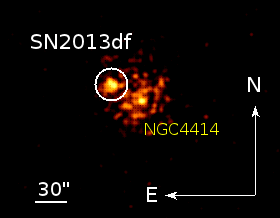
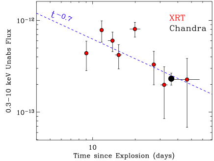
Figure 1.— Left panel: X-ray emission from SN 2013df is clearly detected by the Swift-XRT (0.3-10 keV). The image comprises observations collected starting June 13, 2013 until August 6, 2013, total of $49.5$ ks (i.e. $\sim 8-60$ days since explosion). Right panel: The X-ray emission from SN 2013df as captured by the Swift-XRT and Chandra X-ray Observatory (CXO) shows a temporal decay consistent with a power-law $t^{-\alpha}$ with best-fitting $\alpha=0.71\pm 0.16$ (1 $\sigma$ c.l.).

The X-Ray Telescope (XRT, Burrows et al. 2005) onboard the Swift satellite (Gehrels et al., 2004) started observing SN 2013df on 2013 June 13 ($\delta t=8$ days since explosion, PI Roming). We analyzed the XRT data using HEASOFT (v6.15) and corresponding calibration files. Standard filtering and screening criteria were applied. A fading X-ray source is clearly detected at the position of SN 2013df that we associate with the SN shock interaction with the medium (Fig. 1).

Figure 1 shows the temporal evolution of the X-ray emission from SN 2013df. We find a decay consistent with a power-law $\propto t^{-\alpha}$ with $\alpha=0.71\pm 0.16$ (1 $\sigma$ c.l.). The contribution of diffuse X-ray emission from the host galaxy to the Swift-XRT data has been estimated and subtracted by using the Chandra X-ray observations below (section 2.3.2) where the point-like emission from SN 2013df is well resolved.

A combined spectrum made from the entire Swift-XRT data set is well modeled by an absorbed power-law with hard photon index $\Gamma=1.58\pm 0.06$ ($1\sigma$) and no evidence for neutral hydrogen absorption intrinsic to the host galaxy, in agreement with the results from the spectral analysis of Chandra observations which we discuss in the next section 2.3.2. The Galactic neutral hydrogen column density in the direction of SN 2013df is $N_{H_{MW}}=1.60\times 10^{20}\,\rm{cm^{-2}}$ (Kalberla et al., 2005).

2.3.2 Chandra

We initiated deep X-ray follow up of SN 2013df with the Chandra X-ray Observatory on 2013 July 10, corresponding to $\delta t=36$ days since explosion (PI Soderberg). Data have been reduced with the CIAO software package (version 4.6) and corresponding calibration files. Standard ACIS data filtering has been applied. In this observation which lasted for 9.9 ks we clearly detected SN 2013df, with significance $>50\,\sigma$. As for the Swift-XRT observations, the spectrum is well modeled by an absorbed power-law with a hard photon index $\Gamma=1.26\pm 0.25$ ($1\sigma$). We again find no evidence for intrinsic neutral hydrogen absorption, with a $3\sigma$ upper limit of $N_{H_{int}}<2\times 10^{21}\,\rm{cm^{-2}}$. The complete X-ray light-curve of SN 2013df comprising Swift-XRT and Chandra observations is presented in Figure 1.

The hard X-ray spectrum can be fit by a thermal bremsstrahlung model with $kT>5$ keV (Figure 2). Due to relatively small number of counts and lack of coverage in hard X-ray band, we could establish only a lower limit on the plasma temperature.

3. Inverse Compton Model

The main radiation process powering radio SNe is synchrotron emission. A shock wave is an efficient way to convert bulk kinetic energy into thermal motion of the shock accelerated particles. The SN shock wave accelerates electrons to relativistic speeds which then gyrate in the shock amplified magnetic field and radiate synchrotron radiation. The electrons are usually assumed to have a power-law energy distribution, $n_{e}(\gamma_{e})\propto\gamma^{-p}_{e}$, with index $p$ and Lorentz factor $\gamma_{e}$ of individual electrons as a proxy of electron energy. This form of the electron distribution is evident from the synchrotron radio spectrum.

Two radiative cooling processes can affect this particle distribution: synchrotron cooling and inverse Compton scattering (IC). The synchrotron, as well as IC, power of an individual electron is strongly dependent on its Lorentz factor, $P_{\nu}\propto\gamma^{2}_{e}$. As a result, high energy electrons tend to cool down faster. The cooling timescale for electrons emitting synchrotron radiation at frequency $\nu$ is given by Björnsson & Fransson (2004) as

$$t_{sc}=1.7\times 10^{2}B^{-3/2}\nu^{-1/2}_{10}\rm days$$ (1)

when $\nu_{10}\equiv\nu/10^{10}$ Hz . Thus, the synchrotron cooling will be dominant only when $t_{syn}$ is the smallest timescale in the system i.e. $t_{sc}\ll(t,t_{ic})$.

The particle distribution could also be affected when high energy electrons cool down by scattering off optical photons due to photospheric emission from the SN. In the process, electrons cool down by imparting a fraction of their energy to the photons. The cooling time scale for this process depends on the reservoir of optical photons. For a SN having bolometric luminosity $L$ and size $r$ the average photon energy density would be given by $U_{ph}=L/4\pi r^{2}c$. Using this the cooling time scale is given by

$$t_{ic}=1.5\frac{B^{1/2}~{}r^{2}_{15}}{L_{42}~{}\nu^{1/2}_{10}}~{}\rm days$$ (2)

There is another way of demonstrating the importance of IC as the dominant cooling process over synchrotron emission. It can be shown that the cooled down electrons have a steeper Lorentz factor distribution $n_{e}(\gamma_{e})\propto\gamma^{-(p+1)}_{e}$ which is similar in the case of IC and synchrotron cooling, since both the processes have similar dependence on electron Lorentz factor: $P_{\nu}\propto\gamma^{2}_{e}(U_{B}+U_{ph})$. If the local magnetic field energy density ($U_{B}$) dominates over the local photon energy density ($U_{ph}$), synchrotron cooling will be stronger than IC cooling and vice-versa. The effective electron distribution, and therefore the resultant radiation spectrum, will display only one break but its evolution with time will be determined by the dominant cooling process responsible for the break.

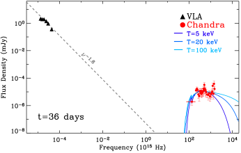
Figure 2.— Radio to X-ray SED of SN 2013df at the time of the Chandra observations. The X-ray flux is clearly in excess to the synchrotron model that best fits the radio observations (grey dashed line) and can be explained by thermal bremsstrahlung emission with temperature $T>5$ keV. Observations at $E>10$ keV such as might be done by NuSTAR is necessary to constrain the temperature of the emitting plasma.

Let $\gamma_{sc}$ and $\gamma_{ic}$ be the characteristic Lorentz factors where the distribution of emitting particles steepens due to the synchrotron and IC cooling, respectively:

$$\gamma_{sc} =8.9\times 10^{3}~{}B^{-2}~{}t^{-1}_{d}$$ (3)

$$\gamma_{ic} =134~{}r^{2}_{15}~{}L^{-1}_{42}~{}t^{-1}_{d}$$ (4)

The characteristic synchrotron frequency of emission due to an electron of Lorentz factor $\gamma_{e}$ is $\nu_{e}=1.2\times 10^{6}B\gamma^{2}_{e}$ Hz. Using this, the ratio of synchrotron and IC cooling break frequencies would be $(\nu_{sc}/\nu_{ic})\propto L^{2}_{42}\,B^{-4}\,r^{-4}_{15}$. We assume that the magnetic field energy density is a constant franction ($\epsilon_{B}$) of the thermal energy density behind the shock and $\epsilon_{B}\approx 0.1$. The thermal energy density behind the shock wave is given by $U=(9/8)nm_{p}\beta^{2}c^{2}$. Expressing the CSM density $n$ in terms of mass-loss rate ($\dot{M}$ in units of $10^{-6}\,\rm M_{\odot}/yr$ and wind velocity $v_{w}$ in units of $1000\,\rm km/s$) and $r=\beta\,ct$ for a freely expanding shock wave, gives the ratio of the break frequencies to be;

$$\left(\frac{\nu_{sc}}{\nu_{ic}}\right)=2.6\times 10^{3}\,\frac{L^{2}_{42}}{\beta^{4}_{-1}\,\epsilon^{2}_{B,-1}}\,\left(\frac{\dot{M}_{-6}}{v_{w,3}}\right)^{-2}$$ (5)

It is important to note that this ratio is independent of the source size. We can therefore state a general result that for low to intermediate mass-loss rates ($\dot{M}\leq 10^{-5}\,\rm M_{\odot}/yr$) the dominant cooling process in the radio SNe would be inverse Compton rather than synchrotron cooling.

The only time dependence in equation 5 is through the evolution of photospheric emission expressed as $L_{42}$. The optical peak brightness is typically reached around 20 days after the SN. Since $\nu_{sc}\propto t_{d}$, which follows from Equation 4 and subsequent discussion, it can be shown that the synchrotron cooling break is already out of the radio frequency bands by the time SN is at its peak bolometric luminosity. Therefore, the synchrotron cooling break would not be visible in typical radio SNe.

Having demonstrated that the early steep radio SED is likely due to the IC scattering of optical photons, we now proceed to discuss model fitting and estimation of physical parameters for SN 2013df.

4. Model Fits, Spectral and Physical Parameters

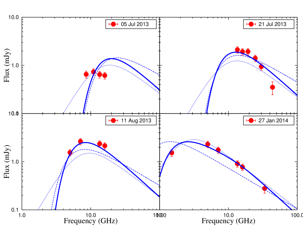
Figure 3.— Radio SED of SN 2013df at different epochs. The lines indicate the best fit models: SSA as the dotted lines, FFA $\otimes$ SSA as the dashed lines and IC $\otimes$ FFA $\otimes$ SSA as the solid lines.

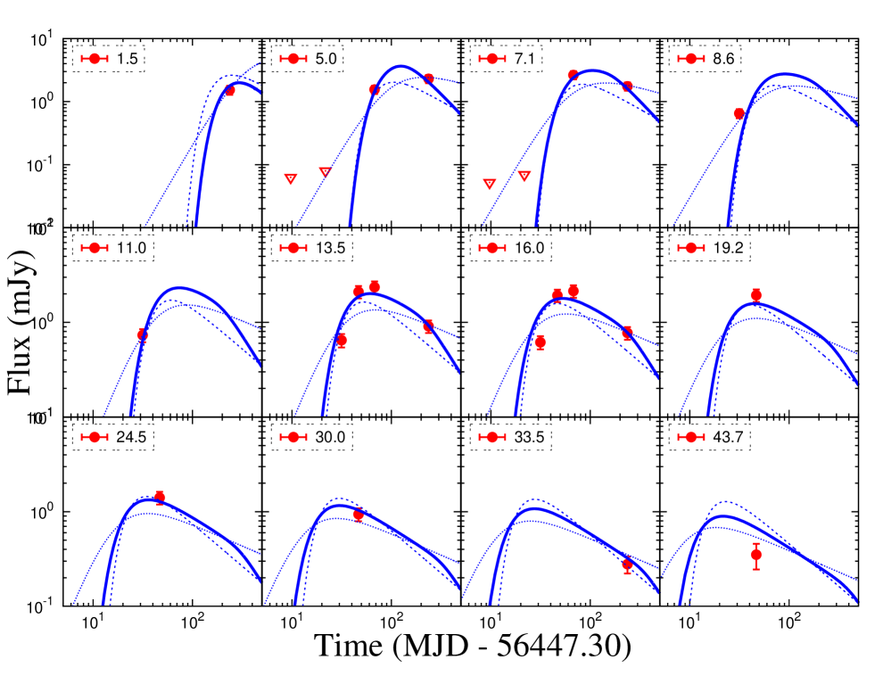
Figure 4.— Radio light curves of SN 2013df at various radio-frequency bands. The lines indicate the best fit models: SSA as the dotted lines, FFA $\otimes$ SSA as the dashed lines and IC $\otimes$ FFA $\otimes$ SSA as the solid lines.

As discussed in the previous section IC cooling modifies the electron distribution and consequently the synchrotron emission. Evolution of this electron distribution with time depends on the bolometric luminosity as well as the size of the SN. In order to parametrize this evolution we have characterized the SED using the synchrotron self-absorption break frequency ($\nu_{a}$), the characteristic synchrotron frequency due to electrons with the minimum Lorentz factor ($\nu_{m}$) and the inverse Compton cooling break frequency ($\nu_{ic})$, as well as the spectral peak $f_{\nu_{a}}$ of the synchrotron spectrum. In the appendix, we provide spectral and temporal scalings for the evolution of these spectral breaks.

To fit all the radio observations collectively we followed a procedure similar to that of Kamble et al. (2014) and scalings from the Appendix here. By using least square minimization we estimated values for the spectral peak $f_{\nu_{a}}$, break frequencies $\nu_{a},\nu_{ic}$, frequency of free-free absorption $\nu_{\rm ff}$ where optical depth to free-free absorption $\tau_{\rm ff}=1$ (for definition see Equation 6 below), electron distribution index $p$ and deceleration parameter $m$. The bolometric luminosity of SN 2013df was used as an input to determine the evolution of $\nu_{ic}$.

The statistical uncertainties in flux densities measured and listed in Table 1 are the respective image RMS. Variations in the local weather at the telescope can introduce additional errors to the measured image RMSs. Furthermore, calibration of the flux and phase calibrators can add further systematic errors of a few percentage. Therefore, during the model fitting, about $15\%$ of the total error was added in quadrature to account for these sources of errors.

The radio SED indicate that the frequency $\nu_{m}<\nu_{a}$ during all the observations and in any case is below the observing band. As a result, we can constrain the spectral break $\nu_{m}\ll 1$ GHz.

The best fit value of spectral peak flux density is determined to be $f_{\nu_{a}}=48\pm 5$ mJy at the self-absorption frequency $\nu_{a}=3.3\pm 0.5$ GHz on 21st July 2014 or at $t=46.8$ days after the burst and the best fit reduced $\chi^{2}=5.2$ per degrees of freedom (DOF) for 14 DOF. We note that a significant contribution to the $\chi^{2}$ comes from the earliest epoch of radio detections on 05 July 2013. Dropping those observations from the fit results in a significant improvement with reduced $\chi^{2}=1.7$ for 10 DOF. The resultant model SEDs are compared with observations in Figure 3 and the light-curves in Figure 4.

The Figures 3 and 4 highlight the importance of individual emission and suppression processes such as SSA (synchrotron self-absorption), FFA (free-free absorption) and IC (inverse Compton). At early epochs, the model synchrotron emission is under-estimated and can not anticipate the subsequent rise very well. The rising SEDs suggest an accelerating shock wave with $\alpha_{r}=1.12$ (see EquationA2). The best fit parameters obtained using the SSA model alone (reduced $\chi^{2}=3.8$ for 16 DOF), $f_{\nu_{a}}=1.8$ mJy and $\nu_{a}=15.6$ GHz result in an unrealistically slow shock wave $v_{sh}=0.02\,c$. This is significantly slower than the velocities estimated by the emission lines in optical spectra and typical ejecta velocities of $v_{ej}\approx 10,000$ km/s in SNe. This, therefore, clearly indicates that the free-free absorption must be playing an important role in SN 2013df.

Inclusion of free-free absorption improved the estimates of the shock velocity consistent with the typical values, but not necessarily the quality of the fits (reduced $\chi^{2}=6.8$ for 15 DOF). The SSA and SSA$\otimes$FFA models however result in shallower SEDs which do not agree well with observations at early epochs, most notably on 21st July 2013. The steep spectral shape should be related to the underlying steep electron energy distribution and therefore could be the result of a cooling process. As discussed in section $\S$ 3 inverse Compton cooling is likely to play the significant role. We therefore believe that the steep SED is the result of inverse Compton cooling process.

At late epochs, the radio emission at GHz frequencies is expected to be less affected by the suppression effects: a) the synchrotron self absorption ($\nu_{a}$) falls below GHz bands, b) effects of free-free absorption diminishes rapidly with increasing SN size as the optical depth to free-free absorption $\rm\tau_{ff}\propto r^{-3}$ and c) inverse Compton cooling becomes insignificant as the reservoir of optical photons is drained off with diminishing bolometric luminosity. As a result, all three model estimates roughly agree with each other on the last epoch of observations on 27th January 2014 i.e. about 237 days after the SN.

For the electron energy distribution index, the fit converged to $p=2.7\pm 0.3$. The observations before 50 days show significant effects of inverse Compton cooling through the steep spectral index $\nu^{-\beta}$ where $\beta=1.6\pm 0.2$. As discussed in the appendix this spectral regime is related to the electron distribution index through $\beta=p/2$ and is consistent with the measured $p=2.7\pm 0.3$. At later epochs, when the inverse Compton subsides, optically thin synchrotron spectrum is related to the electron distribution as $\beta=(p-1)/2$. The observed $\beta=0.9\pm 0.1$ is therefore consistent with it.

The shock wave expansion is best fit as $r=r_{0}(t/t_{0})^{\alpha_{r}}$ with $\alpha_{r}=0.84\pm 0.1$ (see Equation A2). This is consistent with the expectations for a compact, radiative envelope star where the outer density profile should tend to a power law in radius, $\rho_{sn}\propto r^{-10.2}$ giving $\alpha_{r}=0.88$ (Chevalier, 1982; Matzner & McKee, 1999). Our estimate $\alpha_{r}=0.84\pm 0.1$ is also consistent with a convective outer envelope ($\rho_{sn}\propto r^{-12}$) where one expects $\alpha_{r}=0.9$.

4.1. X-rays as Thermal Bremsstrahlung emission

X-ray emission in SNe could be produced by one of the three radiation processes: synchrotron, inverse Compton and bremsstrahlung. Using the radio spectral index of $\beta=-1.6$ based on observations and modeling of the radio emission, we expect the synchrotron emission in X-ray bands to be more than two orders of magnitude fainter as shown in Figure 2.

Inverse Compton scattering of the photospheric optical emission in to the X-ray bands by relativistic non-thermal electrons behind the forward shock is another possibility. The X-ray spectrum produced by such scattering would be soft. The spectral photon index of the observed X-ray emission in SN 2013df ($\Gamma=1.3$) is, however, significantly hard and is incompatible with a spectrum dominated by Comptonization. Instead, such a hard spectrum is consistent with the expectations from thermal bremsstrahlung emission.

SN 1993J was another type IIb supernova with bright X-ray emission detected for up to several tens of days. Fransson, Lundqvist, & Chevalier (1996) modeled it using the thermal bremsstrahlung emission from the forward and reverse shocks that propagate into the stellar wind and ejecta, respectively. Following a detailed analytic argument Fransson, Lundqvist, & Chevalier (1996) showed that the reverse shock was radiative and most of the X-ray emission during the first few months originated in the forward shock. They estimated the pre-SN mass-loss rate to be $\sim 4\times 10^{-5}~{}\rm M_{\odot}/yr$ for a wind velocity of 10 km/s.

Following the procedure outlined in Fransson, Lundqvist, & Chevalier (1996), we come to the similar conclusions for SN 2013df as those for SN 1993J. In Figure 5 we show a range of mass-loss rates and forward shock velocities to compare the resultant X-ray flux due to thermal bremsstrahlung emission with observations.

As pointed out by Fransson, Lundqvist, & Chevalier (1996) the X-ray emission may originate either in the forward shock that is sweeping the dense pre-SN wind or in the reverse shock that forms at the contact discontinuity and propagates into the denser ejecta. For homologous expansion, as is approximately the case for SNe, it is convenient to express the ejecta density profile is as a function of velocity, v, as $\rho_{sn}\propto v^{-n}$. The reverse shock temperature may depend on this density profile. Following Fransson, Lundqvist, & Chevalier (1996), we find that the temperature of the reverse shock $T_{rs}\geq 10^{7}$ K and that of the forward shock $T_{fs}\geq 10^{9}$ K for reasonable shock velocities $v_{sh}\geq 10^{4}$ km/s and density profile of the ejecta $n\leq 15$.

If the reverse shock is radiative then a cool shell forms between between the reverse and forward shocked material which absorbs all the X-rays from the reverse shock. For $T>2\times 10^{7}$ K, cooling is dominated by bremsstrahlung emission and below that it is dominated by line emission. At such temperatures reverse shock remains radiative for a significant amount of time. For $\dot{M}\geq 8\,\rm M_{\odot}/yr$, $n\geq 12$ and $v_{sh}\leq 21,000$ km/s we find that the reverse shock remains radiative for at least 50 days after the SN which spans the entire duration of our X-ray observations. Thus, all X-rays from the reverse shock are absorbed and most of the observed X-ray flux is due to the forward shocked material.

Chandra observation provides the best constraints on the model parameters. The red shaded area in Figure 5 corresponds to $3\sigma$ contour bounded by $(6.1\leq\dot{M}\leq 10.1)\times 10^{-5}\,M_{\odot}$/yr ($v_{w}=10$ km/s) with the forward shock velocity being ($0.05\leq\beta\leq 0.1$). The corresponding mass-loss rates for the $5\sigma$ contours shown in larger shaded area are ($4\leq\dot{M}\leq 11.1)\times 10^{-5}\,M_{\odot}$/yr, $v_{w}=10$ km/s for similar shock velocities. The solid red line corresponding to the best model estimate for reproducing Chandra observations gives $\dot{M}=8.3\times 10^{-5}\,M_{\odot}$/yr, $v_{w}=10$ km/s and $\beta=0.07$.

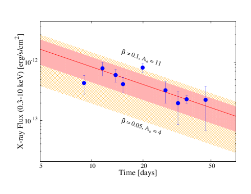
Figure 5.— Thermal bremsstrahlung emission in X-rays. The Chandra and Swift observation are shown as blue data points. The modelled thermal bremsstrahlung emission is shown by the shaded region. The lower bound corresponds to the shock velocity $\beta=0.05\,c$, mass-loss rate parameter $A_{*}=4$ and the upper bound to $\beta=0.1,A_{*}=11$.

4.2. Model Parameters from Radio Emission

Another effect of the stellar mass loss is in the form of absorption of radio emission by the ionized wind surrounding the SN. The free-free absorption optical depth of this unshocked gas at frequency $\nu$ is given by

$$\tau_{\rm ff}\approx 1.9~{}A^{2}_{*}\left(\frac{\rm T}{5\times 10^{4}\,\rm K}\right)^{-3/2}\left(\frac{\nu}{\rm GHz}\right)^{-2}\left(\frac{\beta}{0.1}\right)^{-3}\left(\frac{\rm t}{25\,\rm day}\right)^{-3}$$ (6)

where $\beta$ is the shock velocity in units of the speed of light and and A* is the mass loss rate in terms of a reference value of $5\times 10^{13}$ gm/cm. The mass loss parameter $A=\dot{M}/4\pi V_{w}\rm gm~{}cm^{-1}$ and our reference value of $5\times 10^{13}$ gm/cm is attained for $\dot{M}=10^{-5}M_{\odot}/\rm yr$ and $v_{w}=10$ km/s.

At $\rm t=46.8\,day$ after the SN, our best fit model gives $\tau_{\rm ff}=1$ at $\nu=10\pm 1$ GHz. Equation 6 can then be used to get the mass loss rate parameter in terms of shock velocity $\beta$ as $A_{*}=584\,\beta^{3/2}$.

Following Kamble et al. (2014), we express the synchrotron frequency and flux in terms of unknown model parameters:

$$\nu_{a} = 4.0\times 10^{11}A_{*}^{0.65}\left(\frac{\beta}{0.1}\right)^{0.72}\left(\frac{\epsilon_{B}}{0.1}\right)^{0.35}\left(\frac{\epsilon_{e}}{0.1}\right)^{0.51}\left(\frac{\rm t}{\rm day}\right)^{-1}\rm GHz$$ (7)

$$f_{\nu_{a}} = 0.35A_{*}^{1.37}\left(\frac{\beta}{0.1}\right)^{3.79}\left(\frac{\epsilon_{B}}{0.1}\right)^{0.63}\left(\frac{\epsilon_{e}}{0.1}\right)^{1.27}\left(\frac{d_{L}}{100\rm\,Mpc}\right)^{-2}\rm mJy$$ (8)

where $\epsilon_{e}$ and $\epsilon_{B}$ are the fractions of thermal energy behind the shock that goes into accelerating electrons and magnetic fields, respectively.

Using the best fit spectral parameters determined from radio emission modeling described in the previous section one can simultaneously solve Equations 8 and 6 for physical parameters $\beta,\epsilon_{e}$ and $\epsilon_{B}$. Using this approach we estimate the shock velocity to be $\beta=0.07\pm 0.01$ which is faster that the velocity of the fastest ejecta estimated from the optical line-widths of about $10,000$ km/s (Morales-Garoffolo et al., 2014; Ben-Ami et al., 2014; Van Dyk et al., 2014; Maeda et al., 2015). This estimate is also consistent with the thermal bremsstrahlung emission observed in X-rays (see Figure 1). For SN 1993J the velocity estimated from optical lines was about $19,000$ km/s, and a shock velocity was estimated to be $21,600-24,700$ km/s (Fransson & Björnsson, 1998) in agreement with the VLBI measurements of Bartel et al. (1994, 2002), which gives $\beta=0.073$, same as that estimated above for SN 2013df. The SN mass-loss rate is then estimated to be $\dot{M}=10.5\pm 3.0\,\rm M_{\odot}/yr$ for the wind velocity of $v_{w}=10\,\rm km/s$, in agreement with the estimates from the X-rays. It is reassuring that in an independent approach Maeda et al. (2015) reach roughly similar conclusions using late time optical evolution of SN 2013df.

Similarly, we determine $\epsilon_{e}=0.2\pm 0.02$ and $\epsilon_{B}=(1.0\pm 0.1)\times 10^{-3}$. While this determined value of $\epsilon_{e}$ is similar to those generally found in SNe, we find a significant deviation from energy equipartition between magnetic fields and accelerated particles. For comparison, Fransson & Björnsson (1998) deduced $\epsilon_{B}=0.14$ for SN 1993J. The high mass-loss rate combined with low $\epsilon_{B}$ may be the reasons for unusual radio properties of SN 2013df. The only other SN for which inverse Compton effect was shown to be of importance in shaping radio and X-ray emission was SN 2002ap, a type Ic supernova. It is interesting to note that a low value of $\epsilon_{B}=2\times 10^{-3}$, similar to the present case of SN 2013df, was deduced for SN 2002ap also (Björnsson & Fransson, 2004).

4.3. Inverse Compton Cooling Break in Radio

The break in the energy distribution of relativistic electrons due to the IC cooling corresponds to a spectral break $\nu_{IC}$ discussed in section 3. Following that discussion, it can be shown in terms of the physical parameters

$$\nu_{IC}=1.4\times 10^{10}\frac{\beta^{4}_{-1}}{L^{2}_{42}}\left(\frac{\dot{M}_{-5}}{v_{w,1}}\right)^{-2}t_{d}\sqrt{\epsilon_{B,-1}}\,{\rm Hz}$$ (9)

Due to its strong dependence on shock velocity, $\nu_{IC}$ favors a slow shock wave and lower mass-loss rates. We obtained $\nu_{IC}=0.6\,\rm GHz$ at $t_{0}=46.8$ days for the best fit to the observations. The bolometric luminosity of SN 2013df at that epoch is $\approx(0.8\pm 0.3)\times 10^{42}$ erg/s (Morales-Garoffolo et al., 2014). For these observables one can estimate a combination $\beta\epsilon^{2/19}_{B}=0.01$. For the fastest line velocities $\beta=0.04$ which gives $\epsilon_{B}=10^{-5}$. However, due to the strong dependence of $\nu_{IC}$ on other quantities, especially $L_{bol}$ and $\beta$, this comes with a large uncertainty $\epsilon_{B}=(1\pm 2)\times 10^{-5}$.

4.4. Inverse Compton emission in X-rays

The relativistic electrons which generate the synchrotron radiation and powers the radio emission in SN shock wave, will naturally up-scatter the optical photons that emerge from the photosphere of the SN. If the seed photons or the relativistic electrons have a wide energy distribution, the spectrum of the up scattered inverse Compton emission will also be wide. One can, however, estimate the total contribution of IC component in a quasi-monochromatic X-ray band. The resultant X-ray emission will be related to the energy distribution of electrons. The non-thermal electron distribution will produce non-thermal X-rays. In the process of IC scattering, the electrons lose their energy. Higher the electron Lorentz factor, faster it loses energy to inverse Compton. This, in turn, changes the shape of the electron distribution at higher Lorentz factor, making it steeper than the electron distribution injected at the shock front.

Radio observations of SNe are an excellent probe of the underlying electron distribution and magnetic field behind the shock. One can construct bolometric lightcurve of SNe using optical observations. Thus, between radio and optical, one has all the necessary information required to understand and estimate the inverse Compton emission. Below we use these observations to self-consistently model the IC emission.

From the previous section, radio observations on 21st July 2013, or at supernova age of $t_{0}=46.8$ days, indicate $B\approx 0.8$ G. Therefore, the magnetic field energy density behind the shock is $U_{B}=0.02\,\rm erg/cm^{3}$. Radio observations also indicate the size of the shock wave to be $r=10^{16}\,\rm cm$. From the optical observations we estimate the bolometric luminosity of the SN to be $L_{bol}\approx 0.8\times 10^{42}$ erg/s on the the same epoch. Thus, energy density in seed photons turns out to be $U_{ph}\approx 0.03\,\rm erg/cm^{3}$. Furthermore, $\xi(p=2.7)=3.06$ (see Equation B1 in the appendix), and $f_{\nu_{a}}=48$ mJy at the self-absorption frequency $\nu_{a}=3.3$ GHz. Using these values in Equation B1 and $p=2.7$ as determined from radio observations, we determine $F_{\nu}(1\,\rm keV)=2.3\times 10^{-6}$ mJy. This is more than an order of magnitude fainter than the observed X-ray emission.

Similarly, using Equation B1 and $p=2.7$, one can estimate the time evolution of IC X-ray flux to be $F_{\nu}(1\,\rm keV)\propto L_{bol}(t)^{0.963}\times t^{-0.925}$. The expected light curve of the IC X-ray emission in 1-10 keV band is significantly fainter. Overall, the contribution of the inverse Compton emission to observed X-ray emission is negligible.

In other words, the observed X-ray emission is too bright at all epochs than what is expected from the inverse Compton emission. One can therefore conclude that the X-rays from SN 2013df must be due to another strong emission component. X-ray brightness estimates due to thermal bremsstrahlung, as shown in the previous sections, appear to be reasonable.

5. Discussion

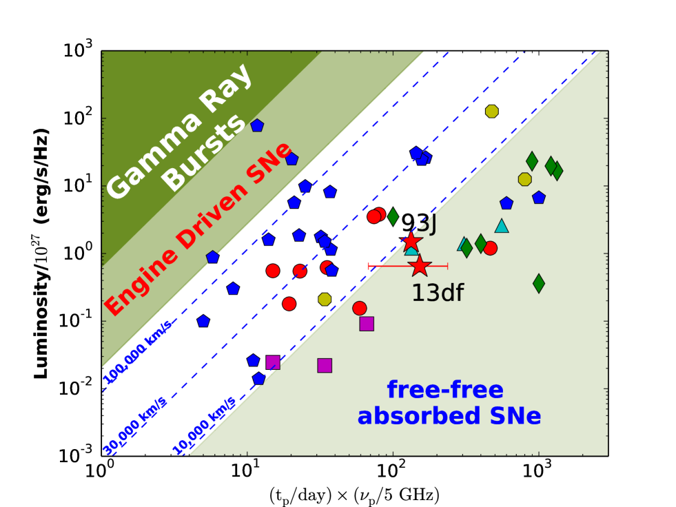
Figure 6.— Peak spectral radio luminosity v/s product of the peak time and frequency for radio SNe of various types - Ib/c: blue pentagons; IIb: red circles; IIP: magenta squares; IIn: green diamonds; IIL: cyan triangles and II (SN 1978K, 1981K & 1982aa): yellow octagons. The similarity between SN 1993J and SN 2013df is clearly evident in this plot.

5.1. Radio SNe - a global view

It is instructive to view the SN 2013df in comparison with radio SNe in general. The peak Luminosity v/s peak time plot offers the most informative way to project the radio SNe. The positions of radio SNe in such a plot are shown in Figure 6, which is an update of the previous plots in Chevalier (1998); Chevalier, Fransson, & Nymark (2006). Different SN types have been color coded for the ease of distinction - Ib/c: blue pentagons; IIb: red circles; IIP: magenta squares; IIn: green diamonds; IIL: cyan triangles and II (SN 1978K, 1981K & 1982aa): yellow octagons.

While both the co-ordinates of SNe on this plot are purely observables, the underlying lines depend, though weakly, on certain model assumptions. The blue dotted lines of constant shock velocity assume energy equipartition between synchrotron emitting electrons and magnetic field, and that there is no strong cooling of the electrons. The lines also assume a uniform electron energy distribution index of $p=3$. Despite these assumptions the plot provides an easy way of comparison between different SNe as well as insights into different classes of SNe and their progenitors.

The slowest to fastest moving objects appear from right to the left of the plot. The blue dotted lines indicate mean velocities of the radio shocks if SSA is the responsible for the spectral peak. The relativistic synchrotron sources such as gamma ray bursts appear to the far left of the plot in the dark green shaded area. The relativistic SNe, such as SN 2009bb, appear in the light green shaded area labelled as the engine driven SNe. As one moves to the right of the plot synchrotron emission is increasingly suppressed by the FFA in the progenitor wind.

The effect of FFA is often noticeable in radio observations where the SED falls faster than in the SSA towards low radio frequencies. Consequently, the rise of radio light curve is also faster at early times in the presence of FFA. Our early non-detections of SN 2013df at C band clearly bring out the presence of FFA. Ignoring FFA results in the estimates of reduced shock-velocity, which often fall short of photospheric velocities measured from optical line emission. Therefore, we use nominal a velocity of $<10,000$ km/s as a distinction between FFA and SSA region in the luminosity plot (Figure 6).

5.2. Progenitors of SNe IIb - extended versus compact

Figure 6 captures the essence of radio emission in SNe and portrays the diversity among various types of SNe. Radio SNe show a wide luminosity distribution spread over more than four orders of magnitude. Luminosity distribution of IIb SNe is significantly narrow, confined within two orders of magnitude. But their distribution of peak times is relatively as wide as those of SNe Ibc. The distribution merges with those of SN Ib/c. As one moves to the right, the effect of FFA becomes increasingly noticeable in SNe IIb as has been clearly seen in SN 1993J (Fransson & Björnsson, 1998), 2013df (this work), 2011hs (Bufano et al., 2014) and 2010P (Romero-Cañizales et al., 2014).

It is, therefore, plausible that the broad distribution in rise times of SN IIb may be an outcome of different intrinsic properties of the progenitors or the circumstances surrounding the SN. Indeed, such a proposal has been put forward by Chevalier & Soderberg (2010) based on distinct emission properties observed in radio, optical and X-rays.

One clue to this might come from early rapidly evolving optical emission often termed as the ‘cooling envelope emission’. Current understanding of this emission is that following the shock break-out from stellar surface, outer envelope of the star expands and cools. As the expanding photosphere reaches this stellar envelope the radiation stored in the envelope manages to escape. This ‘hot’ radiation results in the rapidly evolving UV/optical emission at early times lasting from a few hours to several days. The cases where such emission has been detected are only a few consisting of SNe of type IIb: 1993J, 2011dh, 2011hs, 2011fu and most recently 2013df, and type Ic: SN 2006aj and a few cases of SN of type IIP.

This however is not a complete picture. Observations are maturing rapidly in discovering SNe early, in carrying out rapid follow up and in UV capabilities. Rapid follow up reveals that SNe does not always develop such double peaked early optical emission. Despite observations at very early times, several SNe have been detected which do not show early optical emission to very deep limits which might be problematic to the theories of cooling envelope emission, especially if the SNe are expected to have similar progenitors. It may, therefore, be insightful to tie up such properties with multiband long term follow up observations.

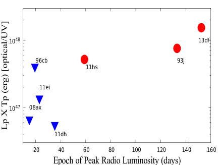
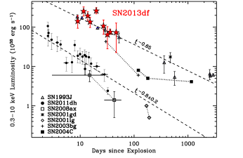
Figure 7.— Early optical emission and radio properties: A product of the early peak bolometric luminosity and its epoch are plotted against the epoch of radio peak brightness (Left panel). The quantity on the y-axis is a measure of the amount of energy a SN deposits in the envelope. The red points are the SNe with detected early optical emission. The blue upper limits are the SNe where early UV/optical observations have been reported without similar long lasting optical emission. The detections and non-detections of early optical peak are clearly separated signaling apparent dichotomy. X-ray emission in type IIb: Compared to a sample of type IIb SNe, SN 2013df shows luminous X-ray emission with strong similarities to SN 1993J, both in terms of luminosity and temporal decay rate (Right panel). The SNe with bright X-ray emission are also the ones which show FFA and delayed peak brightness in radio. References: SN 1993J (Chandra et al., 2009), SN 2001gd (Pérez-Torres et al., 2005), SN 2003bg (Soderberg, Chevalier, Kulkarni, & Frail, 2006), SN 2004C (Dittman in prep.), SN 2008ax (Roming et al., 2009), SN 2011dh (Soderberg et al., 2012).

A simple but surprising trend seem to emerge between this early optical emission and slowly evolving SNe. And at the moment we concern ourselves with of those of type IIb only. All SNe in the FFA region of Figure 6 exhibit this early optical emission whereas others do not ! As mentioned before, SNe 1993J, 2011hs, 2013df are the prime examples of this optical emission, they all show strong FFA absorption in the radio emission and reach radio peak brightness comparatively late ($\geq$ 100 days). SNe 2010P which also falls in the same FFA category was never observed in UV/optical so we can not comment on that. Opposite of this is SN 2011fu, which exhibited the early optical peak but was never followed up in radio so it is not possible to comment if it also had a strong FFA component. On the other hand, SNe without strong FFA do not show this optical emission to deep limits despite early observations (SNe 1996cb, 2008ax and 2011ei). Early UV/optical observations have not been reported for SN 2001gd and 2001ig. SN 2011dh is an interesting intermediate case, where the early optical emission was detected in one band and was significantly short lived. Also, its contribution to the bolometric luminosity is negligible. The progenitor of this SN has however been identified and we discuss that issue later.

These findings are put in persecutive and more quantitatively in Figure 7 where we plot the product of the early peak bolometric luminosity and its epoch against the epoch of radio peak brightness. The right panel of Figure 7 shows X-ray emission in SNe IIb. Interestingly, the bright X-ray emission correlates with radio properties such as FFA, delayed radio peak, and double peaked optical emission. Rapidly evolving radio SNe are also the ones which display faint or none X-ray emission. Unlike SN 1993J and 2013df, X-ray emission of SN 2011dh was non-thermal in nature and more than an order of magnitude fainter.

Early UV/Optical observations of SNe provide interesting diagnostics about the SN progenitor, especially in cases where pre-SN images of the progenitor do not exist. But before that the physical theories need to be cross checked and calibrated against the cases where the progenitor has been identified. Undoubtedly, such detections will improve in future and we will have more candidates to test theories against. At the moment we have four SNe with identified progenitors, properties of which we discuss in the next section.

5.3. SNe IIb with identified progenitors

Observations are not only getting quick in responding to the SNe fast enough to catch the early emission but also probing deeper to match and identify the progenitors from archival images of nearby SNe. As a result progenitors of four SNe of type IIb have been identified in pre-SN images. A YSG of radius $\approx 600\,R_{\odot}$ was identified as the progenitor of SN 1993J. A similarly large YSG star has been identified as a progenitor of SN 2013df. A less extended, a YSG nevertheless, with $R\approx 200R_{\odot}$ was found to have disappeared from the position of SN 2011dh and has therefore been concluded as the progenitor of SN 2011dh. With the surge in direct identification of SN progenitors it is now becoming increasingly possible to test some of the predictions about early emission properties of similar SNe.

The question then is why should similar kind of progenitors have different emission properties such as in the cooling envelope which emerge from close to the stellar surface ? As pointed out before not every type IIb SN shows cooling envelope emission, and there appears to be correlation with the progenitor size. Indeed, SN 2008ax did not display the cooling envelope emission. It was difficult to fit either a single or binary supergiant or WR + supergiant system self-consistently as progenitors to the observed colors from the pre-SN images (Li et al. 2008; Crockett et al. 2008). The possible initial mass range for the progenitor turns out to be large, $\approx 10-28\,M_{\odot}$.

More progress is required on theoretical front in figuring out all the elements for the CEE theory to be successful. It has been pointed out by Nakar & Piro (2014) that standard stellar density profile does not lead to CE emission. Instead, extended progenitors with non-standard density profiles are necessary. Such modifications of density profiles in the extended envelopes may occur only in a subset of progenitors due to binary interaction, non-standard mass-loss, episodic ejections of outer envelopes and subsequent evolution etc. There are, however, no direct means of observationally confirming if such modified density profiles actually exist elsewhere and more so under a given situation. Secondly, current theories do not take into account detailed dynamics or radiation transport as pointed out by Rabinak & Waxman (2011); Nakar & Sari (2010); Nakar & Piro (2014). Different kinds of progenitors, such as WR, BSG and RSG, have been considered by Nakar & Sari (2010); Nakar & Piro (2014) to estimate CE emission properties. One difference that is expected, and to which calculations from different groups agree, is that larger progenitor results in longer lasting CE emission.

A credible theory must explain all the apparent contradictions and complexities as pointed out above. This raises an important question: is the double peaked optical light curve really due to the CE emission ? Alternative ideas should be explored in order to explain observations satisfactorily. Interaction of shock-wave with binary companion is expected to leave some signature on the optical light curves. Such an idea has been explored for SN Ia where a white-dwarf accretes matter from the companion ultimately leading to the SN. As the SN shock-wave interacts with the envelope of the companion dissipating kinetic energy and heating it up, it results in the emission that is expected to peak in UV bands on timescales of a few days which is roughly similar to that observed in some type IIb. It is of considerable interest that a binary companion has also been either confirmed (SN 1993J, SN 2011dh) or speculated to the progenitors of these SNe.

SNe of type IIb thus provide the best opportunities to study variety of phenomena: double peaked bolometric light curves and bright radio and X-ray emission. Due to the relatively higher rate of type IIb compared to Ibc they are also best suited for direct detection of progenitors. With the possibility of such rich datasets they are ideal for tying together various observed properties and in building a detailed understanding. Correlating progenitors with radio properties may be more subtle than the simple dichotomy of compact and extended progenitors and may be made more complex by the processes that affect stellar evolution such as stellar rotation, magnetic fields, binary interactions and evolution in the late stages (Smith & Tombleson, 2015). A more complete picture can be built by multiband observations and direct detection of progenitors in the pre-SN images.

6. Summary and Conclusions

We presented extensive radio and X-ray observations of SN 2013df in the context of type IIb SN explosions. We also presented a model of inverse Compton cooling and estimated its effects on the evolution of radio emission from SN 2013df. Our main results can be summarized as follows:

• With bolometric luminosities within a factor of a few of each other, and similarly extended luminous cooling envelope emission and comparable mass-loss rate estimates from the radio and X-ray emissions, SN 2013df appears similar to that of SN 1993J, in several ways. This close association is portrayed most easily in Figure 6. Indeed, the progenitor of SN 2013df appears to have been similar to that of SN 1993J in mass and radius (Van Dyk et al., 2014).

• SN 2013df showed a peculiar soft-to-hard temporal evolution of the optically thin part of the radio spectrum. We interpret this behavior as free-free absorbed synchrotron radiation where the underlying electron distribution responsible for the radio emission is modified by Inverse Compton cooling at early times (ref to Fig. 3). This model provides a reasonably good match to the observations for $t>40$ days and leads to the picture of a shock wave propagating with modest velocity $v_{sh}=0.07c$ into a dense environment, previously shaped by substantial mass loss from the progenitor star $\dot{M}=8\times 10^{-5}\,\rm{M_{\odot}/yr}$ (for wind velocity $v_{w}=10\,\rm{km\,s^{-1}}$). Comparable mass-loss rate was inferred for the type IIb SN 1993J (Fransson, Lundqvist, & Chevalier, 1996).

• Self-consistent modeling of the radio emission of SN 2013df that includes synchrotron emission and self absorption, free-free absorption and inverse Compton cooling effects shows significant deviation from the generally assumed equipartition of shock energy between magnetic fields and accelerated electrons. For SN 2013df we infer $\epsilon_{e}\sim 200\epsilon_{B}$.

• In close similarity to SN 1993J, the X-ray emission from SN 2013df (Fig. 7) is in clear excess with respect to the synchrotron model that best fits the radio emission (ref Fig. 2). The hard X-ray spectrum is dominated by thermal bremsstrahlung emission with $T>5$ keV and indicates a mass-loss rate $(4<\dot{M}<11)\times 10^{-5}\,\rm{M_{\odot}/yr}$, consistent with our results above.

• Our modeling of the radio and X-ray radiation from SN 2013df further demonstrates the importance of the IC cooling process in shaping the electron distribution responsible for the detected radio emission in SNe at early times.

• Finally, we observationally link the presence of bright cooling envelope emission in the optical/UV bands at very early times in type IIb SNe to the later appearance of heavily free-free absorbed radio emission (Fig. 7), coupled with hard X-ray radiation from thermal bremsstrahlung (and hence large mass-loss rate of the progenitor star before exploding). The dichotomy of such emission properties displayed by type IIb SNe suggest diversity among progenitors.

• The current small number of type IIb SNe well observed in the optical/UV, radio and X-ray bands both at early and at late times (Fig. 7) does not allow us to quantitatively test our conjectures. Clearly, a significantly larger sample of type IIb SN explosions with extended multi-wavelength coverage is needed. The case of SN 2013df demonstrate that multi-band observations provide crucial diagnostics about the nature of SN progenitors. SNe of type IIb are advantageous to carry out multi-faceted investigations including detections of progenitors in pre-SN observations, double peaked optical emission and non-thermal emission.

Appendix A Synchrotron Emission from Inverse Compton Cooled Electrons in Young Supernovae

Synchrotron spectrum produced by the relativistic electrons behind a non-relativistic shockwave expanding into the surround medium of density profile $n(r)\propto r^{-2}$ could be described as a broken power law with two characteristic frequencies ($\nu_{m},\nu_{a}$) and the spectral peak $F_{m}$. Following Soderberg, Chevalier, Kulkarni, & Frail (2006) and Kamble et al. (2014) we express the size and speed of the shockwave evolving in time as

$$r = r_{0}\times(t/t_{0})^{\alpha_{r}}$$ (A1)

$$\beta = \beta_{0}\times(t/t_{0})^{\alpha_{r}-1}$$ (A2)

where the shock speed is $\beta c=dr/dt$.

A.1. Spectral shape, Break Frequencies and Radio Light curves

We identify the spectral break due to inverse Compton cooling of electrons as a characteristic frequency ($\nu_{ic}$). The evolution of this break frequency depends not only on the SN size but also on its bolometric luminosity, $L_{bol}\propto t^{\alpha_{L}}$. Below we describe two spectral regimes that are most relevant for the evolution of radio SNe.

A.1.1 Case 1: $\nu_{m}\ll\nu_{a}\ll\nu_{ic}$

In Case 1, the characteristic synchrotron frequency is below the self-absorption frequency, $\nu_{m}\ll\nu_{a}$ and therefore the synchrotron emission is suppressed due to the self-absorption. As a result, the spectral peak occurs at $\nu_{p}\approx\nu_{a}$ and the scalings simplify to

$$\nu_{p}\approx\nu_{a}\propto t^{-\frac{(5p-2)-2\alpha_{r}(2p-3)}{p+4}},~{}~{}~{}f_{\nu_{p}}\approx f_{\nu_{a}}\propto t^{-(1-\alpha_{r})\frac{12p-7}{p+4}},~{}~{}~{}\nu_{ic}\propto t^{4\alpha_{r}-\alpha_{L}-3},~{}~{}~{}$$ (A3)

The temporal and frequency dependence of flux $f_{\nu}$ at observed frequency $\nu$ is then generalized by

$$f_{\nu}\propto\begin{cases}\nu^{5/2}~{}t^{2\alpha_{r}+1/2}&\nu_{m}<\nu<\nu_{a}\\ \nu^{-(p-1)/2}~{}t^{-[(5p-3)/2-\alpha_{r}(2p-1)]}&\nu_{a}<\nu<\nu_{ic}\\ \nu^{-p/2}~{}t^{-[5p/2-\alpha_{r}(2p+1)+\alpha_{L}]}&\nu_{ic}<\nu\end{cases}$$ (A4)

A.1.2 Case 2: $\nu_{m}\ll\nu_{ic}\ll\nu_{a}$

In Case 2, the synchrotron self-absorption frequency is above the characteristic inverse Compton frequency, $\nu_{ic}\ll\nu_{a}$. Since inverse Compton effect dominates around the epoch of peak bolometric brightness this situation is likely to occur around the peak optical brightness of the SN. The synchrotron spectral peak would still be at $\nu_{a}$ and the scalings are given by

$$\nu_{p}\approx\nu_{a}\propto t^{-\frac{5p-1}{p+5}(1-\alpha_{r})-\alpha_{r}},~{}~{}~{}f_{\nu_{p}}\approx f_{\nu_{a}}\propto t^{\frac{14p+5}{p+5}\alpha_{r}-\frac{13p}{p+5}+\alpha_{L}},~{}~{}~{}\nu_{ic}\propto t^{4\alpha_{r}-\alpha_{L}-3},~{}~{}~{}$$ (A5)

The temporal and frequency dependence of flux $f_{\nu}$ at observed frequency $\nu$ is then generalized by

$$f_{\nu}\propto\begin{cases}\nu^{5/2}~{}t^{4\alpha_{r}-\alpha_{L}-1/2}&\nu_{m}<\nu<\nu_{ic}\\ \nu^{5/2}~{}t^{4\alpha_{r}-\alpha_{L}-1/2}&\nu_{ic}<\nu<\nu_{a}\\ \nu^{-p/2}~{}t^{-[5p/2-\alpha_{r}(2p+1)+\alpha_{L}]}&\nu_{a}<\nu\end{cases}$$ (A6)

Appendix B Inverse Compton Scattering of photospheric emission

The same relativistic electrons which emit synchrotron emission are also responsible for the up-scattering of photospheric emission dominated by IR/optical/UV photons. If the scattering electrons have the power law energy distribution ($N(\gamma_{e})\propto\gamma^{-p}_{e}$), the up-scattered IC radiation carries the similar form ($E^{-(p-1)/2}$). The situation under consideration, IC scattering of Planck distributed photons by relativistic power-law electrons, has been considered in detail by Rybicki & Lightman 1979. Following equation 7.31 and 6.36 of Rybicki & Lightman (1979) we get a simple relation

$$\frac{P_{\nu,syn}}{P_{\nu,X}}=\left(\frac{\nu_{Syn}}{\nu_{X}}\right)^{-\frac{p-1}{2}}\frac{U^{\frac{p+1}{4}}_{B}}{U^{\frac{p+5}{8}}_{ph}}\times\xi(p)$$ (B1)

where we have collected the natural constants $h,c,q,m_{e}$ and dependence on parameter $p$ inside the function $\xi(p)$. We have plotted this function in Figure 8. The frequency $\nu_{X}$ is the frequency of the up-scattered photons. We use the subscript X to distinguish it from the inverse Compton cooling break $\nu_{ic}$ discussed in the previous section.

For $p=3.0$, Equation B1 reduces to the well known result

$$\frac{\nu_{syn}\times P_{\nu,syn}}{\nu_{X}\times P_{\nu,X}}\approx\frac{U_{B}}{U_{ph}}$$ (B2)

where factor $\xi(p)$ is often neglected.

The essence of Equation B1 is that the knowledge of electron distribution and seed photon field, from radio and optical observations respectively, is sufficient to describe the inverse Compton emission completely. For example, it follows from Equation B1 that for $p=3.0$ the IC flux is

$$F_{\nu,X}=\frac{1}{0.24}\,F_{\nu,syn}\left(\frac{\nu_{X}}{\nu_{syn}}\right)^{-1}\frac{U_{ph}}{U_{B}}$$ (B3)

where $U_{B}=B^{2}/8\pi$ and $U_{ph}=L_{bol}(t)/4\pi r^{2}c$. The ratio of energy densities $U_{ph}/U_{B}\propto L(t)$ in the simple case of freely expanding shockwave ($\alpha_{r}=1$), since $B\propto 1/r$ in the wind medium. Optically thin synchrotron flux in a given band $F_{\nu,syn}\propto t^{-1}$. This gives the scaling of inverse Compton flux as

$$F_{\nu,X}\propto L(t)\times t^{-1}$$ (B4)

similar to that given by Björnsson & Fransson (2004); Chevalier, Fransson, & Nymark (2006). From Equation B1 we can now show that for other values of p,

$$F_{\nu,X}\propto L(t)^{\frac{p+5}{8}}\times t^{-\frac{p+1}{4}}$$ (B5)

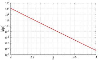
Figure 8.— The function $\xi(p)$.

References

- Aldering, Humphreys, & Richmond (1994) Aldering, G., Humphreys, R. M., & Richmond, M. 1994, AJ, 107, 662
- Baron et al. (1993) Baron, E., Hauschildt, P. H., Branch, D., Wagner, R. M., Austin, S. J., Filippenko, A. V., & Matheson, T. 1993, ApJ, 416, L21
- Bartel et al. (2002) Bartel, N., et al. 2002, ApJ, 581, 404
- Bartel et al. (1994) Bartel, N., et al. 1994, Nature, 368, 610
- Ben-Ami et al. (2014) Ben-Ami, S., et al. 2014, arXiv:1412.4767
- Björnsson & Fransson (2004) Björnsson, C.-I., & Fransson, C. 2004, ApJ, 605, 823
- Bufano et al. (2014) Bufano, F., et al. 2014, MNRAS, 439, 1807
- Burrows et al. (2005) Burrows, D. N., et al. 2005, Space Sci. Rev., 120, 165
- Chandra et al. (2009) Chandra, P., Dwarkadas, V. V., Ray, A., Immler, S., & Pooley, D. 2009, ApJ, 699, 388
- Chevalier (1982) Chevalier, R. A. 1982, ApJ, 259, 302
- Chevalier & Fransson (2003) Chevalier, R. A., & Fransson, C. 2003, Supernovae and Gamma-Ray Bursters, 598, 171
- Chevalier (1998) Chevalier, R. A. 1998, ApJ, 499, 810
- Chevalier & Fransson (2006) Chevalier, R. A., & Fransson, C. 2006, ApJ, 651, 381
- Chevalier, Fransson, & Nymark (2006) Chevalier, R. A., Fransson, C., & Nymark, T. K. 2006, ApJ, 641, 1029
- Chevalier & Soderberg (2010) Chevalier, R. A., & Soderberg, A. M. 2010, ApJ, 711, L40
- Ciabattari et al. (2013) Ciabattari, F., et al. 2013, Central Bureau Electronic Telegrams, 3557, 1
- Cohen, Darling, & Porter (1995) Cohen, J. G., Darling, J., & Porter, A. 1995, AJ, 110, 308
- Crockett et al. (2008) Crockett, R. M., et al. 2008, MNRAS, 391, L5
- de Witt et al. (2015) de Witt, A., Bietenholz, M. F., Kamble, A., Soderberg, A. M., Brunthaler, A., Zauderer, B., Bartel, N., & Rupen, M. P. 2015, arXiv:1503.00837
- Drout et al. (2013) Drout, M. R., et al. 2013, ApJ, 774, 58
- Ensman & Woosley (1987) Ensman, L., & Woosley, S. E. 1987, BAAS, 19, 757
- Filippenko (1997) Filippenko, A. V. 1997, ARA&A, 35, 309
- Filippenko (1988) Filippenko, A. V. 1988, AJ, 96, 1941
- Filippenko, Matheson, & Ho (1993) Filippenko, A. V., Matheson, T., & Ho, L. C. 1993, ApJ, 415, L103
- Fox et al. (2014) Fox, O. D., et al. 2014, ApJ, 790, 17
- Fransson & Björnsson (1998) Fransson, C., & Björnsson, C.-I. 1998, ApJ, 509, 861
- Fransson, Lundqvist, & Chevalier (1996) Fransson, C., Lundqvist, P., & Chevalier, R. A. 1996, ApJ, 461, 993
- Freedman et al. (2001) Freedman, W. L., et al. 2001, ApJ, 553, 47
- Gehrels et al. (2004) Gehrels, N., et al. 2004, ApJ, 611, 1005
- Horesh et al. (2013) Horesh, A., et al. 2013, MNRAS, 436, 1258
- Kalberla et al. (2005) Kalberla, P. M. W., Burton, W. B., Hartmann, D., Arnal, E. M., Bajaja, E., Morras, R., Poppel, W. G. L. 2005, A&A, 440, 775
- Kamble et al. (2014) Kamble, A., et al. 2014, ApJ, 797, 2
- Kasliwal et al. (2010) Kasliwal, M. M., et al. 2010, ApJ, 723, L98
- Katz, Budnik, & Waxman (2010) Katz, B., Budnik, R., & Waxman, E. 2010, ApJ, 716, 781
- Krauss et al. (2012) Krauss, M. I., et al. 2012, ApJ, 750, L40
- Maeda et al. (2015) Maeda, K., et al. 2015, submitted to ApJ
- Marion et al. (2014) Marion, G. H., et al. 2014, ApJ, 781, 69
- Matheson et al. (2000) Matheson, T., Filippenko, A. V., Ho, L. C., Barth, A. J., & Leonard, D. C. 2000, AJ, 120, 1499
- Matzner & McKee (1999) Matzner, C. D., & McKee, C. F. 1999, ApJ, 510, 379
- Maund & Smartt (2009) Maund, J. R., & Smartt, S. J. 2009, Science, 324, 486
- Maund et al. (2004) Maund, J. R., Smartt, S. J., Kudritzki, R. P., Podsiadlowski, P., & Gilmore, G. F. 2004, Nature, 427, 129
- Milisavljevic et al. (2013) Milisavljevic, D., et al. 2013, ApJ, 767, 71
- Morales-Garoffolo et al. (2014) Morales-Garoffolo, A., et al. 2014, MNRAS, 445, 1647
- Nakar & Piro (2014) Nakar, E., & Piro, A. L. 2014, ApJ, 788, 193
- Nakar & Sari (2010) Nakar, E., & Sari, R. 2010, ApJ, 725, 904
- Pérez-Torres et al. (2005) Pérez-Torres, M. A., et al. 2005, MNRAS, 360, 1055
- Pastorello et al. (2008) Pastorello, A., et al. 2008, MNRAS, 389, 955
- Pooley & Green (1993) Pooley, G. G., & Green, D. A. 1993, MNRAS, 264, L17
- Rabinak & Waxman (2011) Rabinak, I., & Waxman, E. 2011, ApJ, 728, 63
- Romero-Cañizales et al. (2014) Romero-Cañizales, C., et al. 2014, MNRAS, 440, 1067
- Roming et al. (2009) Roming, P. W. A., et al. 2009, ApJ, 704, L118
- Rybicki & Lightman (1979) Rybicki, G. B., & Lightman, A. P. 1979, New York, Wiley-Interscience, 1979. 393 p.,
- Ryder, Murrowood, & Stathakis (2006) Ryder, S. D., Murrowood, C. E., & Stathakis, R. A. 2006, MNRAS, 369, L32
- Ryder et al. (2004) Ryder, S. D., Sadler, E. M., Subrahmanyan, R., Weiler, K. W., Panagia, N., & Stockdale, C. 2004, MNRAS, 349, 1093
- Smith & Tombleson (2015) Smith, N., & Tombleson, R. 2015, MNRAS, 447, 598
- Soderberg, Chevalier, Kulkarni, & Frail (2006) Soderberg, A. M., Chevalier, R. A., Kulkarni, S. R., & Frail, D. A. 2006, ApJ, 651, 1005
- Soderberg et al. (2012) Soderberg, A. M., et al. 2012, ApJ, 752, 78
- Swartz et al. (1993) Swartz, D. A., Clocchiatti, A., Benjamin, R., Lester, D. F., & Wheeler, J. C. 1993, Nature, 365, 232
- Van Dyk et al. (2002) Van Dyk, S. D., Garnavich, P. M., Filippenko, A. V., Höflich, P., Kirshner, R. P., Kurucz, R. L., & Challis, P. 2002, PASP, 114, 1322
- van Dyk et al. (1994) van Dyk, S. D., Weiler, K. W., Sramek, R. A., Rupen, M. P., & Panagia, N. 1994, ApJ, 432, L115
- Van Dyk et al. (2014) Van Dyk, S. D., et al. 2014, AJ, 147, 37
- Weiler, Panagia, Montes, & Sramek (2002) Weiler, K. W., Panagia, N., Montes, M. J., & Sramek, R. A. 2002, ARA&A, 40, 387
- Wellons, Soderberg, & Chevalier (2012) Wellons, S., Soderberg, A. M., & Chevalier, R. A. 2012, ApJ, 752, 17