Temperature-induced spontaneous time-reversal symmetry breaking on the honeycomb lattice.

Abstract

Phase transitions involving spontaneous time-reversal symmetry breaking are studied on the honeycomb lattice at finite hole-doping with next-nearest-neighbor repulsion. We derive an exact expression for the mean-field equation of state in closed form, valid at temperatures much less than the Fermi energy. Contrary to standard expectations, we find that thermally induced intraband particle-hole excitations can create and stabilize a uniform metallic phase with broken time-reversal symmetry as the temperature is raised in a region where the groundstate is a trivial metal.

Introduction.—  A popular proposal to break time-reversal ($\mathcal{T}$) symmetry in an electronic system without invoking the spin degrees of freedom and without breaking translational symmetry is to imagine microscopic electronic current loops arranged so that their net moment vanishes in each unit cell Haldane (1988). In multiband systems, $\mathcal{T}$ symmetry breaking is intimately related to the condensation of interband particle-hole pairs when the electron-electron scattering is strong enough [Particle-holecondensationinastronglyinteractingsystemwhenthebandgap$E_G≥0$isdistinctfromtheinstabilitypredictedtooccurinasemimetalwith$E_G<0$inwhichafinitedensityofrealparticlesandholesexistinequilibriuminthenon-interactinglimit;theHamiltonianinthelattercasemapstotheBCS(Bardeen-Cooper-Schrieffer)modelinaZeemanfieldandhasbeenstudiedextensivelyinthepast:]Mott_Transition; *knox; *Cloizeaux; *Keldysh_Kopaev; *Kozlov_Maksimov; *jerome_rice_kohn; *RMP_halperin_rice; *Nozieres_Comte. The reduced symmetry of the vertex function $\mathcal{D}_{\bm{k}}$ that couples the interband bilinear operators $a_{\bm{k}}^{\dagger}b_{\bm{k}}$ determines both the symmetry breaking and the symmetry of the order parameter $\varphi\sim\sum_{\bm{k}}\mathcal{D}_{\bm{k}}\langle a_{\bm{k}}^{\dagger}b_{\bm{k}}\rangle$. In particular, $\mathcal{T}$ symmetry will be broken if $\mathcal{TD}_{\bm{k}}\mathcal{T}^{-1}=\mathcal{D}^{*}_{-\bm{k}}\neq\mathcal{D}_{\bm{k}}$ Varma (1997); Sun and Fradkin (2008); Liu and Punnoose (2014).

Metallic systems with non-trivial topological properties, generically referred to as topological Fermi liquids (TFLs) Haldane (2004), have come to play an important role in the study of marginal and other non-Fermi liquid phenomena Varma et al. (2002). Various instances Castro et al. (2011); Raghu et al. (2008); Sun et al. (2009); Weeks and Franz (2010); Wen et al. (2010); Tieleman et al. (2013); Kurita et al. (2013); Grushin et al. (2013); Durić et al. (2014) of TFLs and topological Mott insulators (TMIs) at commensurate fillings have been realized on the honeycomb lattice using a combination of mean-field theory and numerics.

Although the breaking of $\mathcal{T}$ symmetry opens a gap at the Dirac points Raghu et al. (2008), no gap opens at the Fermi surface in mean-field theory Liu and Punnoose (2014). Thus a continuum of gapless intraband particle-hole excitations exists in the ordered phase in one-to-one correspondence with the free Fermi gas. They provide the leading temperature corrections to the free energy $\Omega_{\textrm{MF}}(T,\mu,\lambda)$ at the mean-field level. Here, $\mu$ is the chemical potential, $\lambda$ is the external field that couples to the order parameter, and $T$ is temperature. The order parameter $\varphi$ is given by the relation $\partial\Omega_{\textrm{MF}}/\partial\lambda=-\varphi$; the resulting integral equation is in general not restricted to the vicinity of the Fermi surface but extends over a large portion of the Fermi sea up to a cut-off scale $\Lambda\sim 1/a$, where $a$ is some microscopic scale determined by the range of the interaction. This results in an increased sensitivity to the number of particles $N$ within the cut-off energy. Thus the equation for the order parameter has to be solved simultaneously with the number equation $\partial\Omega_{\textrm{MF}}/\partial\mu=-N$. The solutions, if derivable, can be used to construct the canonical free energy $F_{\textrm{MF}}(T,N,\varphi)=\Omega_{\textrm{MF}}(T,\mu,\lambda)+\lambda\varphi+\mu N$.

In this paper, we obtain an analytical solution for the mean-field equation of state $\partial F_{\textrm{MF}}/\partial\varphi=\lambda$ and $\partial F_{\textrm{MF}}/\partial N=\mu$ for $N$ interacting spinless particles with next-nearest-neighbor repulsion on the honeycomb lattice away from half-filling. The solutions are valid in the limit $T\ll\epsilon_{F}$, where $\epsilon_{F}$ is the Fermi energy; physically, in this limit only the intraband particle-hole excitations around the Fermi surface provide a significant contribution to the partition function at finite $T$, while the pair-breaking interband excitations can be neglected.

Analysis of these equations in the limit $\lambda\rightarrow 0$ allows us to identify and study both the quantum critical point (QCP) and the low temperature phase diagram. We find that the thermal smearing of the Fermi surface has the curious effect of favoring the condensation of interband particle-hole pairs resulting in a finite temperature phase transition into an ordered state with broken $\mathcal{T}$ symmetry. This leads us to the novel conclusion that a stable topological state can be created by raising the temperature.

Model.—  We consider the extended Hubbard model of spinless electrons on a honeycomb lattice with nearest-neighbor ($nn$) hopping and next-nearest-neighbor ($nnn$) repulsion. It was concluded in Ref. [Grushin et al., 2013], after extensive mean-field studies of this model at $T=0$, that a finite $nnn$ repulsion is necessary to stabilize a $\mathcal{T}$ symmetry broken metallic phase in the vicinity of half-filling, which is consistent with Ref. [Raghu et al., 2008] where the half-filled case was first studied. They compete with other charge-modulated states that occupy most of the parameter space when $nn$ repulsion is included. Here, we isolate and study the stability of the $\mathcal{T}$ broken phase at finite $T$, keeping only the $nnn$ repulsion while neglecting the $nn$ repulsion.

For the $C_{6v}$ point symmetry group of the underlying honeycomb lattice, only the one-dimensional irrep (called $B_{1}$ Tinkham (1992)) with a reduced $C_{6}$ symmetry

$$\mathcal{D}_{\bm{k}}=\frac{1}{\sqrt{3}}\left[\sin(\bm{k\cdot t}_{1})+\sin(\bm{k\cdot t}_{2})+\sin(\bm{k\cdot t}_{3})\right]$$ (1)

is real and odd so that $\mathcal{D}^{*}_{-\bm{k}}\neq\mathcal{D}_{\bm{k}}$ Liu and Punnoose (2014). (The vectors $\bm{t}_{l}$, with $l=1,2,$ and $3$, are the basis vectors of the hexagonal Bravais lattice.) The effective Hamiltonian that isolates this irrep in the particle-hole sector reduces to Liu and Punnoose (2014)

$$K=\sum_{\bm{k}}\psi^{\dagger}_{\bm{k}}\left[\epsilon_{\bm{k}}{\uptau}_{3}-\mu\right]\psi_{\bm{k}}-\frac{V}{2L^{2}}\sum_{\bm{q}}\hat{\Phi}^{\dagger}(\bm{q})\hat{\Phi}(\bm{q})$$ (2)

The basis $\psi^{\dagger}_{\bm{k}}=(b^{\dagger}_{\bm{k}},a^{\dagger}_{\bm{k}})/\sqrt{2}$ diagonalizes the kinetic term after a unitary rotation $a_{\bm{k}}=e^{-\frac{i}{2}\theta_{\bm{k}}}A_{\bm{k}}+e^{\frac{i}{2}\theta_{\bm{k}}}B_{\bm{k}}$ and $b_{\bm{k}}=e^{-\frac{i}{2}\theta_{\bm{k}}}A_{\bm{k}}-e^{\frac{i}{2}\theta_{\bm{k}}}B_{\bm{k}}$, where $A_{\bm{k}}$ and $B_{\bm{k}}$ are the momentum space representations of the on-site annihilation operators on the two sub-lattices of the honeycomb lattice. The $\uptau_{i}$’s are Pauli matrices that act on the band indices. The angles are obtained from $\epsilon_{\bm{k}}e^{i\theta_{\bm{k}}}=\sum_{l}\exp(i\bm{k\cdot d}_{l})$, where the vectors $\bm{d}_{l}$ connect the $nn$ atoms on the two sub-lattices. The band energies $\epsilon_{\bm{k}}=\sqrt{3+2C_{\bm{k}}}$, where $C_{\bm{k}}=\sum_{l}\cos(\bm{k\cdot t}_{l})$, have vanishing gaps at two inequivalent Dirac points, $\pm\bm{k}_{D}$. All energies are measured from the Dirac points in units of the hopping integral $t$.

The bilinear operator in the interaction term reads Liu and Punnoose (2014)

$$\hat{\Phi}(\bm{q})=\sum_{\bm{k}}\mathcal{D}_{\bm{k}}\psi^{\dagger}_{\bm{k+\frac{q}{2}}}\left[e^{\frac{i}{2}\left(\theta_{\bm{k+\frac{q}{2}}}-\theta_{\bm{k-\frac{q}{2}}}\right)\uptau_{1}}\uptau_{1}\right]\psi_{\bm{k-\frac{q}{2}}}$$ (3)

Although our choice of the $\psi$ basis complicates $\hat{\Phi}$ by introducing additional phases, defining the order parameter as $\varphi\sim\langle\hat{\Phi}(\bm{q}=0)\rangle$ makes explicit the mapping of $K$ in (2) to the transverse-field Ising model: The system undergoes a transition at a critical $V_{c}$ from a “paramagnet” with all spins pointing along $\uptau_{3}=-1$ (fully occupied lower band when $\varphi=0$) to a correlated “Ising ferromagnet” with the spins pointing along $\uptau_{1}$ when $\varphi\neq 0$. It is well known that the collective excitations of the transverse-field Ising model are gapped de Gennes (1963); Brout et al. (1966). However, in a metallic system the low-energy fermionic excitations qualitatively changes the nature of the transition Kurita et al. (2013); Imada et al. (2010); Liu and Punnoose (2014). This is the key point that we analyze here.

Fixed $\mu$. —  The action corresponding to $K_{\lambda}=K-\lambda\hat{\Phi}(\bm{q}=0)$, where the Hamiltonian $K$ is defined in (2) and $\lambda$ is a constant source term that couples to the field operator $\hat{\Phi}(\bm{q}=0)=\sum_{\bm{k}}\mathcal{D}_{\bm{k}}\psi^{\dagger}_{\bm{k}}\uptau_{1}\psi_{\bm{k}}$ , is derived the standard way Altland and Simons (2010) by first decoupling the quartic fermion interaction terms using Hubbard-Stratonovich (HS) fields. Since $\hat{\Phi}$ is Hermitian, the HS fields, $\phi_{q}$, are real, i.e., $\phi^{*}_{q}=\phi_{-q}$; note that, when $\bm{q}=0$, the phase factors in (3) drop out leading to considerable simplifications.

The HS transformation allows the fermions to be formally integrated out. The resulting partition function is written as $Z=\int D[\phi]\exp(-S)$, where the bosonic action Liu and Punnoose (2014) $S=({L^{2}}/{2\beta V})\sum_{q}\phi_{-q}\phi_{q}-\textrm{Tr}\ln G^{-1}$ with $G^{-1}_{k,k^{\prime}}=\left(-i\epsilon_{n}-\mu+\epsilon_{\bm{k}}\uptau_{3}-\lambda\mathcal{D}_{\bm{k}}\uptau_{1}\right)\delta_{k,k^{\prime}}-T\phi_{k-k^{\prime}}\mathcal{D}_{\bm{k}_{+}}\hat{f}_{\bm{k,k^{\prime}}}$. The shorthand notations, $k\equiv(\bm{k},ik_{n})$ and $k-k^{\prime}=q\equiv(\bm{q},iq_{m})$, where $k_{n}$ $(q_{m})$ are the odd (even) Matsubara frequencies, are used; the Fourier transform is defined as $\phi(x)=T\sum_{m}{L^{-2}}\sum_{\bm{q}}e^{-iq_{m}\tau+i\bm{q}\cdot\bm{r}}\phi_{q}.$ The operator $\hat{f}_{\bm{k,k}^{\prime}}$ represents all the terms within the square brackets in (3); note $\hat{f}_{\bm{k,k}}=\uptau_{1}$. The momentum $\bm{k}_{+}=(\bm{k}+\bm{k}^{\prime})/2$ in $\mathcal{D}_{\bm{k}_{+}}$.

Assuming a uniform solution $\phi_{q}=\beta\delta_{m,0}\delta_{\bm{q},0}\varphi$ in $S$, followed by a few standard manipulations involving the identity $\textrm{Tr}\ln\hat{A}=\ln\det{\hat{A}}$ and summing over the frequencies Altland and Simons (2010); Abrikosov et al. (1975), the action after scaling $S=(\beta L^{2})\mathcal{L}$ can be written as $\mathcal{L}={\varphi^{2}}/{(2V)}+\mathcal{L}_{+}+\mathcal{L}_{-}$, where Kurita et al. (2013)

$$\mathcal{L}_{\pm}=-\frac{T}{L^{2}}\sum_{\bm{k}}\ln\left(1+e^{-\mathcal{E}_{\lambda,k}^{\pm}/T}\right)$$ (4)

The renormalized bands equal $\mathcal{E}_{\lambda,k}^{\pm}=\pm E_{\lambda,k}-\mu$, where $E_{\lambda,k}=({\epsilon_{\bm{k}}^{2}+\mathcal{D}_{\bm{k}}^{2}\varphi_{\lambda}^{2}})^{1/2}$, $\varphi_{\lambda}=\varphi+\lambda$ is the shifted order parameter and the bare energies $\pm\epsilon_{\bm{k}}$ are defined in (2). From here on, we confine ourselves to the linear regime around the Dirac points. As is well known, the bare spectrum is linear $\epsilon_{\bm{p}}=\alpha|\bm{p}|$ to first order in $\bm{p}=\bm{k}-\bm{k}_{D}$ with $\alpha=3/2$. Furthermore, we assume $|\mathcal{D}_{\bm{k}}|=|\mathcal{D}_{\bm{k}_{D}}|$; note that coincidentally the constant $|\mathcal{D}_{\bm{k}_{D}}|=3/2=\alpha$, as a result the band energies assume the simpler form

$$E_{\lambda,p}=\sqrt{\epsilon_{p}^{2}+\mathcal{D}_{\bm{k}_{D}}^{2}\varphi_{\lambda}^{2}}=\alpha\sqrt{p^{2}+\varphi_{\lambda}^{2}}$$ (5)

The linear approximation requires a cut-off momentum $p_{\Lambda}$, which we determine by fixing the number of electrons in the cones at $T=0$. It is easily seen that the mean-field Hamiltonian $[H_{\textrm{MF}},\hat{n}_{\bm{k}}]=0$ conserves the particle number in each $\bm{k}$ Liu and Punnoose (2014), hence the number of electrons $N_{e}$ is always equal to the number of states between the non-interacting cut-offs $p_{F}$ and $p_{\Lambda}$ independently of $\varphi$, i.e.,

$$n_{e}=\frac{N_{e}}{L^{2}}=\frac{2}{L^{2}}\sum_{\bm{k}}=2\int_{p_{F}}^{p_{\Lambda}}\frac{pdp}{2\pi}=\frac{1}{2\pi}(p_{\Lambda}^{2}-p_{F}^{2})$$ (6)

The factor $2$ accounts for the two Dirac cones. For definiteness, we consider hole doping; the hole density $n_{h}=n-n_{e}$, where $n=\epsilon_{\Lambda}^{2}/(2\pi\alpha^{2})$ and $n_{h}=\epsilon_{F}^{2}/(2\pi\alpha^{2})$, and the bare energies $\epsilon_{\Lambda}=\alpha p_{\Lambda}$ and $\epsilon_{F}=\alpha p_{F}$. It is convenient to write the renormalized cut-offs in terms of the rescaled densities $\tilde{n}=(\pi\alpha^{2})n$ and $\tilde{n}_{e}=(\pi\alpha^{2})n_{e}$ as $\Lambda_{\lambda}=\sqrt{\epsilon_{\Lambda}^{2}+\Delta_{\lambda}^{2}}=\sqrt{2\tilde{n}+\Delta_{\lambda}^{2}}$ and $E_{\lambda,F}=\sqrt{\epsilon_{F}^{2}+\Delta_{\lambda}^{2}}=\sqrt{2\tilde{n}_{h}+\Delta_{\lambda}^{2}}$. It follows that $2|\Delta_{\lambda}|=2\alpha|\varphi_{\lambda}|$ is the gap at the Dirac points. Eq. (6) then reduces to

$$\tilde{n}_{e}=\tilde{n}-\tilde{n}_{h}=\frac{1}{2}(\Lambda_{\lambda}^{2}-E_{\lambda,F}^{2})$$ (7)

which is independent of $\Delta_{\lambda}$ as discussed.

The terms $\mathcal{L}_{\pm}$ defined in Eq. (4) are valid for all temperatures and fillings. Here, we restrict ourselves to the temperature range $T/E_{\lambda,F}\ll 1$, which corresponds to suppressing all terms that fall off exponentially as $e^{-\epsilon_{F}/T}$ and higher. (This approximation breaks down at half-filling, where $\mu=0$ from particle-hole symmetry. For a detailed analysis of the half-filled case, see .)

To this end, we first evaluate the momentum sums in (4), which can be done analytically, and then expanded using the asymptotic properties of the polylogarithm functions Abramowitz and Stegun (1964). The result of the expansion when combined with the $\varphi^{2}/(2V)$ term in $\mathcal{L}$ gives (see appendix [A1] for the derivation of Eq. (8))

$$\tilde{\mathcal{L}}=\frac{\pi\Delta^{2}}{2V}-\frac{\Lambda_{\lambda}^{3}}{3}+\frac{\Lambda_{\lambda}^{2}|\mu|}{2}-\frac{|\mu|^{3}}{6}-\frac{\pi^{2}T^{2}|\mu|}{6}$$ (8)

Here, $\tilde{\mathcal{L}}=(\pi\alpha^{2})\mathcal{L}$ (similar to the rescaling of $\tilde{n}$). Since hole doping is assumed, $\mu=-|\mu|\neq 0$. The $T^{2}$ contribution is the familiar Sommerfeld correction that originates from the particle-hole excitations at the Fermi surface; it plays a key role in what follows.

The mean-field free energy $\Omega(\mu,\lambda)$ is defined as $\Omega(\mu,\lambda)=\tilde{\mathcal{L}}(\bar{\Delta},\mu,\lambda)$, where $\bar{\Delta}$ satisfies the saddle-point equation ${\partial\tilde{\mathcal{L}}}/{\partial\Delta}|_{\bar{\Delta}}=0$ Negele and Orland (1998); differentiating (8), we get

$$\frac{\pi\bar{\Delta}}{V}=\bar{\Delta}_{\lambda}\left(\bar{\Lambda}_{\lambda}-|\mu|\right)$$ (9)

(The bars denote that the quantities are evaluated at the saddle-point.) The same equation is obtained by setting the total derivative $d\tilde{\mathcal{L}}/d\lambda=-(\pi\alpha^{2}/L^{2})\langle\hat{\Phi}(\bm{q}=0)\rangle=-\alpha(\pi\bar{\Delta}/V)$ at the saddle-point, which is consistent with assigning $\bar{\Delta}$ as the order parameter in the limit $\lambda\rightarrow 0$.

Fixed $n_{e}$. —  Since $\Omega$ as defined is the free energy, the particle density corresponds to $\tilde{n}_{e}=\partial{\Omega}/\partial|\mu|$; differentiating (8) again, we get $\tilde{n}_{e}=(\bar{\Lambda}_{\lambda}^{2}-\mu^{2})/2-{\pi^{2}T^{2}}/{6}$. Comparing $\tilde{n}_{e}$ with its $T=0$ value in (7), we obtain

$$\mu(T)^{2}=\bar{E}_{\lambda,F}^{2}-\frac{\pi^{2}}{3}T^{2}=2\tilde{n}_{h}+\bar{\Delta}_{\lambda}^{2}-\frac{\pi^{2}T^{2}}{3}$$ (10)

Solving Eqs. (9) and (10) for $\lambda$ and $\mu$ in terms of $\bar{\Delta}$ and $\tilde{n}_{e}$ and substituting the solutions in

$$\mathcal{F}(\bar{\Delta},\tilde{n}_{e})=\Omega(\mu,\lambda)+\alpha\lambda\frac{\pi\bar{\Delta}}{V}+\mu\tilde{n}_{e}$$ (11)

gives the free energy $\mathcal{F}(\bar{\Delta},\tilde{n}_{e})$ (per unit volume).

Fortunately, it is possible to solve (9) and (10) in closed form. For the equation of state, we get (See appendix [A2] for the derivation of Eq. (12))

$$\alpha\lambda=\left(\frac{\pi\bar{\Delta}}{V}\right)\left[\left(\frac{(2\tilde{n}+2\tilde{n}_{h}-\pi^{2}T^{2}/3)+2\sqrt{2\tilde{n}(2\tilde{n}_{h}-\pi^{2}T^{2}/3)+(\pi\bar{\Delta}/V)^{2}}}{(2\tilde{n}-2\tilde{n}_{h}+\pi^{2}T^{2}/3)^{2}-4(\pi\bar{\Delta}/V)^{2}}\right)^{1/2}-\frac{V}{\pi}\right]$$ (12)

Substituting Eq. (12) back into (10) gives the solution for $|\mu|$. Note that the cut-offs are absorbed in $\tilde{n}$ and $\tilde{n}_{h}$.

At $T=0$, the QCP, $V_{c}$, is obtained by setting $\bar{\Delta}$ and $\lambda=0$ in (12). This reproduces the result Liu and Punnoose (2014)

$$V_{c}=\frac{\pi}{\sqrt{2\tilde{n}}-\sqrt{2\tilde{n}_{h}}}=\frac{\pi}{\epsilon_{\Lambda}-\epsilon_{F}}.$$ (13)

Our key observation is that when $T>0$, a non-trivial solution emerges in the region $V<V_{c}$ at a finite temperature $T_{c}$. To see this, we set $\bar{\Delta}=0$ in (12) and get

$$V(T_{c})=\frac{\pi}{\sqrt{2\tilde{n}}-\sqrt{2\tilde{n}_{h}-\pi^{2}T_{c}^{2}/3}}<V_{c}$$ (14)

Eq. (14) can be inverted to give the finite temperature phase boundary. For $V$ close to $V_{c}$, we get

$$T_{c}(V)=\sqrt{\frac{6\epsilon_{F}}{\pi V_{c}}}\times\sqrt{\frac{V_{c}-V}{V_{c}}}\hskip 7.11317pt\textrm{as}\hskip 7.11317ptV\rightarrow V_{c}^{-}$$ (15)

This is an intriguing result: contrary to standard expectations, a topologically non-trivial metallic phase with broken $\mathcal{T}$ symmetry, which is unstable at $T=0$ for $V<V_{c}$, is stabilized as the temperature is raised above $T_{c}$. The prefactor $\sqrt{\epsilon_{F}}$ is a reminder that the $T^{2}$ term originates from the intraband particle-hole excitations; hence, this thermally induced finite temperature $\mathcal{T}$ symmetry broken phase only exists at finite doping.

It is easily verified that Eq. (14) can be obtained directly from (9) and (10), instead of using the solution in (12). Neither way, however, guarantees that the $\bar{\Delta}\neq 0$ phase is stable and is lower in free energy than the trivial phase with $\bar{\Delta}=0$. For this, the difference in the free energies $\delta\mathcal{F}(\bar{\Delta})=\mathcal{F}(\bar{\Delta},\tilde{n}_{e})-\mathcal{F}(0,\tilde{n}_{e})$ has to be analyzed.

Although it is straightforward to calculate $\delta\mathcal{F}$ given the equation of state (12), the algebra is tedious and the result in its full generality is not very informative. The fact that the state is stable can easily be seen by plotting it numerically as shown in Fig. 1. A clear minimum is observed when $T>T_{c}$ in the region where $V<V_{c}$.

The curvature at the minimum can be obtained analytically by differentiating the equation of state in (12), $(\alpha\pi/V)\lambda=\partial\mathcal{F}/\partial\bar{\Delta}|_{\tilde{n}_{e}}$, holding $\tilde{n}_{e}$ fixed:

$$\left.\frac{\partial^{2}\mathcal{F}}{\partial\bar{\Delta}^{2}}\right|_{\tilde{n}_{e}}=\left.\frac{\alpha\pi}{V}\frac{\partial\lambda}{\partial\bar{\Delta}}\right|_{\tilde{n}_{e}}\approx\frac{\alpha\bar{\Delta}^{2}}{\epsilon_{\Lambda}\epsilon_{F}}>0\hskip 7.11317pt\textrm{as}\hskip 7.11317ptT\rightarrow T_{c}$$ (16)

The derivative is evaluated at $V=V(T_{c}^{+})$, slightly above the critical temperature where $\bar{\Delta}$ is small but finite.

Approximate analytic expressions for the variation of the order parameter $\bar{\Delta}$ as a function of $V$ and $T$ when $\bar{\Delta}^{2}/(\epsilon_{F}\epsilon_{\Lambda})\ll 1$ are easily obtained by expanding (12) near $V_{c}$. Setting $\lambda=0$ and expanding (12), we get

$$\frac{\bar{\Delta}^{2}}{\epsilon_{\Lambda}\epsilon_{F}}=\frac{\epsilon_{F}(T)}{\epsilon_{F}}\times\frac{V^{2}}{V(T)^{2}}\times\left(\frac{V^{2}-V(T)^{2}}{V(T)^{2}}\right)$$ (17)

Here $\epsilon_{F}(T)=\sqrt{\epsilon_{F}^{2}-\pi^{2}T^{2}/3}$ and the function $V(T)$ has the same form as $V(T_{c})$ in (14) with $T_{c}$ replaced by $T$. Near $T_{c}$, $V(T)$ can be expanded to linear order in $(T_{c}/\epsilon_{F})$ in powers of $\delta T=T-T_{c}$ as

$$\frac{V(T_{c})-V(T)}{V(T_{c})^{2}}\approx\frac{\pi}{3}\left[\left(\frac{T_{c}}{\epsilon_{F}}\right)\delta T+\frac{(\delta T)^{2}}{2\epsilon_{F}}\right]$$ (18)

From (14), we see that $T_{c}\rightarrow 0$ as $V(T_{c})\rightarrow V_{c}$, hence $T_{c}\neq 0$ only in the weak-coupling regime $V<V_{c}$. The $(\delta T)^{2}$ term is therefore necessary in the strong-coupling regime $V>V_{c}$ as the linear term vanishes there.

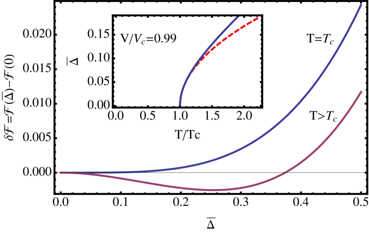
Figure 1: The difference of the canonical free energy $\delta\mathcal{F}(\bar{\Delta})$ defined in (11) is evaluated numerically keeping the density $\tilde{n}_{e}$ fixed and plotted for $V<V_{c}$ as a function of $\bar{\Delta}$ for $T=T_{c}$ and $T>T_{c}$. A clear minimum is observed as the temperature is raised above $T_{c}$ (see Eq. (15)), signifying the formation of a topological liquid phase at finite $T$. The evolution of the order parameter $\bar{\Delta}(T)$ (the location of the minimum) is shown in the inset by the solid line; the dashed line is the approximate expression for $\bar{\Delta}$ derived in (19). The filling is fixed at $\epsilon_{F}/\epsilon_{\Lambda}=\sqrt{n_{h}/n}=0.1$ and $V_{c}=1.3$.

The behavior of $\bar{\Delta}$ as $V$ crosses from $V_{c}^{-}$ to $V_{c}^{+}$ is analyzed below using Eqs. (17) and (18):

(i) For $V<V_{c}$, we fix the potential at $V=V(T_{c})$ in (17) and expand $V(T)=V(T_{c}+\delta T)$ using (18) to leading order in $\delta T/T_{c}$ and get

$$\bar{\Delta}(T)^{2}=\frac{2\pi^{2}T_{c}^{2}}{3}\left(\frac{T-T_{c}}{T_{c}}\right)\hskip 7.11317pt\textrm{as}\hskip 7.11317ptV\rightarrow V_{c}^{-}$$ (19)

A plot of this function indicated by dashed lines in the inset to Fig. 1 agrees accurately with the numerically extracted minimum (solid line in the inset) as $T\rightarrow T_{c}^{+}$.

(ii) For $V>V_{c}$, we set $T_{c}=0$ and $V=V_{c}+\delta V$ in (17). From (18) we get $V(T)/V_{c}\approx 1-(\pi V_{c}\epsilon_{F}/6)(T/\epsilon_{F})^{2}$, which when substituted in (17) gives

$$\bar{\Delta}(T)^{2}=\bar{\Delta}(0)^{2}+\frac{\pi^{2}\epsilon_{F}^{2}}{3}\left(\frac{T}{\epsilon_{F}}\right)^{2}\hskip 7.11317pt\textrm{as}\hskip 7.11317ptV\rightarrow V_{c}^{+}$$ (20)

where $\bar{\Delta}(0)^{2}=(2\pi)(\epsilon_{F}/V_{c})(\delta V/V_{c})$ gives the standard mean-field exponent of $1/2$ at $T=0$ Liu and Punnoose (2014).

(iii) Finally, at $V=V_{c}$, since $\bar{\Delta}(0)=0$ at the QCP, we get from (20) that $\bar{\Delta}(T)=\pi T/\sqrt{3}$; the linear $T$ dependence is distinct from that on either side of the QCP.

To conclude, our main observation from Eqs. (19) and (20) is that contrary to standard expectations, the intraband excitations at finite $T$ has a stabilizing effect that tend to increase $\bar{\Delta}$ as $T$ increases. The increase will eventually be limited by the interband excitations when $T\gtrsim\epsilon_{F}$, the study of which is beyond the scope of this paper. More precisely, we note from Eq. (15) that $T_{c}/\epsilon_{F}\sim\sqrt{(V_{c}-V)/\epsilon_{F}}$. Hence, provided $\delta V\ll\epsilon_{F}$, pair-breaking effects are parametrically far and our results are internally consistent with our approximations.

Finally, we want to stress the importance of studying the canonical free energy $\mathcal{F}(n_{e})$ (since the volume is held constant throughout, this translates to fixing the density), rather than directly minimizing the action $\tilde{\mathcal{L}}(\mu)$ holding $\mu$ constant. Although demanding $\partial\tilde{\mathcal{L}}/\partial\Delta=0$ recovers the saddle-point condition in (9), the condensate is unstable. To see this, we differentiate (8) twice and obtain $\partial^{2}\tilde{\mathcal{L}}/\partial\Delta^{2}=-\Delta^{2}/\Lambda<0$. This instability was pointed out earlier by us in Ref. [Liu and Punnoose, 2014] by an explicit diagrammatic calculation. In Eq. (16) we resolve this instability by showing that the mean-field condensate obtained keeping $N$ fixed, rather than $\mu$, is indeed stable.

Notice that the order parameter preserves inversion ($\mathcal{I}$) symmetry but breaks chiral ($\mathcal{C}$) symmetry in such a way that the combined $\mathcal{CT}$ symmetry is left invariant, as a result it can exhibit both anomalous Hall and Kerr effects Haldane (2004); Sun and Fradkin (2008); Castro et al. (2011). Furthermore, as noted in Ref. [Sun and Fradkin, 2008], because of the chirality, the state does not couple directly to non-magnetic impurities. Hence when spin effects can be ignored, the phase is expected to be stable. It remains to be seen, however, if the finite temperature phase described in this work survives in the presence of nearest-neighbor repulsion, which we have not included in this study.

Temperature induced topological transition has been reported in the context of thermally induced band inversion due to electron-phonon interactions Garate (2013). In our case, the topological state is induced by strong correlations and thus provides a qualitatively different paradigm involving only electronic degrees of freedom.

I appendix

II [A1] Derivation of the low temperature limit of $\mathcal{L}$

In this section, we detail the steps taken to arrive at the low temperature limit for the action $\mathcal{L}$ derived in Eq. (8). We start from the definition

$$\mathcal{L}={\varphi^{2}}/{(2V)}+\mathcal{L}_{+}+\mathcal{L}_{-}$$

where $\mathcal{L}_{\pm}$ are defined in Eq. (4). Following the discussions leading up to Eq. (8), it can be shown that the sum over $\bm{k}$ in $\mathcal{L}_{\pm}$ can be expressed as an integral with the appropriate cut-offs as

$$\mathcal{L}_{\pm}=-2T\!\int_{0}^{p_{\Lambda}}\frac{pdp}{2\pi}\ln\!\left(1+e^{-(\pm\alpha\sqrt{p^{2}+\varphi_{\lambda}^{2}}+|\mu|)/T}\right)$$

where $\mu=-|\mu|$. Substituting $z_{\pm}=(\alpha\sqrt{p^{2}+\varphi_{\lambda}^{2}}\pm|\mu|)/T$ brings the integrals into the more familiar form:

$$\mathcal{L}_{\pm}=-\frac{T^{2}}{\pi\alpha^{2}}\int\limits_{(|\Delta_{\lambda}|\pm|\mu|)/T}^{(\Lambda_{\lambda}\pm|\mu|)/T}dz\,(Tz_{\pm}\mp|\mu|)\ln(1+e^{\mp z_{\pm}})$$

The above integrals can be represented in terms of the polylogarithm functions $\textrm{Li}_{2}$ and $\textrm{Li}_{3}$. (See Ref. [24] for the definitions and properties of the polylog functions.) Rescaling $\tilde{\mathcal{L}}=(\pi\alpha^{2})\mathcal{L}$, we obtain

$$\tilde{\mathcal{L}}_{+} = \frac{\Lambda_{\lambda}^{3}}{3}-\frac{|\Delta_{\lambda}|^{3}}{3}+\frac{\Lambda_{\lambda}^{2}|\mu|}{2}-\frac{\Delta_{\lambda}^{2}|\mu|}{2}$$

$$+T^{2}\left[\Lambda_{\lambda}\textrm{Li}_{2}\left(-e^{\frac{\Lambda_{\lambda}+|\mu|}{T}}\right)-|\Delta_{\lambda}|\textrm{Li}_{2}\left(-e^{\frac{|\Delta_{\lambda}|+|\mu|}{T}}\right)\right]$$

$$-T^{3}\left[\textrm{Li}_{3}\left(-e^{\frac{\Lambda_{\lambda}+|\mu|}{T}}\right)-\textrm{Li}_{3}\left(-e^{\frac{|\Delta_{\lambda}|+|\mu|}{T}}\right)\right]$$

$$\tilde{\mathcal{L}}_{-} = T^{2}\left[\Lambda_{\lambda}\textrm{Li}_{2}\left(-e^{\frac{\Lambda_{\lambda}-|\mu|}{T}}\right)-|\Delta_{\lambda}|\textrm{Li}_{2}\left(-e^{\frac{|\Delta_{\lambda}|-|\mu|}{T}}\right)\right]$$

$$-T^{3}\left[\textrm{Li}_{3}\left(-e^{\frac{\Lambda_{\lambda}-|\mu|}{T}}\right)-\textrm{Li}_{3}\left(-e^{\frac{|\Delta_{\lambda}|-|\mu|}{T}}\right)\right]$$

To obtain the low temperature expansion, we use the asymptotic properties of the polylog functions. The required formulas to order $e^{-z}$ are listed below: (the ellipses indicate higher powers of $e^{-z}$)

$$\lim_{\textrm{Re}(z)\rightarrow\infty}\textrm{Li}_{2}(-e^{-z}) = -e^{-z}+\cdots$$

$$\textrm{Li}_{2}(-e^{z}) = -\frac{z^{2}}{2}-\frac{\pi^{2}}{6}+e^{-z}+\cdots$$

$$\textrm{Li}_{3}(-e^{-z}) = -e^{-z}+\cdots$$

$$\textrm{Li}_{3}(-e^{z}) = -\frac{z^{3}}{6}-\frac{\pi^{2}}{6}z-e^{-z}+\cdots$$

Dropping terms that fall off as $e^{-|\mu|/T}$ and higher, we get $\mathcal{L}_{+}=0$. Note that $|\Delta_{\lambda}|<E_{\lambda,F}=\sqrt{\Delta_{\lambda}^{2}+\epsilon_{F}^{2}}$ away from half-filling and $\Lambda_{\lambda}\gg\epsilon_{\lambda}$. Gathering the polynomial terms from $\tilde{\mathcal{L}}_{-}$ and substituting into $\mathcal{L}$ gives Eq. (8).

III [A2] Derivation of the Equation of State

In this section, the algebraic steps leading up to the solution for the equation of state derived in (12) are detailed. This requires solving for $\lambda$ and $\mu$ using the saddle-point equation (9) and the equation relating the chemical potential and density (10).

The relevant equations to be solved are listed below

$$\textrm{Eq. (9)}:\hskip 7.11317pt\frac{\pi\bar{\Delta}}{V} = \bar{\Delta}_{\lambda}\left(\bar{\Lambda}_{\lambda}-|\mu|\right)$$

$$\textrm{Eq.\,(10)}:\hskip 14.22636pt\mu^{2} = 2\tilde{n}_{h}+\bar{\Delta}_{\lambda}^{2}-\frac{\pi^{2}T^{2}}{3}$$

where $\Lambda_{\lambda}=\sqrt{2\tilde{n}+{\bar{\Delta}}^{2}}$. Our aim is to eliminate the square-roots from $\bar{\Lambda}_{\lambda}$ and $\mu$ and obtain a polynomial equation that can be easily solved for $\bar{\Delta}_{\lambda}$. To this end, we multiply both sides of the first equation by $(\bar{\Lambda}_{\lambda}+|\mu|)$, and use the second equation to eliminate $\mu^{2}$. This simplifies the equations to

$$\bar{\Lambda}_{\lambda}+|\mu| = \left(\frac{V}{\pi\bar{\Delta}}\right)(2\tilde{n}-2\tilde{n}_{h}+\pi^{2}T^{2}/3)\bar{\Delta}_{\lambda}$$

$$\bar{\Lambda}_{\lambda}-|\mu| = \left(\frac{\pi\bar{\Delta}}{V}\right)\frac{1}{\bar{\Delta}_{\lambda}}$$

It is now straightforward to solve for $\bar{\Delta}_{\lambda}$ by adding the two equations and squaring the result to eliminate the square-root. After some minimal algebra, we get

$$\bar{\Delta}_{\lambda}^{2}=(\bar{\Delta}+\alpha\lambda)^{2}=\left(\frac{\pi\bar{\Delta}}{V}\right)^{2}\left(\frac{(2\tilde{n}+2\tilde{n}_{h}-\pi^{2}T^{2}/3)+2\sqrt{2\tilde{n}(2\tilde{n}_{h}-\pi^{2}T^{2}/3)+(\pi\bar{\Delta}/V)^{2}}}{(2\tilde{n}-2\tilde{n}_{h}+\pi^{2}T^{2}/3)^{2}-4(\pi\bar{\Delta}/V)^{2}}\right)$$

Care must be taken in choosing the correct sign of the square-root in the numerator when solving the quadratic equation for $\bar{\Delta}_{\lambda}^{2}$. It is chosen to reproduce the solution for $V_{c}$ in Eq. (13), which can be independently obtained from the saddle-point equation in the limit $\bar{\Delta}=\lambda=0$.

Finally, we take the positive root of $\bar{\Delta}_{\lambda}^{2}$ to obtain the equation of state given in (12). This is followed by substituting the solution in the equation for $\mu^{2}$ to find $|\mu|$. The solutions for $\lambda$ and $|\mu|$ are used to obtain the exact low-temperature canonical free energy $\mathcal{F}$, defined in Eq. (11). The result for $\delta\mathcal{F}$ is plotted in Fig. 1.

References

• Haldane (1988) F. D. M. Haldane, Phys. Rev. Lett. 61, 2015 (1988).
• Mott (1961) N. F. Mott, Philos. Mag. 6, 287 (1961).
• Knox (1963) R. S. Knox, “Theory of excitons,” in Solid State Physics Suppl., Vol. 5, edited by F. Seitz and D. Turnbull (Academic Press, Inc., New York, 1963) p. 100.
• des Cloizeaux (1965) J. des Cloizeaux, J. Phys. Chem. Solids 26, 259 (1965).
• Keldysh and Kopaev (1965) L. V. Keldysh and Y. V. Kopaev, Sov. Phys. Solid State 6, 2219 (1965).
• Kozlov and Maksimov (1965) A. N. Kozlov and L. A. Maksimov, Sov. Phys. JETP 21, 790 (1965).
• Jerome et al. (1967) D. Jerome, T. M. Rice,  and W. Kohn, Phys. Rev. 158, 462 (1967).
• Halperin and Rice (1968) B. I. Halperin and T. M. Rice, Rev. Mod. Phys. 40, 755 (1968).
• Comte and Nozières (1982) C. Comte and P. Nozières, J. Phys. (Paris) 43, 1069 (1982).
• Varma (1997) C. M. Varma, Phys. Rev. B 55, 14554 (1997).
• Sun and Fradkin (2008) K. Sun and E. Fradkin, Phys. Rev. B 78, 245122 (2008).
• Liu and Punnoose (2014) W. Liu and A. Punnoose, Phys. Rev. B 89, 045126 (2014).
• Haldane (2004) F. D. M. Haldane, Phys. Rev. Lett. 93, 206602 (2004).
• Varma et al. (2002) C. M. Varma, Z. Nussinov,  and W. van Saarloos, Phys. Rep. 361, 267 (2002).
• Castro et al. (2011) E. V. Castro, A. G. Grushin, B. Valenzuela, M. A. H. Vozmediano, A. Cortijo,  and F. de Juan, Phys. Rev. Lett. 107, 106402 (2011).
• Raghu et al. (2008) S. Raghu, X.-L. Qi, C. Honerkamp,  and S.-C. Zhang, Phys. Rev. Lett. 100, 156401 (2008).
• Sun et al. (2009) K. Sun, H. Yao, E. Fradkin,  and S. A. Kivelson, Phys. Rev. Lett. 103, 046811 (2009).
• Weeks and Franz (2010) C. Weeks and M. Franz, Phys. Rev. B 81, 085105 (2010).
• Wen et al. (2010) J. Wen, A. Rüegg, C.-C. J. Wang,  and G. A. Fiete, Phys. Rev. B 82, 075125 (2010).
• Tieleman et al. (2013) O. Tieleman, O. Dutta, M. Lewenstein,  and A. Eckardt, Phys. Rev. Lett. 110, 096405 (2013).
• Kurita et al. (2013) M. Kurita, Y. Yamaji,  and M. Imada, Phys. Rev. B 88, 115143 (2013).
• Grushin et al. (2013) A. G. Grushin, E. V. Castro, A. Cortijo, F. de Juan, M. A. H. Vozmediano,  and B. Valenzuela, Phys. Rev. B 87, 085136 (2013).
• Durić et al. (2014) T. Durić, N. Chancellor,  and I. F. Herbut, Phys. Rev. B 89, 165123 (2014).
• Tinkham (1992) M. Tinkham, Group Theory and Quantum Mechanics (Dover Publications, New York, 1992).
• de Gennes (1963) P. G. de Gennes, Solid State Commun. 1, 132 (1963).
• Brout et al. (1966) R. Brout, K. A. Müller,  and H. Thomas, Solid State Commun. 4, 507 (1966).
• Imada et al. (2010) M. Imada, T. Misawa,  and Y. Yamaji, J. Phys.: Condens. Matter 22, 164206 (2010).
• Altland and Simons (2010) A. Altland and B. Simons, Condensed Matter Field Theory, 2nd ed. (Cambridge Univeristy Press, 2010).
• Abrikosov et al. (1975) A. A. Abrikosov, L. P. Gorkov,  and I. E. Dzyaloshinski, Methods of Quantum Field Theory in Statistical Physics (Dover Publications, New York, 1975).
• Note (1) The TMI has been analyzed in detail in Ref. [\rev@citealpimada_gapless]; the deviation from the standard LGW theory, peculiar to the half-filled case at $T=0$, vanish both at finite $T$ and/or doping. For the interested reader, the relationship between the parameters in [\rev@citealpimada_gapless] with those in this paper are: $\zeta=\varphi/V,\tmspace+{.1667em}\Lambda=p_{\Lambda},\tmspace+{.1667em}t=\alpha/\sqrt{3}$ and $V_{2}/t=V/3$.
• Abramowitz and Stegun (1964) M. Abramowitz and I. A. Stegun, eds., Handbook of Mathematical Functions (National Bureau of Standards, Washington, DC, 1964).
• Negele and Orland (1998) J. W. Negele and H. Orland, Quantum many-particle systems (Perseus Books, Massachusetts, 1998).
• Garate (2013) I. Garate, Phys. Rev. Lett. 110, 046402 (2013).