Quantum Isothermal Reversible Process of Particles in a Box with a Delta Potential

Abstract

For an understanding of a heat engine working in the microscopic scale, it is often necessary to estimate the amount of reversible work extracted by isothermal expansion of the quantum gas used as its working substance. We consider an engine with a movable wall, modeled as an infinite square well with a delta peak inside. By solving the resulting one-dimensional Schrödinger equation, we obtain the energy levels and the thermodynamic potentials. Our result shows how quantum tunneling degrades the engine by decreasing the amount of reversible work during the isothermal expansion.

I Introduction

A fundamental idea behind classical statistical mechanics is that we are living in a macroscopic world, which means that we are unable to deal with microstates on a molecular level. This forces us to distinguish heat from work and to accept the increase of entropy on probabilistic ground, when we formulate the laws of thermodynamics. However, the border between our macroscopic world and the microscopic world of molecules is becoming vague due to technological developments over the last century. This has led to a natural question; i.e., what would it mean to thermodynamics if it became possible to access and manipulate microstates just as we do macrostates? The founders of statistical mechanics were already aware of this problem: For example, Maxwell imagined an intelligent being’s intervention on a molecular level in his famous thought experiment, now known as Maxwell’s demon Maruyama et al. (2009), and expressed deep concern about the foundation of the second law of thermodynamics.

The Szilard engine has been regarded as the simplest implementation of Maxwell’s demon with a single-particle gas Sagawa and Ueda (2013). Its cycle consists of four processes; inserting a wall into the center of the box, measuring the position of the particle, expanding the quantum gas isothermally, and finally removing the wall. Considering its microscopic nature, it is tempting to translate the cycle into quantum-mechanical language as has been done in Refs. Bender et al., 2000 and Kieu, 2004 for other engines. In fact, there are more reasons than that: Zurek Zurek (1986), when he discusses Jauch and Baron’s objection that the gas is compressed without the expenditure of energy upon inserting the wall, argues that one has to resort to quantum mechanics to understand the Szilard engine Jauch and Baron (1972). According to Ref. Zurek, 1986, this ‘apparent inconsistency’ is removed by quantum-mechanical considerations. Therefore, in a sense, it is a matter of theoretical consistency. Kim and coworkers have presented a detailed account for its quantum-mechanical cycle in Refs. Kim et al., 2011; Kim and Kim, 2011, 2012, with emphasis on the isothermal process. There seem to remain some subtle issues to settle, however, as shown in the debate on how to deal with the quantum tunneling effect through the wall in a three-boson case Plesch et al. (2013).

In this work, we describe the isothermal expansion of the quantum Szilard engine by considering a quantum gas confined in a one-dimensional cylinder Vugalter et al. (2002); Pedram and Vahabi (2010). Although some previous studies, such as Refs. Bender et al., 2005; Dong et al., 2011; Li et al., 2012, assume that the wall is impenetrable, we will relax that assumption because it is, strictly speaking, experimentally infeasible. Starting from the Schrödinger equation, we calculate the energy levels and thereby obtain how much work can be extracted by an isothermal reversible expansion. We find the following: The amount of reversible work is significantly reduced compared to the claims in Refs. Zurek, 1986 and Kim et al., 2011 if we assume full thermal equilibrium inside the box, as is usual in describing isothermal expansion. This conclusion should not be affected by either the wall’s insertion or the measurement before the isothermal expansion because thermal equilibrium does not remember its history. Moreover, if we put two or three fermions in the box, the free-energy landscape is not monotonic with respect to the wall’s position, so that we should sometimes perform work to expand the gas. These effects have not been explicitly discussed in previous studies.

This work is organized as follows: An explanation of our basic setting in terms of the Schrödinger equation is given in Section II. A numeric calculation of the energy levels and the free energy and a comparison of a single-particle case to the two- and three-particle cases is presented in in Section III. This is followed by discussion of results and conclusions.

II Particle in a box

Consider the following one-dimensional potential landscape with size $L$:

$$V(x)=\left\{\begin{array}[]{lc}a\delta(x-pL)&\mbox{if~{}}0<x<L\\ \infty&\mbox{elsewhere},\end{array}\right.$$ (1)

where $a$ is the strength of the delta potential and $p\in(0,1)$ specifies its location Griffiths (1995). We expect the Schrödinger equation

$$\left[-\frac{\hbar^{2}}{2m}\frac{d^{2}}{dx^{2}}+V(x)\right]\psi(x)=E\psi(x)$$ (2)

to have a solution with a sinusoidal form. The boundary conditions at $x=0$ and $x=L$ are satisfied if we set

$$\psi(x)=\left\{\begin{array}[]{lc}A\sin kx&\mbox{if~{}}0<x<pL\\ B\sin k(L-x)&\mbox{if~{}}pL<x<L,\\ \end{array}\right.$$ (3)

where the coefficients $A$ and $B$, as well as the wavenumber $k$, are assumed to be nonzero. The eigenfunction $\psi(x)$ has the following properties: First, it is continuous over $[0,L]$; i.e.,

$$A\sin pkL=B\sin qkL$$ (4)

with $q\equiv 1-p$. Second, the change in the derivative of $\psi(x)$ with respect to $x$ around $x=pL$ is obtained by using

$$\lim_{\epsilon\rightarrow 0}\left\{\int_{pL-\epsilon}^{pL+\epsilon}\left[\frac{d^{2}}{dx^{2}}\psi(x)\right]dx+\frac{2m}{\hbar^{2}}\left[\int_{pL-\epsilon}^{pL+\epsilon}E\psi(x)dx-\int_{pL-\epsilon}^{pL+\epsilon}a\psi(x)\delta(x-pL)dx\right]\right\}=0,$$ (5)

from which it follows that

$$\lim_{\epsilon\rightarrow 0}\left(\left.\frac{d\psi}{dx}\right|_{pL+\epsilon}-\left.\frac{d\psi}{dx}\right|_{pL-\epsilon}\right)=\frac{2ma}{\hbar^{2}}\psi(pL).$$ (6)

Plugging Eq. (3) here and multiplying both sides by $\sin qkL$ to use Eq. (4), we obtain

$$-k\sin kL=\frac{2ma}{\hbar^{2}}\sin pkL\sin qkL.$$ (7)

This formula has also been derived in Ref. Pedram and Vahabi, 2010 in a different way. Equation (7) can be numerically solved by using the Newton-Raphson method to yield the allowed values of $k$. The method works as follows: First, let us define $f(k)\equiv k\sin kL+\frac{2ma}{\hbar^{2}}\sin pkL\sin qkL$, and look for its zeros to solve Eq. (7). Starting from $k=0$, we check whether the sign of $f(k)$ changes with increasing $k$ by a sufficiently small amount, say, $dk\ll 1$. Every time the sign changes between $k=k^{\ast}>0$ and $k^{\ast}+dk$, we run the following iteration starting from $k^{(0)}=k^{\ast}$:

$$k^{(j+1)}=k^{(j)}-\frac{f[k^{(j)}]}{f^{\prime}[k^{(j)}]},$$ (8)

where $j=0,1,2,\ldots$. When $k^{(j)}$ has converged to a stationary value $k^{(\infty)}$, i.e., if $k^{(j)}=k^{(j+1)}$ within numerical accuracy, we take it as a solution of Eq. (7) and repeat the procedure by checking the sign of $f(k)$ from $k=k^{(\infty)}+dk$. Each of these solutions is identified with the wavenumber $k_{n}$ of the $n$th eigenmode in an ascending order. For the application of the Newton-Raphson method numerically, it is convenient to express the quantities in dimensionless units, so we divide Eq. (2) by $E^{(0)}_{g}\equiv\hbar^{2}\pi^{2}/(2mL^{2})$, the ground state energy for $a=0$, to obtain

$$\left[\frac{d}{d\eta^{2}}\psi(\eta)+\Phi(\eta)\right]\psi(\eta)=\epsilon\psi(\eta),$$ (9)

where $\eta\equiv\pi x/L$. Then, the potential inside the box is expressed as

$$\Phi(\eta)=\frac{2mL^{2}}{\hbar^{2}\pi^{2}}a\delta(x-pL)=\alpha\delta(\eta-p\pi),$$ (10)

with $\alpha\equiv 2amL/(\hbar^{2}\pi)=a(L/\pi)/E^{(0)}_{g}$. We can also define a dimensionless wavenumber $\kappa\equiv Lk/\pi$ to rewrite Eqs. (7) as $\kappa\sin\kappa\pi+\alpha\sin p\kappa\pi\sin q\kappa\pi=0$. A little algebra shows that the energy level is given by

$$\epsilon=\kappa^{2}+\frac{2\alpha}{\pi}\left[\csc^{2}p\kappa\pi\left(p-\frac{1}{2\kappa\pi}\sin 2p\kappa\pi\right)+\csc^{2}q\kappa\pi\left(q-\frac{1}{2\kappa\pi}\sin 2q\kappa\pi\right)\right]^{-1},$$ (11)

where the second term represents the potential energy coming from the overlap between the wavefunction and the delta peak potential. The numerical solutions for these $\kappa$ and $\epsilon$ are depicted in Fig. 1, together with the probability density plots.

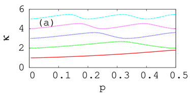
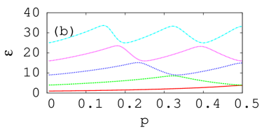
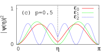
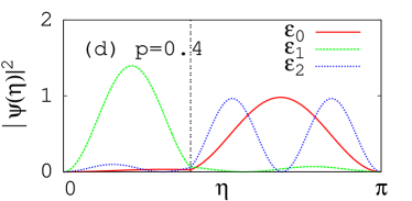
Figure 1: (Color online) (a) Lowest wavenumbers in units of $\pi/L$ as a function of $p$, and (b) the corresponding energy levels in units of $E^{(0)}_{g}=\hbar^{2}\pi^{2}/(2mL^{2})$. The other two panels show the probability densities for the three lowest eigenmodes (c) when the wall is in the middle, $p=0.5$, and (d) when it has moved to $p=0.4$. The strength of the potential is set as $\alpha=10$.

III Reversible work

III.1 Single Particle

We are interested in how much work can be extracted by performing a reversible isothermal process with this system. Let $\epsilon_{n}$ denote the $n$th energy level obtained by using the Newton-Raphson method with $n=1,\ldots,M$ so that the ground-state energy is denoted by $\epsilon_{1}$. For a given value of temperature $T=(k_{B}\beta)^{-1}$, where $k_{B}$ is the Boltzmann constant, we run the calculation to get $\beta\epsilon_{M}\gg 1$. The partition function for a single quantum particle can then be obtained as

$$Z=\lim_{M\rightarrow\infty}\sum_{n=1}^{M}e^{-\beta\epsilon_{n}}.$$ (12)

The free energy is $F=-k_{B}T\ln Z$, accompanied by a differential form $dF=-SdT-PdV$, where $S$, $P$, and $V$ are the entropy, pressure, and volume, respectively. The classical concepts, such as pressure and work, need careful consideration in quantum mechanics Borowski et al. (2003). To calculate work, we begin with the occupation probability of the $n$th level given by

$$\rho_{n}=\frac{e^{-\beta\epsilon_{n}}}{\sum_{n}e^{-\beta\epsilon_{n}}}=\frac{-k_{B}T\left(\partial Z/\partial\epsilon_{n}\right)}{Z}=\frac{\partial}{\partial\epsilon_{n}}(-k_{B}T\ln Z)=\frac{\partial F}{\partial\epsilon_{n}}.$$ (13)

The change in the internal energy $U=\sum_{n}\rho_{n}\epsilon_{n}$ is then expressed as $dU=\sum_{n}\epsilon_{n}d\rho_{n}+\rho_{n}d\epsilon_{n}={\mathchar 22\relax\mkern-11.0mu\mathrm{d}}Q+{\mathchar 22\relax\mkern-11.0mu\mathrm{d}}W$, where ${\mathchar 22\relax\mkern-11.0mu\mathrm{d}}Q$ and ${\mathchar 22\relax\mkern-11.0mu\mathrm{d}}W$ are differentials of heat and work, respectively. The quantum thermodynamic work is identified with ${\mathchar 22\relax\mkern-11.0mu\mathrm{d}}W=\sum_{n}\rho_{n}d\epsilon_{n}$ because heat is usually involved with changes in occupation probabilities for given energy levels whereas work is performed when the energy levels themselves change Kim et al. (2011) . Consequently, the amount of reversible work during this process is $W=\int\sum_{n}\frac{\partial F}{\partial\epsilon_{n}}d\epsilon_{n}=\int dF=\Delta F$, which is consistent with the classical case.

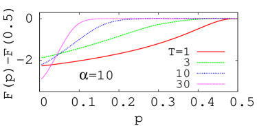
Figure 2: (Color online) Change in the free energy $F$ in units of $E^{(0)}_{g}=\hbar^{2}\pi^{2}/(2mL^{2})$ when the wall, starting from the center of the box, moves to a new position $p$. The height of the wall is fixed at $\alpha=10$, and each curve represents a different $T$ in units of $E^{(0)}_{g}/k_{B}$. The number of energy levels considered is kept as $M=10^{3}$ throughout the free-energy calculations.

Figure 2 shows $\Delta F$ resulting from moving the wall, which was initially located at the center, $p=0.5$. Suppose that $T$ is so low that $T\lesssim E^{(0)}_{g}/k_{B}$. When the wall is at $p=0$, only the ground state contributes to the summation in Eq. (12), which means that $Z(p=0)\approx e^{-\beta E^{(0)}_{g}}$. When the wall is at $p=0.5$, the ground-state energy equals $4E^{(0)}_{g}$, and the first excited state also contributes to the partition sum in Eq. (12) because it lies close to the ground state [see Fig. 1(b)]. The partition function is, therefore, approximated as $Z(p=0.5)\approx 2e^{-4\beta E^{(0)}_{g}}$. The free-energy difference in this low-$T$ region is, thus, given as $F(0)-F(0.5)\approx-3E^{(0)}_{g}+k_{B}T\ln 2$. When $T=E^{(0)}_{g}/k_{B}$, for example, the free-energy difference roughly amounts to $-2.3E^{(0)}_{g}$, which explains the size of the free-energy drop in Fig. 2.

As $T$ increases, a plateau develops near the center of the box because $F$ does not respond much to the wall’s position. However, the drop in $F$ at the end of the process increases with increasing $T$ if $T\gg O(1)$ in units of $E^{(0)}_{g}/k_{B}$. Our question is how it grows with $T$. Let us take $\alpha\rightarrow\infty$ and $\gamma\equiv\beta\hbar^{2}\pi^{2}/(2mL^{2})\ll 1$. Then, it is the partition function for the initial and final wall positions can be approximated. The latter case of the final wall position is estimated as

$$Z(p=0) = \sum_{n=1}^{\infty}e^{-\gamma n^{2}}$$ (14)

$$\approx \int_{0}^{\infty}\exp(-\gamma n^{2})dn-\frac{1}{2}\sum_{n=0}^{\infty}\left[e^{-\gamma n^{2}}-e^{-\gamma(n+1)^{2}}\right]$$ (15)

$$= \sqrt{\frac{\pi}{4\gamma}}-\frac{1}{2},$$ (16)

where the summation in Eq. (15) is a first-order correction to the integral approximation. Likewise, the former case of the initial wall position gives

$$Z(p=0.5)=2\sum_{n=1}^{\infty}e^{-4\gamma n^{2}}\approx 2\left[\int_{0}^{\infty}\exp(-4\gamma n^{2})dn-\frac{1}{2}\right]=\sqrt{\frac{\pi}{4\gamma}}-1,$$ (17)

where the factor of $2$ in front of the summation is due to the fact that every pair of adjacent energy levels becomes degenerate in the limit of $\alpha\rightarrow\infty$. This effect cancels the factor of $4$ inside the exponential arising from the reduced volume $L/2$. Although $\Delta F$ does not completely vanish due to the correction, the important point is that $Z(0.5)/Z(0)$ for $\gamma\ll 1$ is far less than $2$, in contrast with the claim that $\Delta F=-k_{B}T\ln 2$ in Refs. Zurek, 1986 and Kim et al., 2011. Because $\alpha$ must be finite in any experimental situation, the particle can, in full thermal equilibrium, be observed on either side of the box, which reduces the amount of extracted work. On the other hand, the previous studies on the quantum Szilard engine Zurek (1986); Kim et al. (2011) have assumed that the process is performed within a shorter time scale than required for tunneling through the wall and, therefore, concluded that $Z(p=0.5)\approx\int\exp(-4\gamma n^{2})dn$ without the factor of $2$ in front. Strictly speaking, their engine undergoes an isothermal process only when partially equilibrated to maintain the confinement and extract $W=k_{B}T\ln 2$.

III.2 Two- and Three-particle Cases

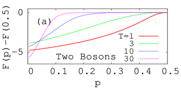
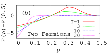
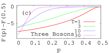
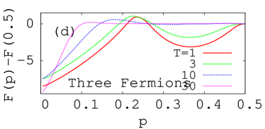
Figure 3: (Color online) Free-energy changes in the presence of multiple non-interacting quantum particles: (a) bosonic and (b) fermionic cases with two particles. With three particles, (c) the bosonic case remains qualitatively similar, but (d) the fermions behave differently due to the Pauli exclusion principle.

If two quantum particles are in the box, we should consider their symmetry, i.e., whether they are fermions or bosons. Without any consideration of the spin degree of freedom, the elements of the density matrix for the two particles are expressed in the bracket notation as follows: $\left<\epsilon_{1}^{\prime}\epsilon_{2}^{\prime}\left|e^{-\beta\hat{H}}\right|\epsilon_{1}\epsilon_{2}\right>=e^{-\beta(\epsilon_{1}+\epsilon_{2})}\left(\delta_{\epsilon_{1}^{\prime}\epsilon_{1}}\delta_{\epsilon_{2}^{\prime}\epsilon_{2}}\pm\delta_{\epsilon_{1}^{\prime}\epsilon_{2}}\delta_{\epsilon_{2}^{\prime}\epsilon_{1}}\right)$, where $\delta$ is the Kronecker delta symbol, and we have a plus sign for bosons and a minus sign for fermions. The two-particle partition function is then obtained by taking the trace operation:

$$Z=\text{Tr}\left(e^{-\beta\hat{H}}\right)=\frac{1}{2!}\sum_{\epsilon_{1},\epsilon_{2}}e^{-\beta(\epsilon_{1}+\epsilon_{2})}\left(1\pm\delta_{\epsilon_{1}\epsilon_{2}}\right).$$ (18)

The same applies to the three-particle case. The density-matrix elements are written as $\left<\epsilon_{1}^{\prime}\epsilon_{2}^{\prime}\epsilon_{3}^{\prime}\left|e^{-\beta\hat{H}}\right|\epsilon_{1}\epsilon_{2}\epsilon_{3}\right>=e^{-\beta(\epsilon_{1}+\epsilon_{2}+\epsilon_{3})}\left(\delta_{\epsilon_{1}^{\prime}\epsilon_{1}}\delta_{\epsilon_{2}^{\prime}\epsilon_{2}}\delta_{\epsilon_{3}^{\prime}\epsilon_{3}}\pm\ldots\right)$, and the partition function reads

$$Z=\text{Tr}\left(e^{-\beta\hat{H}}\right)=\frac{1}{3!}\sum_{\epsilon_{1},\epsilon_{2},\epsilon_{3}}e^{-\beta(\epsilon_{1}+\epsilon_{2}+\epsilon_{3})}\left(1\pm\delta_{\epsilon_{1}\epsilon_{2}}\pm\delta_{\epsilon_{2}\epsilon_{3}}\pm\delta_{\epsilon_{3}\epsilon_{1}}+2\delta_{\epsilon_{1}\epsilon_{2}}\delta_{\epsilon_{2}\epsilon_{3}}\right).$$ (19)

Figure 3 shows the free-energy differences for the two- and the three-particle cases. The bosonic cases are qualitatively similar to the single-particle case. However, we see very different behavior for the fermionic cases where the Pauli exclusion principle is in action: At low $T$, we need to perform positive work to move the wall from the center to a certain position $p$ [Figs. 3(b) and (d)]. Obviously, the reason is that it costs free energy to place two fermions close to each other.

IV Summary and Outlook

In summary, we have considered an isothermal expansion process of a quantum gas, taking the tunneling effect into consideration. We have found that the amount of reversible work is smaller than $k_{B}T\ln 2$ in the high-$T$ region if the system is fully equilibrated at every moment of the isothermal expansion. The difference from Refs. Zurek, 1986 and Kim et al., 2011 arises because they have separated the time scale of tunneling from that of the partial equilibration that occurs on only one side of the wall. Although it was not explicitly stated in previous studies, this separation may be a plausible assumption for the following reason: As we increase the potential height $\alpha$, we may well expect the time scale for tunneling to grow whereas the partial equilibration before tunneling is achieved within a finite amount of time. The quantum Szilard engine will show its expected performance only between these two time scales. The question is, then, how large a value of $\alpha$ one should have to ensure the separation of the time scales, which will be pursued in our future studies.