Local Orthogonal Polynomial Expansion for Density Estimation

Abstract

A Local Orthogonal Polynomial Expansion (LOrPE) of the empirical density function is proposed as a novel method to estimate the underlying density. The estimate is constructed by matching localized expectation values of orthogonal polynomials to the values observed in the sample. LOrPE is related to several existing methods, and generalizes straightforwardly to multivariate settings. By manner of construction, it is similar to Local Likelihood Density Estimation (LLDE). In the limit of small bandwidths, LOrPE functions as Kernel Density Estimation (KDE) with high-order (effective) kernels inherently free of boundary bias, a natural consequence of kernel reshaping to accommodate endpoints. Faster asymptotic convergence rates follow. In the limit of large bandwidths, LOrPE is equivalent to Orthogonal Series Density Estimation (OSDE) with Legendre polynomials. We compare the performance of LOrPE to KDE, LLDE, and OSDE, in a number of simulation studies. In terms of mean integrated squared error, the results suggest that with a proper balance of the two tuning parameters, bandwidth and degree, LOrPE generally outperforms these competitors when estimating densities with sharply truncated supports.

Keywords: boundary bias; kernel density estimation; local likelihood density estimation; mean integrated squared error; orthogonal series density estimation; sharply truncated support.

1 Introduction

Few areas of statistical inference receive as much attention as the classical problem of nonparametric density estimation. Taking as our basis for inference a random sample of observations $x_{1},\ldots,x_{n}$ from an underlying continuous distribution with probability density function (PDF) $f(\cdot)$ defined on the compact support $[a,b]$, the simplest starting point is the empirical density function (EDF)

$$\hat{f}_{\text{EMP}}(x)=\frac{1}{n}\sum_{i=1}^{n}\delta(x-x_{i}),$$ (1)

where $\delta(\cdot)$ is the Dirac delta function. If additionally we assume the existence of a first few derivatives or that the PDF can have at most a few modes, a convolution of the EDF with a kernel function, $K(\cdot)$, often provides a much better estimate by producing a weighted average of points close to $x$. $K(\cdot)$ itself is usually chosen to be a symmetric continuous density with a scale parameter, so that the resulting kernel density estimate (KDE) is

$$\hat{f}_{\text{KDE}}(x)\equiv\int\frac{1}{h}K\left(\frac{x-y}{h}\right)\hat{f}_{\text{EMP}}(y)dy=\frac{1}{n}\sum_{i=1}^{n}\frac{1}{h}K\left(\frac{x-x_{i}}{h}\right).$$ (2)

The critical KDE tuning parameter is the bandwidth $h$. A convenient, tractable criterion which is typically used to optimize the choice of this parameter is the mean integrated squared error (MISE). For large sample sizes, the MISE can be expanded in powers of $n^{-1}$. The two leading terms in this expansion are associated with the bias and variance of the estimator. Omission of all higher-order terms results in the asymptotic MISE (AMISE) approximation.

Under regularity conditions, KDE is consistent, with an AMISE-optimal choice of bandwidth ($h_{\ast}$) which depends on (computable) kernel moments and the (uncomputable) integrated squared curvature of $f$. Although the Epanechnikov kernel minimizes AMISE (is asymptotically optimal), the choice of kernel is generally not as influential as the choice of bandwidth. See Silverman (1986), Scott (1992) and Wand & Jones (1995) for detailed treatments of the subject, and Sheather (2004), Wasserman (2006, ch. 6), and Givens & Hoeting (2013, ch. 10) for more concise surveys.

Although the optimal $h_{\ast}$ is unattainable in practice, there are several approaches to dealing with this issue. They range from quick rules-of-thumb, or plug-in methods, to the more computationally-intensive bandwidth selection based on cross-validation (Heidenreich et al., 2013). Rather, the major drawback of KDE is that it suffers from boundary bias, particularly if $f$ is sharply truncated at the edges of its support. In such bounded support settings, KDE fails to attain the optimal convergence rate (Jones, 1993).

One of the earliest attempts at correcting this problem was truncation and reflection of boundary kernels (Silverman, 1986). Several solutions based on local or adaptive methods have since been proposed; see for example Malec & Schienle (2014) for a survey. A more general solution is to use a local polynomial or local likelihood based approach (Hjort & Jones, 1996, Loader, 1996, 1999). These methods, and in particular the local likelihood density estimation (LLDE) detailed in Loader (1999), alleviate boundary bias, but require the solution of nonlinear equations at each $x$, and are therefore slow to compute. (Hall & Tao, 2002, however, argue that KDE has distinct advantages over LLDE in the absence of boundary effects.) Although adaptive kernels work fairly well (e.g., Chen, 1999, Kakizawa, 2004, Jones & Henderson, 2007), they presume some particular number of derivatives is matched at the boundary, which affects their asymptotic performance.

There is thus a niche to be filled in the nonparametric density estimation literature by devising methods that alleviate the boundary bias issues in a more general way than the prescribed corrections of adaptive methods, whilst attaining the optimal KDE convergence rates in the interior of the support, and yet do all this in a computationally efficient manner. As will be argued, our proposed method attains faster asymptotic convergence rates by virtue of using higher-order (effective) kernels. The initial motivation for our quest comes from high energy physics experiments, where there is a need to estimate the distribution of visible energy in jets (i.e., collections of particles moving in approximately the same direction) due to smearing by the detector resolution (Volobouev, 2011). The situation is complicated by the fact that the energy of any one jet has to be reconstructed from signals produced by multiple particles in an array of sensors in the measuring device (calorimeter) with non-linear response (Wigmans, 2000).

It is sometimes possible to use parametric functions to model such distributions. The results are fair, but there is room for improvement. Borrowing from the methods in Thas (2010), one idea is to model the bulk of the distribution with a flexible parametric model (like Johnson curves, Elderton & Johnson, 1969), and describe the deviations from this model nonparametrically, in the spirit of Yang & Marron (1999). This can be done with so called ”comparison distributions” (Thas, 2010, ch. 3). The basic approach is that if $g$ and $G$ denote respectively the PDF and cumulative distribution function (CDF) of a generic member of the parametric Johnson curves, and if $\psi$ and $\Psi$ denote the PDF and CDF of a distribution supported on $[0,1]$, then $F(x)=\Psi(G(x))$ is also a CDF, with

$$f(x)=g(x)\psi(G(x)),$$ (3)

as its corresponding PDF. (This procedure can be iterated given a sequence of CDFs $\{\Psi_{1},\Psi_{2},\ldots\}$ supported on $[0,1]$.)

This suggests one can model observations $\{x_{i}\}$ from $X\sim f$ by first approximating $f$ with $g$, even if it proves to be somewhat inadequate, and then mapping the $\{x_{i}\}$ to the $[0,1]$ interval according to the transformation, $y_{i}=G(x_{i})$. The density of the $\{y_{i}\}$ can now be approximated, either parametrically or nonparametrically, to yield an estimate of $\psi$, whence the final $f$ is obtained from (3). In the case that $G=F$, the true CDF, we have of course that $G(X)$ is uniform on $[0,1]$, a fact which can be used to assess the appropriateness of the initial $G$ (e.g., via the comparison distribution methodology outlined in Thas, 2010, ch. 3). This is precisely where improved versions of KDE come in; they are needed to handle the sharply truncated support boundaries of the density of the $\{y_{i}\}$ resulting from this approach.

In multivariate problems, an attractive density estimation approach consists in decomposing the estimated density into the product of the copula density and of the marginals (Gijbels & Mielniczuk, 1990). As the copula density is defined on the unit hypercube, KDE of the copula density suffers considerably from boundary bias. While a number of methods have been proposed for alleviating this deficiency (as reviewed in Charpentier et al., 2006; see also Chen & Huang, 2007), the asymptotic convergence rate of these methods at the boundary is nevertheless inferior to the convergence rate inside the hypercube.

With this backdrop, we propose the use of local orthogonal polynomial expansion (LOrPE) as a new method to perform nonparametric density estimation. The theoretical development and genesis of LOrPE is discussed in section 2. Section 3 discusses connections with other methods: KDE, LLDE, and orthogonal series density estimation (OSDE). In particular, we establish there that LOrPE is equivalent to KDE with a high-order kernel for points well inside the support of the PDF. Thus, and through appropriate choice of its tuning parameters (discussed in section 4), LOrPE provides a general way to achieve adaptive (kernel) behavior, while also attaining optimal asymptotic convergence rates. Section 5 examines the performance of LOrPE closely in some simulation studies, in both oracle (best case) and non-oracle settings, with respect to the competitors outlined in section 3. The paper concludes in section 6 with an illustration on a real dataset.

2 Development of LOrPE

LOrPE inherits several of its features from OSDE (Efromovich, 1999), and can in fact be thought of as a localized version of OSDE. With $\hat{f}(x)$ a simple initial estimator such as (1), LOrPE amounts to constructing a truncated orthogonal polynomial series expansion for the EDF near each point $x_{\mbox{\scriptsize\,fit}}$ where the density estimate is desired. (In practice, these points would usually be taken to be uniformly spaced on a grid of values covering the support of the density.) For a chosen bandwidth $h$, this expansion is

$$\tilde{f}_{\text{LOrPE}}(x)=\sum_{k=0}^{M}c_{k}(x_{\mbox{\scriptsize\,fit}},h)P_{k}\left(\frac{x-x_{\mbox{\scriptsize\,fit}}}{h}\right),$$ (4)

where the polynomials $P_{k}(x)$ are constrained to satisfy the normalization condition

$$\frac{1}{h}\int_{a}^{b}P_{j}\left(\frac{x-x_{\mbox{\scriptsize\,fit}}}{h}\right)P_{k}\left(\frac{x-x_{\mbox{\scriptsize\,fit}}}{h}\right)K\left(\frac{x-x_{\mbox{\scriptsize\,fit}}}{h}\right)dx=\delta_{jk},$$ (5)

which, with $\tilde{a}_{\mbox{\scriptsize\,fit}}=(a-x_{\mbox{\scriptsize\,fit}})/h$ and $\tilde{b}_{\mbox{\scriptsize\,fit}}=(b-x_{\mbox{\scriptsize\,fit}})/h$, is equivalent to

$$\int_{\tilde{a}_{\mbox{\scriptsize\,fit}}}^{\tilde{b}_{\mbox{\scriptsize\,fit}}}P_{j}(y)P_{k}(y)K(y)dy=\delta_{jk},$$ (6)

where $\delta_{jk}$ is the Kronecker delta and $K(\cdot)$ a suitably chosen kernel function. The coefficients $c_{k}(x_{\mbox{\scriptsize\,fit}},h)$ are determined by

$$c_{k}(x_{\mbox{\scriptsize\,fit}},h)=\frac{1}{h}\int\hat{f}(x)P_{k}((x-x_{\mbox{\scriptsize\,fit}})/h)K((x-x_{\mbox{\scriptsize\,fit}})/h)dx,$$ (7)

which, for $\hat{f}(x)=\hat{f}_{\text{EMP}}(x)$, is equivalent to

$$c_{k}(x_{\mbox{\scriptsize\,fit}},h)=\frac{1}{nh}\sum_{i=1}^{n}P_{k}((x_{i}-x_{\mbox{\scriptsize\,fit}})/h)K((x_{i}-x_{\mbox{\scriptsize\,fit}})/h).$$ (8)

Because negative values can occur, the proposed density estimate at $x=x_{\mbox{\scriptsize\,fit}}$ is then $\max\{0,\tilde{f}_{\text{LOrPE}}(x_{\mbox{\scriptsize\,fit}})\}$. In general, this does not result in a bona fide density function (similarly to OSDE), and thus the final step in the process involves performing a renormalization over all grid points. The final (genuine) density estimate at $x$ is denoted by $\hat{f}_{\text{LOrPE}}(x)$. Generalizing LOrPE to a multivariate setting is in principle straightforward, necessitating only a switch to multivariate orthogonal polynomial systems.

Equation (4) can be usefully generalized to include a taper function $t(k)$ as follows:

$$\tilde{f}_{\text{LOrPE}}(x)=\sum_{k=0}^{\infty}t(k)c_{k}(x_{\mbox{\scriptsize\,fit}},h)P_{k}((x-x_{\mbox{\scriptsize\,fit}})/h).$$ (9)

The idea of the taper function is to suppress high order terms gradually, instead of using a sharp cutoff at $M$. Also, as will be discussed in section 4, a particular definition of the taper function allows for a simple extension of (4) to non-integer values of $M$. We will normally require that $t(0)=1$ in order to ensure correct asymptotic normalization, in addition to specifying that $t(k)=0$ for $k>M$.

LOrPE admits an appealing interpretation in terms of the local density expansion (4), in which the “localized” expectation values of the orthogonal polynomials $P_{k}(\cdot)$ are matched to their empirical values calculated from the data sample. This heuristic interpretation can be understood by making the following observation. Define the localized expectation (at $x_{\mbox{\scriptsize\,fit}}$) of a function $\phi$ with respect to kernel $K$ (bandwidth $h$) for a random variable $X\sim f$ as,

$$\mathbb{E}^{(\text{loc})}_{f}[\phi(X)]=\frac{\int\phi(x)K(x)f(x)dx}{\int K(x)f(x)dx}.$$

Then, upon setting $\phi(x)=P_{k}(x)$, note that

$$\mathbb{E}^{(\text{loc})}_{\hat{f}_{\text{EMP}}}[P_{k}(X)]=\frac{c_{k}(x_{\mbox{\scriptsize\,fit}},h)}{c_{0}(x_{\mbox{\scriptsize\,fit}},h)}=\mathbb{E}^{(\text{loc})}_{\tilde{f}_{\text{LOrPE}}}[P_{k}(X)].$$

3 Connections With Other Methods

This section explores the connections between LOrPE and KDE, OSDE, and LLDE. We will show that under certain conditions LOrPE is essentially equivalent to KDE (Theorem 1); while under other conditions its behavior mimics OSDE (Theorem 2). Also, the local adjustments instituted by LOrPE to reduce support boundary bias are very much in the spirit of LLDE.

3.1 Kernel density estimation

In general, LOrPE behaves as a linear combination of KDEs with varying kernels. To see this, define $K_{k}(z)=P_{k}(z)K(z)$, and note that from (7) with $\hat{f}(x)=\hat{f}_{\text{EMP}}(x)$ we can write the expansion coefficients as

$$c_{k}(x_{\mbox{\scriptsize\,fit}},h)=\int\frac{1}{h}K_{k}\left(\frac{x-x_{\mbox{\scriptsize\,fit}}}{h}\right)\hat{f}_{\text{EMP}}(x)dx\equiv\hat{f}_{\text{KDE}}(x|h,K_{k}),$$

where the notation $\hat{f}_{\text{KDE}}(x|h,K)$ emphasizes the dependence on bandwidth $h$ and kernel $K$. Thus (4) can be written as a weighted linear combination of KDEs with varying (improper) kernels $K_{k}$,

$$\tilde{f}_{\text{LOrPE}}(x)=\sum_{k=0}^{M}\hat{f}_{\text{KDE}}(x|h,K_{k})P_{k}\left(\frac{x-x_{\mbox{\scriptsize\,fit}}}{h}\right).$$ (10)

The following proposition establishes a basic result concerning the families of orthogonal polynomials arising from commonly used kernels.

Proposition 1

For commonly used kernels from the Beta family supported on $[-1,1]$ (Epanechnikov, Biweight, Triweight, etc.), condition (6) generates the normalized Gegenbauer polynomials (up to a common multiplicative constant) at grid points $x_{\mbox{\scriptsize\,fit}}$ sufficiently deep inside the support interval, provided $h$ is small enough to guarantee that $\tilde{a}_{\mbox{\scriptsize\,fit}}\leq-1$ and $\tilde{b}_{\mbox{\scriptsize\,fit}}\geq 1$.

Proof.

By definition, the normalized Gegenbauer polynomials, $P_{j}^{(\alpha)}(x)$, $j=0,1,\ldots$, are orthogonal on $[-1,1]$ with respect to the weight function $w(x)=(1-x^{2})^{\alpha-1/2}$, for some $\alpha\geq-1/2$. This means that

$$\int_{-1}^{1}P_{j}^{(\alpha)}(x)P_{k}^{(\alpha)}(x)w(x)\,dx=\delta_{jk}.$$ (11)

Noting that $w(x)=c_{\alpha}K(x)$, where $K(x)=c_{\alpha}^{-1}(1-x^{2})^{\alpha-1/2}I_{[-1,1]}(x)$ is a beta kernel with associated normalizing constant $c_{\alpha}=\Gamma(\alpha+1)/[\sqrt{\pi}\Gamma(\alpha+1/2)]$, equation (11) becomes

$$\delta_{jk} = \int_{-1}^{1}P_{j}^{(\alpha)}(x)P_{k}^{(\alpha)}(x)c_{\alpha}K(x)\,dx=c_{\alpha}\int_{\tilde{a}_{\mbox{\scriptsize\,fit}}}^{\tilde{b}_{\mbox{\scriptsize\,fit}}}P_{j}^{(\alpha)}(x)P_{k}^{(\alpha)}(x)K(x)\,dx,$$

since $K(x)=0$ outside of $[-1,1]$ and $\tilde{a}_{\mbox{\scriptsize\,fit}}\leq-1$ and $\tilde{b}_{\mbox{\scriptsize\,fit}}\geq 1$. This requires extending the polynomials so that they are also defined on $[\tilde{a}_{\mbox{\scriptsize\,fit}},\tilde{b}_{\mbox{\scriptsize\,fit}}]$. While this extension is not unique, any reasonable definition will do, e.g., by using the same coefficients as on the $[-1,1]$ interval. Values of $\alpha=3/2,5/2,7/2,9/2$ define respectively the Epanechnikov, Biweight, Triweight, and Quadweight kernels. ∎

Remark 1

If $x_{\mbox{\scriptsize\,fit}}$ is sufficiently close to the ends of the support $[a,b]$ relative to the kernel support, then, since the kernel is used as the weight function in generating them, the polynomials will vary depending on $x_{\mbox{\scriptsize\,fit}}$, and the notation $P_{k}(\cdot,x_{\mbox{\scriptsize\,fit}})$ would be more appropriate. This in turn implies the kernels $K_{k}$ in (10) also depend on $x_{\mbox{\scriptsize\,fit}}$, and will undergo adjustments near the boundary. For example, with the Beta kernels of Proposition 1, the effective support of $K_{k}$ becomes $[\max(-1,\tilde{a}_{\mbox{\scriptsize\,fit}}),\min(1,\tilde{b}_{\mbox{\scriptsize\,fit}})]$.

The following theorem establishes the main result that, when evaluated at grid points far from the support boundaries, LOrPE is equivalent to KDE with a high-order kernel. In particular, this results implies that (under the appropriate conditions) LOrPE enjoys the same asymptotic optimality results as does KDE. Unlike KDE however, LOrPE does not intrinsically suffer from boundary bias because the orthogonality requirement imposed by (6) automatically adjusts the shape of the (orthogonal) polynomials near the boundary.

Theorem 1

When evaluated at points $x_{\mbox{\scriptsize\,fit}}$, (9) is equivalent to KDE with the effective kernel

$$K_{\mbox{\scriptsize\,eff}}(x)=\sum_{k=0}^{\infty}t(k)P_{k}(0)P_{k}(-x)K(-x).$$ (12)

Under the following additional Assumptions:

• $K(x)$ is an even kernel supported on some interval $(-a_{K},a_{K})$ that is symmetric about 0;

• $x_{\mbox{\scriptsize\,fit}}$ is sufficiently far from the density support boundaries $[a,b]$ so that the $P_{k}(\cdot)$’s can be generated on an interval of orthogonality that is symmetric about zero, and subsequently extended to $[\tilde{a}_{\mbox{\scriptsize\,fit}},\tilde{b}_{\mbox{\scriptsize\,fit}}]$ by keeping the same coefficients, where $\tilde{a}_{\mbox{\scriptsize\,fit}}\equiv(a-x_{\mbox{\scriptsize\,fit}})/h$ and $\tilde{b}_{\mbox{\scriptsize\,fit}}\equiv(b-x_{\mbox{\scriptsize\,fit}})/h$, as in the proof of Proposition 1; and

• we have $\tilde{a}_{\mbox{\scriptsize\,fit}}\leq-a_{K}<a_{K}\leq\tilde{b}_{\mbox{\scriptsize\,fit}}$;

then the effective kernel (12):

• is an even function supported on $(-a_{K},a_{K})$;

• is normalized provided $t(0)=1$; and

• is a high-order kernel if $t(k)$ is a step function, i.e. $t(k)=1$ for all $k\leq M$ and $t(k)=0$ for all $k>M$, in which case the kernel order is $M+1$ if $M$ is odd and $M+2$ if $M$ is even.

Proof.

See the appendix. ∎

The local adjustments made by LOrPE near the support boundary are illustrated in Figure 1. In these plots, the effective kernel $K_{\mbox{\scriptsize\,eff}}$ is shown vs. $x-x_{\mbox{\scriptsize\,fit}}$ for a density that is sharply truncated at $0$. The normal density is used as the weight function, with bandwidth set at $h=0.1$. Polynomials up to degree $M=4$ are considered. The plots correspond to LOrPE density estimation on the $[0,1]$ interval for points: exactly at the boundary (left panel), close to the boundary (middle panel), and away from the boundary (right panel).

(a)	(b)	(c)

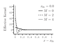
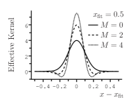
Figure 1: LOrPE effective kernel plots for a density that is sharply truncated at $0$, corresponding to support data points: (a) exactly at the boundary, (b) close to the boundary, and (c) away from the boundary.

3.2 Orthogonal series density estimation

The key idea underlying OSDE for a univariate density can be traced back to at least Čencov (1962). Updated monograph-length treatments of the topic can be found in Tarter & Lock (1993) and Efromovich (1999). There is a strong connection between LOrPE and OSDE. If $\{\phi_{k}\}$ is an orthonormal basis and $f$ is square integrable, then the classical OSDE of $f(x)$ is

$$\hat{f}_{\text{OSDE}}(x)=\sum_{j=0}^{J}\theta_{j}\phi_{j}(x),\qquad\text{where}\qquad\theta_{j}=\frac{1}{n}\sum_{i=1}^{n}\phi_{j}(x_{i}).$$ (13)

The tuning parameters here consist of the choice of basis functions and their number, $J$, to carry in the summation. In a more general form, and adapted for densities supported on $[a,b]$, this estimator can be represented as

$$\hat{f}_{\text{OSDE}}(x)=\frac{1}{b-a}+\sum_{j=1}^{\infty}w_{j}\theta_{j}\phi_{j}(x),$$ (14)

where the $w_{j}\in[0,1]$ are shrinkage coefficients (Efromovich, 1999). Comparing (9) and (14), we see immediately that LOrPE can be viewed heuristically as a localized version of OSDE, since the “basis functions” $\{P_{k}\}$ in the former are not global, but adjust locally depending on $x_{\mbox{\scriptsize\,fit}}$. Another facet of the connection between these estimators is revealed in the following theorem, which establishes that, for large bandwidths, LOrPE is essentially equivalent to OSDE with a Legendre polynomial basis.

Theorem 2

In the limit as $h\rightarrow\infty$, the LOrPE estimate (4) for pdf $f(x)$ with finite support $[a,b]$, reduces to classical OSDE in terms of the basis functions

$$\phi_{j}(x)=\sqrt{\frac{2}{b-a}}L_{j}\left(\frac{2x-a-b}{b-a}\right),$$

where the $\{L_{j}\}$ are orthonormal Legendre polynomials on $[-1,1]$.

Proof.

See the appendix. ∎

3.3 Local likelihood density estimation

In spirit (but not mathematical detail) LOrPE is also very similar to LLDE; see Hjort & Jones (1996), and Loader (1996, 1999). As observed by Loader (1999, ch. 5), LLDE overcomes boundary bias by matching localized sample moments to population moments using the log-polynomial density approximation (polynomial approximations on the log scale). As was noted in section 2, LOrPE instead matches localized expectation values of orthogonal polynomials to their sample values using polynomial density approximations (polynomial approximations on the original scale). Although the LLDE approach may be theoretically superior, LOrPE enjoys the pragmatic advantages of computational speed and numerical stability, as it does not involve the solution of non-linear equations at every grid point.

4 Selection of Tuning Parameters

This section discusses strategies for selecting the two LOrPE tuning parameters, bandwidth ($h$) and polynomial degree ($M$). (In principle the taper function $t(\cdot)$ could also be tuned, but for simplicity we restrict our attention to simple truncation.) We emphasize this dependence on tuning parameters by writing

$$\tilde{f}_{\text{LOrPE}}(x)\equiv\tilde{f}_{\text{LOrPE}}(x|h,M),$$

and discuss first an adaptation of the AMISE-optimal plug-in method for KDE (Silverman’s Rule). Methods based on cross-validation are also proposed. The performance of these approaches will be examined in section 5.

4.1 The plug-in approach

Note that from Theorem 1, LOrPE can be viewed as being equivalent to KDE with a high-order kernel, $K_{\mbox{\scriptsize\,eff}}$. The optimal AMISE expression for KDE with kernel function $K_{\mbox{\scriptsize\,eff}}(\cdot)$ of order $r$, is known to be (e.g., Wand & Jones, 1995),

$$\text{AMISE}_{h_{\ast}}(r)=\frac{2r+1}{2r}\left[2r(r!)^{-2}R_{\mbox{\scriptsize\,K${}_{\mbox{\scriptsize\,eff}}$}}(r)^{2r}\mu_{\mbox{\scriptsize\,K${}_{\mbox{\scriptsize\,eff}}$}}(r)^{2}R_{f^{(r)}}(r)n^{-2r}\right]^{1/(2r+1)},$$ (15)

with corresponding optimal value of $h$,

$$h_{\ast}(r)=\left[\frac{(r!)^{2}R_{\mbox{\scriptsize\,K${}_{\mbox{\scriptsize\,eff}}$}}(r)}{2rn\mu_{\mbox{\scriptsize\,K${}_{\mbox{\scriptsize\,eff}}$}}(r)^{2}R_{f^{(r)}}(r)}\right]^{1/(2r+1)},$$ (16)

where $f^{(r)}$ denotes the $r$-th derivative of $f$, and

$$\mu_{\mbox{\scriptsize\,K${}_{\mbox{\scriptsize\,eff}}$}}(r)=\int x^{r}K_{\mbox{\scriptsize\,eff}}(x)dx,\qquad R_{\mbox{\scriptsize\,K${}_{\mbox{\scriptsize\,eff}}$}}(r)=\int K_{\mbox{\scriptsize\,eff}}(x)^{2}dx,\qquad R_{f^{(r)}}(r)=\int f^{(r)}(x)^{2}dx.$$

The unknown moments $\mu_{\mbox{\scriptsize\,K${}_{\mbox{\scriptsize\,eff}}$}}(r)$ and $R_{\mbox{\scriptsize\,K${}_{\mbox{\scriptsize\,eff}}$}}(r)$ can be computed once the underlying kernel $K(\cdot)$ is selected; e.g., for Gaussian kernels we have Hermite polynomials, for beta kernels Gegenbauer polynomials, etc. For sample sizes in the range $10^{2}\leq n\leq 10^{4}$, optimal values of $r$ are likely to be relatively low, and thus these moments can be tabulated across a few $r$ values with a symbolic mathematics computer package, and then included in the relevant programs.

The only real difficulty is estimation of $R_{f^{(r)}}(r)$, but as explained by Wand & Jones (1995), a simple transformation leads to the expression $R_{f^{(r)}}(r)=(-1)^{r}\psi_{2r}$, and thus it suffices to study estimation of functionals $\psi_{s}\equiv\mathbb{E}[f^{(s)}(X)]$, for $s$ even. For this Wand & Jones (1995) propose multi-stage direct plug-in algorithms, involving the iteration of a KDE-type estimator of $\psi_{r}$ with optimal bandwidth that depends on $\psi_{s}$, $s>r$. Starting with a rough estimate of $\psi_{s}$ at some stage, which can be based on the well-known value corresponding to a $N(\mu,\sigma^{2})$, this is iterated to arrive at some estimate $\hat{\psi}_{s}$. A naive estimate of $\psi_{2r}$ follows by using an estimate of $\sigma$ (e.g., sample standard deviation). Plugging the resulting estimate of $R_{f^{(r)}}(r)$ into (15) gives eventually,

$$\text{AMISE}_{h_{\ast}}(r)\approx\frac{2r+1}{4r\hat{\sigma}}\left[\frac{2r(2r!)}{(r!)^{3}\sqrt{\pi}}\,\mu_{\mbox{\scriptsize\,K${}_{\mbox{\scriptsize\,eff}}$}}(r)^{2}\,\left(\frac{R_{\mbox{\scriptsize\,K${}_{\mbox{\scriptsize\,eff}}$}}(r)}{n}\right)^{2r}\right]^{1/(2r+1)}.$$ (17)

Now minimize (17) in $r$ to get $\hat{r}$ (which by Theorem 1 immediately provides also an estimate of $M$). Finally, substitute $\hat{r}$ into (16) to obtain the estimates

$$\hat{h}_{AMISE}=2\hat{\sigma}\left[\frac{(\hat{r}!)^{3}\sqrt{\pi}}{2\hat{r}(2\hat{r}!)n}\,\frac{R_{\mbox{\scriptsize\,K${}_{\mbox{\scriptsize\,eff}}$}}(\hat{r})}{\mu_{\mbox{\scriptsize\,K${}_{\mbox{\scriptsize\,eff}}$}}(\hat{r})^{2}}\right]^{1/(2\hat{r}+1)},\qquad\text{and}\qquad\hat{M}_{AMISE}=\begin{cases}\hat{r}+1,&\hat{r}\text{ even},\\ \hat{r}+2,&\hat{r}\text{ odd}.\end{cases}$$ (18)

Of course, this can only serve as a rough estimate, the intent being to provide reasonable initial values for a more refined search. The fact that LOrPE naturally self-adjusts near the support end points, complicates the calculation of the boundary contribution into the AMISE, as well as the analysis of the bias introduced by the truncation of the reconstructed density when forced to be non-negative (with subsequent renormalization).

4.2 Cross-validation methods

Least squares cross-validation (LSCV) for estimation of a generic PDF $f$ considers the integrated squared error of the density estimate,

$$ISE=\int{\left[\hat{f}(x)-f(x)\right]^{2}dx}.$$ (19)

As proposed by Bowman (1984) and Hall (1983), this leads eventually to minimization of the LSCV criterion. Applied to LOrPE, this yields

$$LSCV(h,M)=\int{\tilde{f}_{\text{LOrPE}}(x|h,M)^{2}dx}-\frac{2}{n}\sum_{i=1}^{n}\tilde{f}_{\text{LOrPE}}^{(-i)}(x_{i}|h,M),$$ (20)

where

$$\tilde{f}_{\text{LOrPE}}^{(-i)}(x|h,M)=\frac{1}{(n-1)h}\sum_{k=0}^{M}\sum_{\begin{subarray}{c}j=1\\ j\neq i\end{subarray}}^{n}P_{k}\left(\frac{x_{j}-x_{\mbox{\scriptsize\,fit}}}{h}\right)K\left(\frac{x_{j}-x_{\mbox{\scriptsize\,fit}}}{h}\right)P_{k}\left(\frac{x-x_{\mbox{\scriptsize\,fit}}}{h}\right),$$

is the leave-one-out LOrPE density estimate from (4), obtained by omitting the $i$-th observation. As suggested in the literature (e.g., Sheather, 2004), the existence of multiple minima means that it is prudent to plot $LSCV(h,M)$ over a grid of $h$ and $M$ values. From an asymptotic perspective, the main drawback of this criterion is its slow rate of convergence.

A related simpler and intuitively appealing but less popular approach, is likelihood cross-validation (LCV), the essential idea dating back to at least Habbema et al. (1974) and Duin (1976); see for example Silverman (1986) or Givens & Hoeting (2013, ch. 10) for an updated discussion. This is based on taking the likelihood function of the leave-one-out density estimate above, leading to minimization of

$$LCV(h,M)=\prod_{i=1}^{n}\tilde{f}_{\text{LOrPE}}^{(-i)}(x_{i}|h,M).$$

Reasoning that the density values at each point are taken from slightly different distributions (and not from the same distribution as in a genuine likelihood), the term pseudo-LCV might perhaps be more suitable.

An obvious obstacle with implementation of this criterion is the situation when $\tilde{f}_{\text{LOrPE}}^{(-i)}(x_{i}|h,M)=0$ for some $i$. Its use is also problematic for densities with infinite support due to the strong influence exerted by fluctuations in the tails. To avoid these situations a regularization condition can be introduced, leading to the modified regularized LCV (RLCV) criterion,

$$RLCV(h,M)=\prod_{i=1}^{n}\max\left\{\tilde{f}_{\text{LOrPE}}^{(-i)}(x_{i}|h,M),\frac{\tilde{f}_{\text{LOrPE}}^{(+i)}(x_{i}|h,M)}{n^{\alpha}}\right\},$$ (21)

where $\alpha>0$ is the regularization parameter, and

$$\tilde{f}_{\text{LOrPE}}^{(+i)}(x|h,M)=\frac{1}{nh}\sum_{k=0}^{M}P_{k}\left(\frac{x_{i}-x_{\mbox{\scriptsize\,fit}}}{h}\right)K\left(\frac{x_{i}-x_{\mbox{\scriptsize\,fit}}}{h}\right)P_{k}\left(\frac{x-x_{\mbox{\scriptsize\,fit}}}{h}\right),$$

is the contribution of data point $x_{i}$ toward the LOrPE density estimate (4). Note therefore that for each $i=1,\ldots,n$ we have

$$\tilde{f}_{\text{LOrPE}}(x|h,M)=\tilde{f}_{\text{LOrPE}}^{(+i)}(x|h,M)+\frac{n-1}{n}\tilde{f}_{\text{LOrPE}}^{(-i)}(x|h,M).$$

The case for regularizing LCV was made as early as Schuster & Gregory (1981) who remarked that for tails exponential and heavier, the use of LCV without regularization results in inconsistent density estimates. From a large number of simulations, we have noted that $\alpha=0.5$ is a reasonable default value. Of course, one can also add $\alpha$ to the list of tuning parameters to be selected via RLCV, a possibility that will be explored in section 5.

4.3 Effective degrees of freedom and shrinkage

In situations where truncation of the density below zero is unnecessary, LOrPE functions as a linear smoother of the EDF, analogously to KDE. This can be seen by taking the definition of the KDE effective kernel from Theorem 1, and observing that we can write (4) as

$$\tilde{f}_{\text{LOrPE}}(x)=\int\frac{1}{h}K_{\mbox{\scriptsize\,eff}}\left(\frac{x-y}{h}\right)\hat{f}_{\text{EMP}}(y)dy.$$

This suggests the possibility of adapting the idea of effective degrees of freedom for linear smoothers in a regression setup (Buja et al., 1989), to the analogous situation of density estimation. If $S$ is the smoothing matrix, the first of three sensible definitions for the effective degrees of freedom in a linear smoother, as given by Buja et al. (1989), is $\text{tr}(SS^{T})$.

For an arbitrary bandwidth, calculation of this trace appears to be analytically intractable due to edge effects. However, in the limit as $h\rightarrow\infty$, recall from Theorem 2 that LOrPE converges to OSDE in terms of Legendre polynomials. Now, for a density fit by a polynomial of degree $M$, the number of degrees of freedom of the fit (number of free parameters) is obviously $M$ ($M+1$ coefficients minus the one constraint from normalizing the PDF). As the effective degrees of freedom in a smoother is not limited to integers, this motivates a natural extension of LOrPE to non-integer values of $M$. Through suitable choice of the taper function, we can ensure that the effective degrees of freedom in any given fit is always $M$.

To formalize this, consider without loss of generality a PDF supported on $[-1,1]$. With $t(\cdot)$ a chosen taper function and the $\{L_{k}\}$ defined as in Theorem 2, OSDE smoothing is then seen to be performed by the linear operator $S(x,y)=\sum_{k=0}^{\infty}t(k)L_{k}(x)L_{k}(y)$, in an appropriate inner product space. Requiring the inner product with the EDF to yield OSDE, motivates the following definition:

$$\hat{f}_{\text{OSDE}}(x)=\langle S(x,y),\hat{f}_{\text{EMP}}(y)\rangle\equiv\int_{-1}^{1}S(x,y)\hat{f}_{\text{EMP}}(y)dy=\frac{1}{n}\sum_{i=1}^{n}\sum_{k=0}^{\infty}t(k)L_{k}\left(x\right)L_{k}\left(x_{i}\right).$$

This is now in the form of (14), with the $t(k)$ playing the role of the shrinkage coefficients $w_{k}$. The operator $S$ is in fact self-adjoint (symmetric), so that

$$SS^{T} = \langle S(x,z),S(z,y)\rangle=\int_{-1}^{1}S(x,z)S(z,y)dz$$

$$= \int_{-1}^{1}\sum_{k=0}^{\infty}t(k)L_{k}(x)L_{k}(z)\sum_{j=0}^{\infty}t(j)L_{j}(z)L_{j}(y)dz$$

$$= \sum_{k=0}^{\infty}t^{2}(k)L_{k}(x)L_{k}(y),$$

the last line following from identity (24). Additionally, note that we have

$$\text{tr}(SS^{T})=\int_{-1}^{1}SS^{T}\delta(x-y)dxdy=\int_{-1}^{1}\sum_{k=0}^{\infty}t^{2}(k)L_{k}^{2}(x)dx=\sum_{k=0}^{\infty}t^{2}(k).$$

Adapting the above definition for the effective degrees of freedom from Buja et al. (1989) to density estimation, we therefore arrive at the identity

$$M=\text{tr}(SS^{T})-1=\sum_{k=0}^{\infty}t^{2}(k)-1.$$ (22)

There are many possible choices for $t(\cdot)$ which would make (22) work, but perhaps the simplest is to take the step function approach of section 2. However, if the optimal $M$ is not an integer, an extra adjustment is needed, so that a more general prescription (with $m=\lfloor M\rfloor$ denoting the largest integer less than or equal to $M$) is to define:

$$t(k)=\begin{cases}1,&k\leq m,\\ \sqrt{M-m},&k=m+1,\\ 0,&k\geq m+2.\end{cases}$$

Throughout the paper, we adopt these shrinkage coefficients in all instances where LOrPE is applied, for any given bandwidth $h$.

5 Simulations

The primary goal of this section is to compare the MISE performance of LOrPE with that of its main competitor, KDE. This will be done both from oracle and non-oracle based perspectives. The oracle based comparisons, so called because the optimization has access to the true analytical ISE, are aimed at benchmarking the performance of the two methods, especially with regard to estimating densities that are sharply truncated. The non-oracle based comparisons will explore the performance of LOrPE to all of its rivals and analogues discussed thus far: KDE, OSDE, and LLDE.

To produce a spanning set of densities $f$ to be investigated, some elements from the list in Wand & Jones (1995, Table 2.2) were employed as a starting point. This includes the KDE-optimal Beta(4,4) on $(-1,1)$, as derived by Terrell (1990) for minimizing AMISE through minimization of total curvature. To these were added a few that are sharply truncated. Table 1 lists the choice of distributions selected for the simulation study, where $\phi(z)$ and $\Phi(z)$ denote the PDF and CDF of a standard normal. In particular, there are three distributions with sharp boundaries: two standard normals, one truncated at $0$ and the other at $-1$, and a standard exponential. It is expected that KDE will handle the N(0,1) truncated at $0$ well using data reflection (or mirroring), and it would therefore be interesting to compare its performance with that of LOrPE which does not enjoy this advantage. On the other hand, we would expect to see LOrPE outperform KDE for the N(0,1) truncated at $-1$, as the data reflecting method doesn’t work well in this case (due to discontinuity of the first derivative).

Table 1: List of distributions for simulations.

Name of $X$	Distribution/Density of $X$
Beta(4,4) on $[-1,1]$	$f^{*}(x)=\frac{35}{32}(1-x^{2})^{3}I(|x|<1)$
(optimal by KDE)
N(0,1)	$f(x)=\phi(x)$
Normal Mix 1	$X\sim\frac{3}{4}Z_{1}+\frac{1}{4}Z_{2}$
(bimodal)	$Z_{1}\sim\text{N}(0,1)$ and $Z_{2}\sim\text{N}(3/2,1/9)$
Exponential(1)	$f(x)=e^{-x}I(x>0)$
(sharp boundary at $0$)
N(0,1) on $[0,\infty)$	$f(x)=2\phi(x)I(x>0)$
(truncated at $0$)
N(0,1) on $[-1,\infty)$	$f(x)=\frac{1}{\Phi(1)}\phi(x)I(x>-1)$
(truncated at $-1$)
Normal Mix 2	$X\sim\frac{2}{3}Z_{1}+\frac{1}{3}Z_{2}$
(sharp peak at $0$)	$Z_{1}\sim\text{N}(0,1)$ and $Z_{2}\sim\text{N}(0,1/100)$

5.1 Oracle MISE comparisons: LOrPE vs. KDE

The “oracle” MISE comparisons, called “best case” by Jones & Henderson (2007), are useful for benchmarking LOrPE vs. KDE in determining the best possible performance for each method with regard to estimation of a particular density. Dassanayake (2014) details the procedure used to effect these comparisons for each of the distributions in Table 1. This involves performing a computationally intensive search for the optimal $h^{\ast}$ and $M^{\ast}$ that minimize the MISE over grids of polynomial degree values, $M\in\mathcal{M}$, and bandwidths $h\in\mathcal{H}$. MISEs were calculated by averaging 1,000 numerical estimates of ISE values (19). For KDE, $M$ is related to the kernel order via result (iii) of Theorem 1, and is therefore the approximate kernel order.

Figure 2 displays the resulting $\log_{10}(\text{MISE}(h^{\ast},M))$ values as a function of $M$, for each of LOrPE and KDE, and sample sizes of $n=10^{3}$ and $n=10^{5}$.

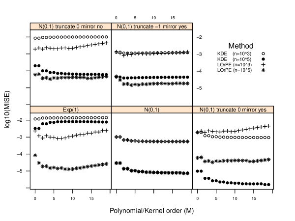
Figure 2: Oracle MISE values for sample sizes $n=10^{3}$ and $n=10^{5}$, as a function of polynomial order $M$ (LOrPE) or approximate kernel order $M$ (KDE).

According to these graphical summaries, it is clear that LOrPE works in a similar manner to KDE when estimating densities with exponentially declining tails at both ends of the support, such as the $N(0,1)$. Similar results were observed for the Beta$(4,4)$, and the two Normal Mixes (not shown). For densities with sharp edges, LOrPE tends to attain lower MISE values than KDE. The $N(0,1)$ truncated at $0$ (with KDE mirroring) is a notable exception; but the better performance of KDE is only really discernible at larger sample sizes and higher kernel orders. If the crucial data mirroring property of KDE at the boundaries is removed, then the tables are reversed in favor of LOrPE, particularly at small sample sizes and low kernel orders. The Exponential$(1)$ constitutes a dramatic case in favor of LOrPE, while the $N(0,1)$ truncated at $-1$ (with KDE benefiting from mirroring) is somewhere in between these two extremes. Note that LOrPE does not use data mirroring (although it can use kernel mirroring whereby the weight function is reflected at the boundary and added to the non-reflected part).

The appropriate minimum oracle $\log_{10}(\text{MISE}(h^{\ast},M^{\ast}))$ values for all the densities of Table 1, are displayed in Table 2, along with the corresponding optimal $(M^{\ast},h^{\ast})$. Note that all truncated $N(0,1)$ KDE values were obtained using data mirroring, whereas the un-truncated $N(0,1)$ did not. As can be seen, at lower sample sizes all LOrPE estimates have lower (or the same) MISE, except for the truncated normals. However, this KDE advantage for the truncated normal at $-1$ gradually erodes, so that at higher sample sizes only the KDE estimates for the $0$ truncated $N(0,1)$ persist in having lower MISE than LOrPE.

Table 2: Oracle $log_{10}(\text{MISE})$ values for the densities in Table 1 as a function of sample size. The values in parentheses correspond to the optimal $(M^{\ast},h^{\ast})$, where $M$ is the polynomial order (LOrPE) or approximate kernel order (KDE) and $h$ is the bandwidth. For each density and each $n$, the lowest of the two MISE values appears in bold face.

	$n=10^{2}$		$n=10^{3}$		$n=10^{4}$
Distribution	LOrPE	KDE	LOrPE	KDE	LOrPE	KDE
N(0,1)	-2.441	-2.440	-3.260	-3.260	-4.177	-4.177
	(19, 11.4)	(13, 8.3)	(16, 8.2)	(17, 8.2)	(17, 7.0)	(17, 7.0)
Normal Mix 1	-2.014	-2.014	-2.774	-2.774	-3.661	-3.661
	(0, 1.0)	(0, 1.0)	(4, 1.5)	(4, 1.5)	(11, 2.0)	(11, 2.0)
Normal Mix 2	-1.378	-1.370	-2.208	-2.208	-3.108	-3.108
	(0, 0.25)	(2, 0.43)	(6, 0.51)	(6, 0.51)	(14, 0.74)	(14, 0.74)
N(0,1) on $[0,\infty)$	-2.243	-2.475	-2.997	-3.318	-3.869	-4.213
	(0, 1.2)	(17, 9.7)	(2, 1.9)	(19, 8.6)	(4, 2.7)	(18, 7.5)
N(0,1) on $[-1,\infty)$	-2.223	-2.241	-3.091	-2.609	-3.932	-3.010
	(2, 3.0)	(4, 3.9)	(2, 2.1)	(1, 0.79)	(2, 1.6)	(0, 0.19)
Beta(4,4)	-2.044	-2.064	-2.890	-2.886	-3.824	-3.705
	(4, 13.0)	(8, 2.04)	(4, 1.5)	(10, 2.9)	(6, 11.6)	(9, 1.5)
Exponential(1)	-2.265	-1.462	-3.085	-1.954	-4.002	-2.392
	(2, 4.1)	(0, 0.48)	(6, 13.2)	(0, 0.16)	(8, 13.7)	(0, 0.082)

5.2 Non-oracle MISE comparisons

The intent in this section is to compare LOrPE MISE values to those of its closest competitors, KDE, LLDE, and OSDE, in a realistic (non-oracle) setting. In order to make these comparisons as fair as possible in terms of mimicking an unsophisticated user, “reasonable” default settings were used for the the respective tuning parameters of each method. The details are as follows.

LOrPE:

Uses the plug-in estimates from (18), implemented via the NPStat package (Volobouev, 2012).

KDE:

Uses the Sheather & Jones (1991) two-stage plug-in (”dpi” or ”direct plug-in”) bandwidth with a normal kernel and sample standard deviation as the estimate of scale, implemented via R library ks.

LLDE:

Uses the above KDE plug-in bandwidth, a Gaussian kernel, and zero-order polynomial, implemented via the R library locfit.

OSDE:

The estimator in (13) was coded with the number of terms, $J$, chosen according to the Hart (1985) scheme. The NPStat package (Volobouev, 2012) is used to generate the necessary orthogonal polynomials on a grid (consisting of 2,048 points). The lowest and highest order statistics from the sample of size $n$ are mapped to the $1/(2n)$ and $1-1/(2n)$ quantiles, respectively. All other points are then mapped linearly using these two extremes. The support of the density is now estimated by inversely mapping the $[0,1]$ interval. The discrete analog of Legendre polynomials are employed; generated by the Gram-Schmidt procedure for a uniform weight on the grid in $[0,1]$.

MISEs were calculated empirically as in section 5.1. The data were once again simulated from most of the distributions in Table 1, as well as Student’s $t$ with 1, 2, and 3 degrees of freedom truncated to the interval $[-1,2]$. The results are presented on Table 3 which summarizes the $log_{10}(\text{MISE})$ values for three different sample sizes within each distribution. We note that LOrPE yields consistently minimum MISE values for the sharply truncated normal distributions and the Exponential. For the truncated $t$ distributions the results are mixed, but LOrPE tends to dominate for larger sample sizes. In nearly all cases where LOrPE does not yield the minimum MISE, it is a close second.

Table 3: Non-oracle $log_{10}(\text{MISE})$ values for 4 estimators of the true density. MISEs are based on 1,000 realizations simulated from a variety of distributions and sample sizes ($n$). For each distribution and each $n$, the lowest of the 4 MISE values appears in bold face.

Distribution	$log_{10}(n)$	LOrPE	KDE	LLDE	OSDE
N(0,1)	$2$	-2.138	-2.198	-2.183	-1.634
	$3$	-3.088	-2.973	-3.179	-1.650
	$4$	-4.045	-3.741	-4.158	-2.652
N(0,1) on $[0,\infty)$	$2$	-2.177	-1.576	-1.427	-1.666
	$3$	-2.923	-2.010	-1.594	-2.642
	$4$	-3.770	-2.392	-1.613	-3.634
N(0,1) on $[-1,\infty)$	$2$	-2.085	-2.023	-1.837	-1.823
	$3$	-3.005	-2.564	-2.188	-2.799
	$4$	-3.874	-2.980	-2.248	-3.776
Normal Mix 1	$2$	-1.743	-1.888	-1.824	-1.148
	$3$	-2.108	-2.223	-2.028	-1.149
	$4$	-2.477	-2.278	-2.060	-1.149
Exponential(1)	$2$	-2.239	-1.374	-1.299	-0.677
	$3$	-2.915	-1.783	-1.386	-1.2328
	$4$	-3.740	-2.157	-1.393	-0.679
$t(1)$ on $[-1,2]$	$2$	-1.891	-2.317	-2.447	-1.347
	$3$	-2.712	-2.694	-3.000	-2.337
	$4$	-3.661	-3.118	-3.128	-3.337
$t(2)$ on $[-1,2]$	$2$	-1.980	-2.346	-2.366	-1.408
	$3$	-2.839	-3.065	-3.191	-2.404
	$4$	-3.724	-3.546	-3.591	-3.400
$t(3)$ on $[-1,2]$	$2$	-2.039	-2.328	-2.289	-1.437
	$3$	-2.879	-3.061	-3.207	-2.427
	$4$	-3.769	-3.856	-3.763	-3.416

5.3 Oracle and non-oracle MISE comparisons: LOrPE vs. KDE

Recall that the LOrPE plug-in approach is meant to serve as an initial estimate in a more refined search for appropriate $h$ and $M$ values. Since plug-in formulae do not take boundary effects into account, we would expect sub-optimal performance from LOrPE in regard to estimation in the vicinity of the support boundary. The already good LOrPE plug-in performance seen in section 5.2 could therefore potentially be improved by using cross-validation methods. Given that oracle comparisons provide lower bounds on MISE values, we may ask two interesting questions of LOrPE cross-validation methods: (i) how close can they get to LOrPE oracle values, and (ii) how close can they get to KDE oracle values.

This section aims to answer these questions, using both the LSCV and RLCV criteria, as described by equations (20) and (21), respectively, with the regularization parameter set at $\alpha=0.5$ in the latter. Both oracle and non-oracle methods are considered, and as such the simulation details for the former parallel those of section 5.1, while those for the latter are identical to section 5.2. For KDE oracle computations: the $N(0,1)$ and $N(0,1)$ truncated at $-1$ did not use data mirroring, while the $N(0,1)$ truncated at $0$ used mirroring. This time a variety of sample sizes were considered in order to reveal any possible convergence of methods as $n\rightarrow\infty$. Also, for brevity only 6 of the (representative) distributions listed in Table 3 were examined.

The resulting $log_{10}(\text{MISE})$ values appear plotted vs. sample size in Figure 3. The answer to the above two questions seems clear. First, LOrPE cross-validation methods come very close to LOrPE oracle values, with the RLCV criterion dominating LSCV most of the time. Secondly, and remarkably, except for the $N(0,1)$ and $0$ truncated $N(0,1)$, LOrPE cross-validation methods produce consistently lower MISE values than KDE oracle.

Figure 3: Plots of oracle (solid lines) and non-oracle $log_{10}(\text{MISE})$ values for LOrPE and KDE. The non-oracle methods of LSCV (dashed lines) and RLCV (dotted lines) apply only to LOrPE.

In some cases, and especially at small sample sizes, the LOrPE-RLCV method may not be achieving the lowest possible MISE. One reason for this could be that the regularization parameter choice of $\alpha=0.5$ is not optimal. To investigate this issue, Figure 4 plots the $log_{10}(\text{MISE})$ values vs. $\alpha\in[0,1]$ for the distributions considered in Figure 3, and for sample size $n=10^{3}$ only. The error bars around each value extend from the $84.13^{th}$ to the $15.87^{th}$ percentiles divided by $2\sqrt{n}$, and provide a sense of sampling variability through a robust measure of the standard error. It is clear that, perhaps with the exception of the $N(0,1)$ case, LOrPE-RLCV is reasonably insensitive to the choice of $\alpha$. This suggests that it may not be necessary to estimate this extra tuning parameter, and just use a default value of $\alpha=0.5$.

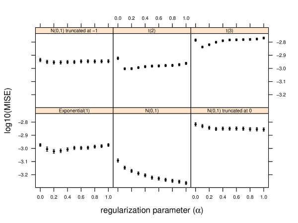
Figure 4: Plots of $log_{10}(\text{MISE})$ values vs. the regularization parameter $\alpha$ for the LOrPE-RLCV method applied to 1,000 simulated datasets of sample size $n=10^{3}$. The error bars provide a robust measure of the standard error.

6 Real Data Application

As an illustration of the proposed methodology, we consider the lengths of $n=86$ spells of psychiatric treatment (days) undergone by patients used as controls in a study of suicide risks (Copas & Fryer, 1980). The data were presented by Silverman (1986, Table 2.1), who used them to demonstrate certain inadequacies with KDE. Scaled to the unit interval by dividing all observations by the largest value of 737, it is publicly available in the R library bde as ”suicide.r”. Figure 5 displays a histogram with rugplot, and five density estimates. Sturges’ formula is used to compute the breaks and number of classes in the histogram shaded in gray (the default in R function “hist”).

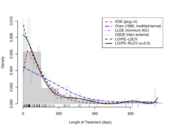
Figure 5: Density estimates for the Suicide data: KDE (red/dashed), Chen (1999) (blue/longdash), LLDE (purple/dotdash), OSDE (green/dotted), LOrPE-LSCV (black/dashed), LOrPE-RLCV (black/solid).

KDE (red dashed lines) uses the plug-in bandwidth as described in section 5.2. As expected, there is an apparent bias at the left end of the support, the estimate dips down toward zero, whereas the data suggests there should be a large amount of mass in that vicinity. A similar outcome occurs with LLDE (purple dotdash lines), which displays less “wigglyness” in the tail, but a sharp “kink” at the peak. As suggested by Loader (1999), greater care was exercised in selecting appropriate values for the LLDE tuning parameters: we used AIC to identify the optimal nearest neighbor component of the smoothing parameter and polynomial order, instead of the (quicker) KDE plug-in bandwidth and degree zero of section 5.2, as a means of specifying the effective degrees of freedom. No appreciable changes were observed with kernels different from Gaussian. OSDE (green dotted lines) obviously undersmoothes badly, a consequence of the degree preferred by Hart’s (1985) method being $J=48$.

Rather more believable performance was obtained with Chen’s (1999) boundary-corrected beta-kernel density estimator (blue longdash lines), which picks up the mass at the peak, but seems to be somewhat oversmoothed. This is Chen’s (1999) second beta-kernel estimator, called “modified” in the R library bde with which it is implemented, since Chen (1999) showed it consistently outperforms the first beta-kernel estimator. The critical bandwidth tuning parameter is set at the default value of $b=n^{-2/5}$, the AMISE optimal order for such kernels (Chen, 1999). Finally, we note the arguably superior performance of LOrPE (black dashed and solid lines). LORPE-RLCV uses the default value of $\alpha=0.5$ for the regularization parameter, as suggested by the simulations in section 5.3, and the optimal degree and bandwidth were $M=7$ and $h=2047.2$. LORPE-LSCV delivers a similar performance with $M=2.9$ and $h=605.3$.

7 Summary Remarks

We have shown that LOrPE is a useful extension to the (already vast) array of tools for nonparametric density estimation. This novel idea has at its basis the local expansion of the EDF into a series of orthogonal polynomials around a selection of grid points. It was demonstrated that away from the support boundary LOrPE essentially functions like KDE with a high-order kernel, whereas close to the boundary LOrPE is adaptive in the sense that its effective kernels naturally change shape to accommodate the endpoint, thereby reducing boundary bias. Faster asymptotic convergence rates follow naturally by virtue of the higher-order kernels. LOrPE also shares important connections with LLDE and OSDE. Simulations demonstrated that LOrPE generally outperforms these estimators, and especially KDE, when estimating densities with sharp boundaries. Also, LOrPE allows for the inclusion of a taper function, a feature which takes LOrPE beyond KDE with high-order kernels.

These reasons make LOrPE applicable in a wider range of problems than KDE. When estimating distributions which decay rapidly at infinity, LOrPE results are identical to KDE. Additionally, the local polynomial modeling can effectively reduce the bias for densities with several (at least $M$) continuous derivatives. A proper balance of $h$ and $M$ can thus result in a better overall estimator. Cross-validation, and especially a regularized version of likelihood cross-validation, seems to be a promising way of selecting appropriate values for these tuning parameters. For large $n$, the simulations suggest LOrPE MISE approaches the oracle (or “best case”) MISE. Finally, LOrPE calculations remain essentially unchanged in multivariate settings, requiring only a switch to multivariate orthogonal polynomial systems.

Appendix A Proof of Theorem 1

Substituting the expression for $c_{k}(\cdot)$ from (8) into (9) gives

$$\tilde{f}_{\text{LOrPE}}(x) = \sum_{k=0}^{\infty}t(k)c_{k}(x_{\mbox{\scriptsize\,fit}},h)P_{k}\left(\frac{x-x_{\mbox{\scriptsize\,fit}}}{h}\right)$$

$$= \sum_{k=0}^{\infty}t(k)\left\{\frac{1}{nh}\sum_{i=1}^{n}P_{k}\left(\frac{x_{i}-x_{\mbox{\scriptsize\,fit}}}{h}\right)K\left(\frac{x_{i}-x_{\mbox{\scriptsize\,fit}}}{h}\right)\right\}P_{k}\left(\frac{x-x_{\mbox{\scriptsize\,fit}}}{h}\right)$$

$$= \frac{1}{nh}\sum_{i=1}^{n}\underbrace{\left\{\sum_{k=0}^{\infty}t(k)P_{k}\left(\frac{x-x_{\mbox{\scriptsize\,fit}}}{h}\right)P_{k}\left(\frac{x_{i}-x_{\mbox{\scriptsize\,fit}}}{h}\right)K\left(\frac{x_{i}-x_{\mbox{\scriptsize\,fit}}}{h}\right)\right\}}_{K_{\mbox{\scriptsize\,eff}}\left(\frac{x-x_{i}}{h}\right)}$$

$$= \frac{1}{nh}\sum_{i=1}^{n}K_{\mbox{\scriptsize\,eff}}\left(\frac{x-x_{i}}{h}\right)$$

Defining $y=(x_{\mbox{\scriptsize\,fit}}-x_{i})/h$, evaluate $K_{\mbox{\scriptsize\,eff}}$ at grid point $x_{\mbox{\scriptsize\,fit}}$ to see that

$$K_{\mbox{\scriptsize\,eff}}\left(\frac{x_{\mbox{\scriptsize\,fit}}-x_{i}}{h}\right)\equiv K_{\mbox{\scriptsize\,eff}}\left(y\right)=\sum_{k=0}^{\infty}t(k)P_{k}\left(0\right)P_{k}\left(-y\right)K\left(-y\right).$$

To establish (i)–(iii), note that Assumptions (a) and (b) imply that $P_{k}(x)$ is an even (odd) function for any even (odd) integer $k$. This means $P_{k}(-x)=P_{k}(x)$ for $k$ even, and $P_{k}(0)=0$ for $k$ odd, so that the effective kernel becomes

$$K_{\mbox{\scriptsize\,eff}}\left(x\right)=\sum_{\{k\,:\,k\geq 0,\ k\text{ even}\}}t(k)P_{k}\left(0\right)P_{k}\left(x\right)K\left(x\right),$$ (23)

and $K_{\mbox{\scriptsize\,eff}}(-x)=K_{\mbox{\scriptsize\,eff}}(x)$ is an even function supported also on $(-a_{K},a_{K})$, thus establishing (i). Now, multiplying both sides of the above equation by $P_{0}(x)\equiv 1$ and integrating, gives

$$\int_{\mathbb{R}}K_{\mbox{\scriptsize\,eff}}(x)dx = \int_{-a_{K}}^{a_{K}}K_{\mbox{\scriptsize\,eff}}(x)P_{0}(x)dx$$

$$= \int_{\tilde{a}_{\mbox{\scriptsize\,fit}}}^{\tilde{b}_{\mbox{\scriptsize\,fit}}}\sum_{\{k\,:\,k\geq 0,\ k\text{ even}\}}t(k)P_{k}(0)P_{0}(x)P_{k}(x)K(x)dx,$$

which follows by Assumption (c). Now, interchanging integral and sum in the above expression and then using (6), establishes (ii) as follows:

$$\int_{\mathbb{R}}K_{\mbox{\scriptsize\,eff}}(x)dx = \sum_{\{k\,:\,k\geq 0,\ k\text{ even}\}}t(k)P_{k}(0)\int_{\tilde{a}_{\mbox{\scriptsize\,fit}}}^{\tilde{b}_{\mbox{\scriptsize\,fit}}}P_{0}(x)P_{k}(x)K(x)dx$$

$$= \sum_{\{k\,:\,k\geq 0,\ k\text{ even}\}}t(k)P_{k}(0)\delta_{0\,k}$$

$$= t(0)P_{0}(0)=t(0).$$

To prove (iii), first define the $j$-th kernel moment as

$$\mu_{j}(K_{\mbox{\scriptsize\,eff}})\equiv\int_{\mathbb{R}}x^{j}K_{\mbox{\scriptsize\,eff}}(x)dx.$$

Now, since the effective kernel is an even function, it is clear $\mu_{j}(K_{\mbox{\scriptsize\,eff}})=0$ for $j$ odd. Hence, it suffices to consider the case when $j$ is even, whence

$$\mu_{j}(K_{\mbox{\scriptsize\,eff}})=\int_{\mathbb{R}}x^{j}K_{\mbox{\scriptsize\,eff}}(x)dx=\sum_{\{k\,:\,0\leq k\leq M,\ k\text{ even}\}}P_{k}(0)\int_{-a_{K}}^{a_{K}}x^{j}P_{k}(x)K(x)dx=\sum_{\{k\,:\,0\leq k\leq M,\ k\text{ even}\}}\alpha_{jk}P_{k}(0),$$

if we define

$$\alpha_{jk}=\int_{-a_{K}}^{a_{K}}x^{j}P_{k}(x)K(x)dx=\int_{\tilde{a}_{\mbox{\scriptsize\,fit}}}^{\tilde{b}_{\mbox{\scriptsize\,fit}}}x^{j}P_{k}(x)K(x)dx.$$

Now, from the theory of orthogonal polynomials, we know that

$$x^{j}=\sum_{k=0}^{j}a_{jk}P_{k}(x),\qquad\text{where}\qquad a_{jk}=\int_{\tilde{a}_{\mbox{\scriptsize\,fit}}}^{\tilde{b}_{\mbox{\scriptsize\,fit}}}x^{j}P_{k}(x)K(x)dx=\alpha_{jk}.$$

Since $\alpha_{jk}$ is the coefficient of the $P_{k}(x)$ contribution (a polynomial of order $k$) to the series expansion of $x^{j}$, it is obvious that $\alpha_{jk}=0$ for $k>j$, and $\alpha_{jk}=0$ when $k$ and $j$ have opposite parity (only even $k$ terms contribute when $j$ is even, and vice-versa). With these observations, it is clear that for $j\leq M$

$$\mu_{j}(K_{\mbox{\scriptsize\,eff}})=\sum_{k=0}^{M}\alpha_{jk}P_{k}(0),\qquad\text{and}\qquad x^{j}=\sum_{k=0}^{M}\alpha_{jk}P_{k}(x),$$

whence we see that

$$\mu_{j}(K_{\mbox{\scriptsize\,eff}}) = \left.x^{j}\right|_{x=0}=\begin{cases}1,&j=0,\\ 0,&j=1,\ldots,M.\end{cases}$$

If $M$ is even, then since $M+1$ is odd and $K_{\mbox{\scriptsize\,eff}}(x)$ is an even function, we have additionally that $\mu_{M+1}(K_{\mbox{\scriptsize\,eff}})=0$. Thus the effective kernel order is $M+1$ if $M$ is odd, and $M+2$ if $M$ is even.

Appendix B Proof of Theorem 2

As $h\rightarrow\infty$ the value of the kernel $K(\cdot)$ becomes less and less dependent on the grid point $x_{\mbox{\scriptsize\,fit}}$ inside $[a,b]$. In fact, starting from (5), note that for very large h, $K((x_{i}-x_{\mbox{\scriptsize\,fit}})/h)$ essentially becomes constant on $[a,b]$. Equation (4) then gives rise to Legendre polynomials since these are generated when integrating with respect to a constant weight function, in a manner similar to Proposition 1. To see this, start with the orthonormal Legendre polynomials $L_{k}(z)$ on $[-1,1]$, satisfying

$$\delta_{jk}=\int_{-1}^{1}L_{j}(z)L_{k}(z)dz.$$ (24)

To construct the corresponding orthonormal system on $[a,b]$, we make the transformation, $z=(2x-a-b)/(b-a)$, so that (24) becomes

$$\delta_{jk} = \int_{a}^{b}\frac{2}{b-a}L_{j}\left(\frac{2x-a-b}{b-a}\right)L_{k}\left(\frac{2x-a-b}{b-a}\right)dx=\int_{a}^{b}P_{j}\left(x\right)P_{k}\left(x\right)dx,$$ (25)

where

$$P_{k}(x)\equiv\sqrt{\frac{2}{b-a}}L_{k}\left(\frac{2x-a-b}{b-a}\right).$$ (26)

Now construct an orthonormal system on the interval $[\tilde{a}_{\mbox{\scriptsize\,fit}},\tilde{b}_{\mbox{\scriptsize\,fit}}]$ using $K(0)$ as the weight function instead of 1. By means of the transformation $y=(x-x_{\mbox{\scriptsize\,fit}})/h$, (25) then becomes

$$\delta_{jk} = \int_{a}^{b}\frac{1}{\sqrt{K(0)}}P_{j}\left(x\right)\frac{1}{\sqrt{K(0)}}P_{k}\left(x\right)K(0)dx$$

$$= \int_{\tilde{a}_{\mbox{\scriptsize\,fit}}}^{\tilde{b}_{\mbox{\scriptsize\,fit}}}\sqrt{\frac{h}{K(0)}}P_{j}\left(yh+x_{\mbox{\scriptsize\,fit}}\right)\sqrt{\frac{h}{K(0)}}P_{k}\left(yh+x_{\mbox{\scriptsize\,fit}}\right)K(0)dy$$

$$= \int_{\tilde{a}_{\mbox{\scriptsize\,fit}}}^{\tilde{b}_{\mbox{\scriptsize\,fit}}}\tilde{P}_{j}(y)\tilde{P}_{k}(y)K(0)dy$$

where

$$\tilde{P}_{k}(y)\equiv\sqrt{\frac{2h}{(b-a)K(0)}}L_{k}\left(\frac{2yh+2x_{\mbox{\scriptsize\,fit}}-a-b}{b-a}\right),$$ (27)

which follows from (26). Now, from the proof of Theorem 1 we have the following expression for LOrPE:

$$\tilde{f}_{\text{LOrPE}}(x)=\frac{1}{nh}\sum_{i=1}^{n}\sum_{k=0}^{M}P_{k}\left(\frac{x-x_{\mbox{\scriptsize\,fit}}}{h}\right)P_{k}\left(\frac{x_{i}-x_{\mbox{\scriptsize\,fit}}}{h}\right)K\left(\frac{x_{i}-x_{\mbox{\scriptsize\,fit}}}{h}\right).$$

Substituting $\tilde{P}_{k}(\cdot)$ for $P_{k}(\cdot)$ in the above equation, gives

$$\tilde{f}_{\text{LOrPE}}(x) = \frac{1}{nh}\sum_{i=1}^{n}\sum_{k=0}^{M}\tilde{P}_{k}\left(\frac{x-x_{\mbox{\scriptsize\,fit}}}{h}\right)\tilde{P}_{k}\left(\frac{x_{i}-x_{\mbox{\scriptsize\,fit}}}{h}\right)K\left(\frac{x_{i}-x_{\mbox{\scriptsize\,fit}}}{h}\right)$$ (28)

$$= \frac{1}{nh}\sum_{i=1}^{n}\sum_{k=0}^{M}\frac{2h}{(b-a)K(0)}L_{k}\left(\frac{2\left(\frac{x-x_{\mbox{\scriptsize\,fit}}}{h}\right)h+2x_{\mbox{\scriptsize\,fit}}-a-b}{b-a}\right)$$ (30)

$$\qquad\qquad L_{k}\left(\frac{2\left(\frac{x_{i}-x_{\mbox{\scriptsize\,fit}}}{h}\right)h+2x_{\mbox{\scriptsize\,fit}}-a-b}{b-a}\right)K\left(\frac{x_{i}-x_{\mbox{\scriptsize\,fit}}}{h}\right)$$

$$= \frac{1}{n}\sum_{i=1}^{n}\sum_{k=0}^{M}\frac{2}{(b-a)K(0)}L_{k}\left(\frac{2x-a-b}{b-a}\right)L_{k}\left(\frac{2x_{i}-a-b}{b-a}\right)K\left(\frac{x_{i}-x_{\mbox{\scriptsize\,fit}}}{h}\right).$$ (31)

Since

$$\lim_{h\rightarrow\infty}K\left(\frac{x_{i}-x_{\mbox{\scriptsize\,fit}}}{h}\right)=K(0),$$

we obtain

$$\tilde{f}_{\text{LOrPE}}(x)=\frac{1}{n}\sum_{i=1}^{n}\sum_{k=0}^{M}\sqrt{\frac{2}{b-a}}L_{k}\left(\frac{2x-a-b}{b-a}\right)\sqrt{\frac{2}{b-a}}L_{k}\left(\frac{2x_{i}-a-b}{b-a}\right),$$ (32)

which is the classical OSDE (13) in terms of the orthogonal polynomials

$$\phi_{k}(x)=\sqrt{\frac{2}{b-a}}L_{k}\left(\frac{2x-a-b}{b-a}\right).$$

References

- [1] Bowman, A.W. (1984), “An alternative method of cross-validation for the smoothing of density estimates”, Biometrika, 71, 353–360.
- [2] Buja, A., Hastie, T., and Tibshirani, R. (1989), “Linear Smoothers and Additive Models”, The Annals of Statistics (with discussion), 17, 453–555.
- [3] Čencov, N.N. (1962), “Evaluation of an unknown distribution density from observations”, Soviet Math. Dokl., 3, 1559–1562.
- [4] Charpentier, A., Fermanian J.-D. and Scaillet, O. (2006), “The Estimation of Copulas: Theory and Practice” in: Rank, J. (ed.), Copulas: From Theory to Application in Finance, 35-60, Risk Books: London.
- [5] Chen, S.X. (1999), “Beta kernel estimators for density functions”, Comp. Statist Data Anal., 31, 131–45.
- [6] Chen, S.X. and Huang, T.M. (2007), “Nonparametric estimation of copula functions for dependence modelling”, Canadian Journal of Statistics, 35, 265-282.
- [7] Chiu, S.-T. (1992), “An Automatic Bandwidth Selector for Kernel Density Estimation”, Biometrika, 79, 771-782.
- [8] Copas, J.B. and Fryer, M.J. (1980), “Density Estimation and Suicide Risks in Psychiatric Treatment”, Journal of the Royal Statistical Society, Series A, 143, 167–176.
- [9] Dassanayake, D.P.A. (2014), Local Orthogonal Polynomial Expansion and Empirical Sadddlepoint Approximation for Density Estimation, PhD Dissertation, Texas Tech University, Lubbock.
- [10] Diggle, P.J. and Hall, P. (1986), “The selection of terms in an orthogonal series density estimator”, J. Americ. Statist. Assoc. 81, 230-233.
- [11] Duin, R.P.W. (1976), “On the choice of smoothing parameter for Parzen estimators of probability density functions” IEEE Trans. Computers, C-25, 1175–1179.
- [12] Efromovich, S. (1999), Nonparametric Curve Estimation: methods, theory, and applications, New York: Springer.
- [13] Elderton, W.P. and Johnson, N.L. (1969), Systems of Frequency Curves, New York: Cambridge University Press.
- [14] Gijbels, I. and Mielniczuk, J. (1990), “Estimating the Density of a Copula Function”, Communications in Statistics: Theory and Methods, 19, 445-464.
- [15] Givens, G.H. and Hoeting, J.A. (2013), Computational Statistics, 2nd ed., Hoboken: Wiley.
- [16] Habbema, J.D.F., Hermans, J. and van der Broek, K. (1974), ”A stepwise discrimination program using density estimation”, in Bruckman, G. (ed.), Compstat 1974, Vienna: Physica Verlag, 100–110.
- [17] Hall, P. and Marron, J.S. (1988), “Choice of kernel order in density estimation”, The Annals of Statistics, 16, 161-173.
- [18] Hall, P. and Tao, T. (2002), “Relative efficiencies of kernel and local likelihood density estimators”, Journal of the Royal Statistical Society, Series B, 64, 537-547.
- [19] Hall, P. (1983), “Large sample optimality of least squares cross-validation in density estimation”, Ann. Statist., 11, 1156–1174.
- [20] Hart, J.D. (1985), “On the choice of a truncation point in Fourier series density estimation”, J. Statist. Comput. Simulation, 21, 95–-116.
- [21] Heidenreich, N.-B., Schindler, A. and Sperlich, S. (2013), “Bandwidth selection for kernel density estimation: a review of fully automatic selectors”, Advances in Statistical Analysis 97, 403-433.
- [22] Hjort, N.L. and Jones, M.C. (1996), “Locally parametric nonparametric density estimation”, The Annals of Statistics, 24, 1619-1647.
- [23] Jones, M.C. and Henderson, D.A. (2007), “Kernel-type density estimation on the unit interval”, Biometrika, 94, 977–984.
- [24] Kakizawa, Y. (2004), “Bernstein polynomial probability density estimation”, J. Nonparametr. Stat., 16, 709–-729.
- [25] Loader, C.R. (1996), “Local Likelihood Density Estimation”, Ann. Statist. 24, 1602-1618.
- [26] Loader, C.R. (1999), Local Regression and Likelihood, New York: Springer.
- [27] Malec, P. and Schienle, M. (2014), “Nonparametric kernel density estimation near the boundary”, Computational Statistics and Data Analysis, 72, 57–76.
- [28] Schuster, E.F. and Gregory, C.G. (1981), ”On the inconsistency of maximum likelihood nonparametric density estimators”, in Eddy, W.F. (ed.), Computer Science and Statistics: Proceedings of the 13th Symposium on the Interface, New York: Springer-Verlag, 295–298.
- [29] Sheather, S.J. (2004), “Density Estimation”, Statist. Sci. 19, 588-597.
- [30] Sheather, S.J. and Jones, M.C. (1991), “A reliable data-based bandwidth selection method for kernel density estimation”, Journal of the Royal Statistical Society, series B, 53, 683-–690.
- [31] Scott, D.W. (1992), Multivariate Density Estimation: Theory Practice and Visualization, New York: Wiley.
- [32] Silverman, B.W. (1986), Density Estimation for Statistics and Data Analysis, London: Chapman & Hall.
- [33] Tarter, M.E. and Lock, M. (1993), Model-free Curve Estimation, New York: Chapman & Hall.
- [34] Terrell, G.R. (1990), “The maximal smoothing principle in density estimation”, J. Amer. Statist. Assoc., 85, 470–-477.
- [35] Thas, O. (2010), Comparing Distributions, New York: Springer.
- [36] Volobouev, I. (2011), “Matrix Element Method in HEP: Transfer Functions, Efficiencies, and Likelihood Normalization”, arXiv:1101.2259 [physics.data-an].
- [37] Volobouev, I. (2012), NPStat (Non-parametric Statistical Modeling and Analysis); software available at http://npstat.hepforge.org http://npstat.hepforge.org.
- [38] Wand, M. and Jones, M. (1995), Kernel Smoothing, London: Chapman & Hall.
- [39] Wasserman, L. (2006), All of Nonparametric Statistics, New York: Springer.
- [40] Wigmans, R. (2000), Calorimetry: Energy Measurement in Particle Physics, New York: Oxford University Press.
- [41] Yang, L. and Marron, J.S. (1999), “Iterated Transformation-Kernel Density Estimation”, Journal of the American Statistical Association, 94, 580–589.
- [42] Zhang, J. and Fan, J. (2000), “Minimax kernels for nonparametric curve estimation”, Journal of Nonparametric Statistics, 12, 417-445.