The temporal evolution of the energy flux across scales in homogeneous turbulence

Abstract

A temporal study of energy transfer across length scales is performed in 3D numerical simulations of homogeneous shear flow and isotropic turbulence. The average time taken by perturbations in the energy flux to travel between scales is measured and shown to be additive. Our data suggests that the propagation of disturbances in the energy flux is independent of the forcing and that it defines a ‘velocity’ that determines the energy flux itself. These results support that the cascade is, on average, a scale-local process where energy is continuously transmitted from one scale to the next in order of decreasing size.

The difficulty in understanding a multiscale problem such as turbulence has been frequently tackled by assuming a priori some type of simplified phenomenology. Take, for instance, Richardson’s cartoon based on concepts such as eddies whose energy cascades by the successive breakup of larger eddies into smaller ones, until it is dissipated by viscosity.Richardson (1922) It was later used as the basis for the more quantitative work of Kolmogorov.Kolmogorov (1941) We now know that in 3D turbulence the energy does cascade towards the smallest scales,Kraichnan (1971) at least on average. But several models have been discussed in the literature which are consistent with this average trend yet differ in their detailed mechanism. For example, the energy could jump directly from large eddies to much smaller ones, Lumley (1992); Tsinober (2009) contradicting the scale locality assumed by Richardson, or include frequent excursions from smaller to larger scales – a process coined backscatter – questioning a unique directionality.Piomelli et al. (1991); Ishihara, Gotoh, and Kaneda (2009) Such alternative roads leading to the same average behavior urge an improved understanding of the cascade dynamics. In this letter, we report on the time taken by disturbances in the the energy flux to travel in scale space – an essential ingredient in unsteady phenomenological models.Lumley (1992) To overcome the difficulty in generating a wide dynamic range in space but especially in time, our direct numerical simulations are purposely run for very long times to perform a temporal cross-correlation analysis between energy fluxes at various length scales.

Our approach is based on the large- and small-scale decomposition of the instantaneous velocity field according to $u_{i}(x_{i},t)=\widetilde{u}_{i}(x_{i},t)+u^{\prime}_{i}(x_{i},t)$,Obukhoff (1941) where $\widetilde{u}_{i}$ is the i-th component of the spatially low-pass filtered velocity. In an incompressible flow with kinematic viscosity $\nu$, the kinetic energy of the large-scale field evolves as

$$\left(\frac{\partial}{\partial t}+\widetilde{u}_{j}\frac{\partial}{\partial x_{j}}\right)\frac{1}{2}\widetilde{u}_{i}\widetilde{u}_{i}=-\frac{\partial}{\partial x_{j}}\left(\widetilde{u}_{j}\widetilde{p}+\widetilde{u}_{i}\tau_{ij}-2\nu\widetilde{u}_{i}\widetilde{S}_{ij}\right)-2\nu\widetilde{S}_{ij}\widetilde{S}_{ij}-\Sigma+\widetilde{u}_{i}\widetilde{f}_{i},$$ (1)

where $\widetilde{S}_{ij}=\left(\partial\widetilde{u}_{i}/\partial x_{j}+\partial\widetilde{u}_{j}/\partial x_{i}\right)/2$ is the strain-rate tensor of the large-scale velocities, $\Sigma=-\tau_{ij}\widetilde{S}_{ij}$, $\tau_{ij}=\widetilde{u_{i}u_{j}}-\widetilde{u}_{i}\widetilde{u}_{j}$ is the subgrid-scale stress tensor and $f_{i}$ is the forcing term. Eq. (1) has been studied extensively in the context of large-eddy simulations (LES), where capturing the behavior of $\Sigma$ is at the cornerstone of most modeling strategies. Germano et al. (1991) In the mean, $\Sigma$ is positive and acts as a net energy removal from the large scales by the small ones.Piomelli et al. (1991); Cerutti and Meneveau (1998) We choose it as our real-space marker of cross-scale energy transfer, and study it in two different flows: homogeneous shear turbulence (HST) and homogeneous isotropic turbulence (HIT). The details of the simulations are given in Table 1. The low-pass filtered velocity in HIT was obtained by multiplying the Fourier modes $\hat{u}_{i}(\bm{k},t)$ by an isotropic Gaussian kernel $\hat{G}(\bm{k})=\exp[-(r\bm{k})^{2}/24]$, Aoyama et al. (2005); Pope (2000) where $\bm{k}$ is the wavevector and $r$ the filter width. In HST this method could only be applied in the streamwise and spanwise directions, along which the flow was Fourier-discretized. Since seventh-order compact finite differences were used in the vertical (sheared) direction, filtering along it was implemented by convolving the velocity with the real-space transform of $\hat{G}\left(\bm{k}\right)$: $G\left(x\right)=P\exp[-6x^{2}/r^{2}]$, where $P$ is a constant chosen to meet the normalization condition. For comparison, a sharp spectral filter was used on some HIT fields with $\hat{G}(\bm{k})=0$ when $|\bm{k}|\geq\pi/r$, $\hat{G}(\bm{k})=1$ otherwise.

Other energy transfer markers exist which could have been suited to the HIT simulation. An obvious candidate comes from the spectral energy equation in isotropic turbulence

$$\frac{\partial E(k,t)}{\partial t}=F(k,t)-2\nu k^{2}E(k,t)+\Xi(k,t),$$ (2)

where $E\left(k,t\right)$ is the 3D instantaneous energy spectrum, $k=|\bm{k}|$ and $\Xi$ is the forcing.Hinze (1975) The spectral energy flux $\Pi(k)=\int_{0}^{k}F(k){\,\rm d}k$ is often invoked in energy cascade studies. For a single flow field of isotropic turbulence, $\Pi(k)$ and $\left\langle\Sigma(r)\right\rangle$ are equal when a sharp spectral filter is used to compute $\Sigma$ with a cut-off wavenumber $k=\pi/r$. (Hereafter, $\left\langle\theta\right\rangle$ is the time-dependent spatial average of $\theta$ over the computational domain, while $\overline{\theta}$ is the temporal mean of $\left\langle\theta\right\rangle$.) The difference between the two energy transfer markers thus amounts to a choice of filter type. Since $\Pi$ is of limited use in flows other than HIT and given the relevance of $\Sigma$ in LES, we favored $\Sigma$ for comparison between the two flows.

Table 1: Parameters of the simulations. $Re_{\lambda}$ is the Reynolds number based on the Taylor-microscale. $N_{i}$ and $L_{i}$ are the number of real Fourier modes and the domain size in directions $i={x,y,z}$. Length scales are $\eta=\left(\nu^{3}/\overline{\varepsilon}\right)^{1/4}$ and $L_{o}=\overline{K}^{3/2}/\overline{\varepsilon}$. Times are normalized by $T_{o}=\overline{K}/\overline{\varepsilon}$. $T_{simu}$ is the simulation time, and $\Delta t_{tot}$ is the average delay between $\left\langle K\right\rangle$ and $\left\langle\varepsilon\right\rangle$. $T_{KK}$ is an autocorrelation time for $\left\langle K\right\rangle$, defined in the text. $K=u_{i}u_{i}/2$.

Case	$Re_{\lambda}$	$N_{x}\times N_{y}\times N_{z}$	$(L_{x}\times L_{y}\times L_{z})/\eta$	$L_{o}/\eta$	$T_{simu}/T_{o}$	$\Delta t_{tot}/T_{o}$	$T_{KK}/\Delta t_{tot}$
HST	107	$768\times 512\times 255$	$1117\times 745\times 372$	267	213	0.49	9.04
HIT1	146	$256^{3}$	$506^{3}$	425	165	0.53	2.32
HIT2	236	$512^{3}$	$1011^{3}$	876	16	0.40	2.36
HIT3	384	$1024^{3}$	$2022^{3}$	1813	4	0.42	2.14

Table 2: Ratio $\Phi_{F}/\Phi_{B}$ of forward to reverse energy flux. Numbers in parentheses are the corresponding volume ratios, $\int_{0}^{\infty}\rho\left(\Sigma\right){\,\rm d}\Sigma/\int_{-\infty}^{0}\rho\left(\Sigma\right){\,\rm d}\Sigma$ .

$r/\eta$	8	16	31	62	125	250
HST(Gauss)	$N/A$	16(4)	24(5)	62(10)	139(19)	$N/A$
HIT2(Gauss)	15(3)	15(4)	21(5)	39(8)	59(10)	37(9)
HIT2(sharp)	1.4(1.2)	1.7(1.3)	2.2(1.6)	2.9(1.9)	3.7(2.3)	5.0(2.7)

The probability density function $\rho(\Sigma)$ can be seen on Fig. 1(a). Its positive skewness indicates that strong events are more likely when $\Sigma$ acts as a sink in Eq. (1) than as a source. The tails of $\rho$ become narrower with increasing filter width, in agreement with Ref. Aoyama et al., 2005. Whereas the volume ratio of forward cascade to backscatter is known to favor the former over the latter for Gaussian filters,Piomelli et al. (1991); Aoyama et al. (2005) the ratio of the total forward energy flux $\Phi_{F}=\int_{0}^{\infty}\Sigma\rho\left(\Sigma\right){\,\rm d}\Sigma$ to that of backscatter $\Phi_{B}=\int_{-\infty}^{0}\Sigma\rho\left(\Sigma\right){\,\rm d}\Sigma$ is not documented. Their ratio is given on Table 2, which reveals an even stronger preponderance of the forward cascade than what could be inferred from the volume ratios alone. To emphasize this point, Fig. 1(c) displays the value of the integrand defining $\Phi_{F}$ and $\Phi_{B}$. The sharp spectral filter leads to a much more symmetric picture of the cascade, as inferred by comparing Fig. 1(c) and (d). Fig. 1(b), with a sharp filter, shows that $\rho(\Sigma)$ is less skewed than on Fig. 1(a), with a Gaussian filter, yet the wider tails for decreasing $r$ occur with both filters.

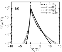
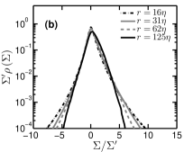
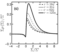
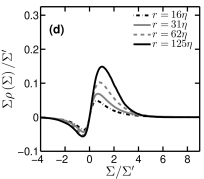
Figure 1: Top: probability density functions (PDFs) of $\Sigma$ in HIT2, normalised by the standard deviation $\Sigma^{\prime}$. (a) Gaussian filter. (b) Sharp filter. Bottom: weighted PDF, whose integral defines $\Phi_{F}$ and $\Phi_{B}$. (c) Gaussian filter. (d) Sharp filter.

We now move towards the dynamics of $\left\langle\Sigma\right\rangle$, based on its time series which we computed for all flows with a Gaussian filter - the sharp filter was used only on a few HIT fields widely spaced in time. They are shown on Fig. 2(a) at two filter widths, together with the kinetic energy $\left\langle K\right\rangle=\left\langle u_{i}u_{i}\right\rangle/2$ and the viscous dissipation $\left\langle\varepsilon\right\rangle$. It is clear that the signals are correlated, but that there is a delay separating them. $\left\langle K\right\rangle$ and $\left\langle\varepsilon\right\rangle$ behave as the earliest and latest signals, while the delay of $\left\langle\Sigma\right\rangle$ with respect to $\left\langle K\right\rangle$ increases with decreasing $r$.

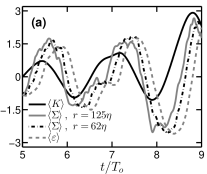
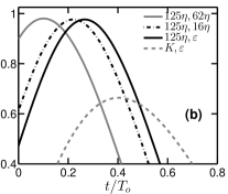
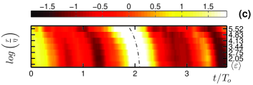
Figure 2: (a) Temporal evolution of spatially-averaged quantities, centered and normalized by their standard deviation; HIT2. (b) Cross-correlation curves between time series of $\left\langle\Sigma\right\rangle$ at various filter widths and between $\left\langle K\right\rangle$ and $\left\langle\varepsilon\right\rangle$; HIT2. (c) Time-scale diagram of $\left\langle\Sigma\right\rangle$, with $r$ decreasing from top to bottom and $\left\langle\varepsilon\right\rangle$ added as the bottom band; HIT3 with $r/\eta$ values from Table 2. The dash-dotted line corresponds to $\overline{\varepsilon}^{1/3}\Delta t=(250\eta)^{2/3}-r^{2/3}$ - see Eq. (6).

To visualize this effect more clearly, Fig. 2(c) displays the temporal evolution of $\left\langle\Sigma\right\rangle$ as a color map where the abscissae are time. Color bands corresponding to $\left\langle\Sigma\right\rangle$ have been ordered vertically with $r$ decreasing logarithmically downwards, and $\left\langle\varepsilon\right\rangle$ added at the bottom. The propagation across $r$ and $t$ of disturbances in $\left\langle\Sigma\right\rangle$ is evident. To quantify this process, we compute the temporal cross-correlation of all these signals with each other, as well as their temporal autocorrelation. A few such correlations are illustrated on Fig. 2(b), where the peak appears at the average delay between the two chosen signals. We start by looking at $\Delta t_{tot}$, the average time taken by a change in $\left\langle K\right\rangle$ to propagate and appear as a change in $\left\langle\varepsilon\right\rangle$. It is compiled in Table 1 for all our flows, which shows that $\Delta t_{tot}$ is approximately half the integral dissipation time $T_{o}\equiv\overline{K}/\overline{\varepsilon}$. Similar data are scarce in the literature, so that a comparison is not straightforward. In a computational study of homogeneous shear flow,Pumir (1996) the delay between the time histories of $\left\langle K\right\rangle$ and $\left\langle\varepsilon\right\rangle$ was estimated to be of the order of $\Delta t_{tot}/T_{o}\approx 1.5$ at $Re_{\lambda}\approx 50$. Since this disagrees with our $\Delta t_{tot}/T_{o}=0.49$ at $Re_{\lambda}\approx 107$, we repeated the simulation in Ref. Pumir, 1996, and found $\Delta t_{tot}/T_{o}=0.52$. The discrepancy can probably be attributed to the different estimation methods. Cross-correlations were not computed in Ref. Pumir, 1996, where $\Delta t_{tot}$ was not the main focus of the study. A value of $\Delta t_{tot}/T_{o}=0.44$ can be extracted from the data in Ref. Horiuti and Tamaki, 2013 where a DNS of HIT was ran at $Re_{\lambda}=122$, which agrees well with our findings. In Ref. Pearson et al., 2004, a $\Delta t_{tot}$ was defined as the delay between $\left\langle K\right\rangle^{3/2}/L_{int}$ and $\left\langle\varepsilon\right\rangle$, where $L_{int}=(3\pi/4\left\langle K\right\rangle)\int k^{-1}E(k){\,\rm d}k$. Using temporal cross-correlations in HIT at $Re_{\lambda}=219$ – comparable to our HIT2, they found $\Delta t_{tot}/T_{o}\approx 0.21$. We found $\Delta t_{tot}/T_{o}\approx 0.28$ using our HIT2 and the same definition of $\Delta t_{tot}$ as in Ref. Pearson et al., 2004, confirming that the lag between $\left\langle K\right\rangle^{3/2}/L_{int}$ and $\left\langle\varepsilon\right\rangle$ is shorter than that between $\left\langle K\right\rangle$ and $\left\langle\varepsilon\right\rangle$.

A comment on the origin of the time dependence of $\left\langle K\right\rangle$, $\left\langle\varepsilon\right\rangle$ and $\left\langle\Sigma\right\rangle$ is in order. The temporal oscillations of $\left\langle K\right\rangle$ and $\left\langle\varepsilon\right\rangle$ in HST are known to be physically caused and related to bursting .Pumir (1996) In the HIT simulations, the turbulence is sustained by a deterministic force

$$\hat{f}_{i}\left(\bm{k},t\right)=\begin{cases}\overline{\varepsilon}\hat{u}_{i}\left(\bm{k},t\right)/\left[2E_{f}(t)\right],&\text{if $0<k<k_{f}$},\\ 0,&\text{otherwise},\end{cases}$$ (3)

where $\overline{\varepsilon}$ is the target mean dissipation,Machiels (1997) $E_{f}(t)=\int_{0}^{k_{f}}E\left(k,t\right){\,\rm d}k$ and $k_{f}=4\pi/L_{x}$. This commonly used scheme is mildly unstable, because of the delay between $\hat{f}_{i}$ and $\left\langle\varepsilon\right\rangle$. It generates time oscillations of the energy while maintaining a constant resolution of $k_{max}\eta=1.5$ in the mean.

Table 3: Symbol legend for Figs. 3 and 5. $r_{a}/\eta=10a\sqrt{6}/\pi$ so that $r_{{}_{1}}\approx 8\eta$, $r_{{}_{2}}\approx 16\eta$, etc.

	$r\rightarrow\left\langle\varepsilon\right\rangle$	$a=1$	$a=2$	$a=4$	$a=8$	$a=16$
HST	+	$N/A$	$\times$	$\ast$	$\Diamond$	$N/A$
HIT1	$\square$	$\vartriangle$	$\Circle$	$\triangledown$	$N/A$	$N/A$
HIT2	$\color[rgb]{.5,.5,.5}\blacksquare$	$\color[rgb]{.5,.5,.5}\blacktriangle$	$\color[rgb]{.5,.5,.5}\CIRCLE$	$\color[rgb]{.5,.5,.5}\blacktriangledown$	$\color[rgb]{.5,.5,.5}\blacktriangleright$	$N/A$
HIT3	$\blacksquare$	$\blacktriangle$	$\CIRCLE$	$\blacktriangledown$	$\blacktriangleright$	$\blacktriangleleft$

With these two flows at hand, we can assess the dependence of $\Delta t_{tot}$ on the large-scale forcing. We define the characteristic time scale $T_{KK}$ of the kinetic energy as the width of the temporal autocorrelation of $\left\langle K\right\rangle$ at half its peak height. The ratio $T_{KK}/\Delta t_{tot}$ is between 2 and 2.5 for all our HIT simulations, but about 9 for the HST – see Table 1. Yet changes in $\left\langle K\right\rangle$ appear as changes in $\left\langle\varepsilon\right\rangle$ within half a large-eddy turnover time in the two differently forced flows, suggesting that $\Delta t_{tot}/T_{o}$ is a common feature of the energy cascade when the large scales fluctuate with periods in our range of $T_{KK}/T_{o}$. The dependence of our measured $\Delta t_{tot}/T_{o}$ on the large-scale period could be studied further by extending this range of $T_{KK}/T_{o}$ with the addition of a modulating frequency in the forcing, as done Ref. Kuczaj, Geurts, and Lohse, 2006, or with a stochastic forcing.Eswaran and Pope (1988)

We next test the additivity of the delay times. We want to see if the time taken by a disturbance in the energy flux in going from scale size $r_{3}$ to $r_{1}$ is equal to the sum of the delays in going from $r_{3}$ to $r_{2}$ and from $r_{2}$ to $r_{1}$, where $r_{3}>r_{2}>r_{1}$. Fig. 3(a) displays the average time needed for disturbances in the energy fluxes at a given scale $r$ to travel down to $\left\langle\varepsilon\right\rangle$. This time is computed for all available combinations of two intermediate jumps starting at $r$ and ending in $\left\langle\varepsilon\right\rangle$. The agreement between the different jump combinations within the same flow and across different flows is satisfactory. In order to highlight any residual discrepancy, we display the value of the ratios between one- and two-step cascading times on Fig. 3(b). A ratio close to unity implies additivity of the delays, which is confirmed for all the starting scales $r$ and flows examined. Note the narrow range of the vertical axis. Note also that Fig. 3(a) hints at two different regimes for $r$ above and below approximately $30\eta$. This is consistent with the results of Ref. Yoshida, Yamaguchi, and Kaneda, 2005, who showed that viscous eddies below $r/\eta\approx 30$ are enslaved to larger ones above that scale. In essence, $r/\eta=30$ is the lower limit of the inertial cascade.

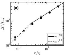
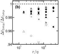
Figure 3: (a) Delay between $\left\langle\Sigma\right\rangle$ and $\left\langle\varepsilon\right\rangle$, measured either as the one-step delay, or as the sum of two intermediate steps involving $r_{a}$. (b) Ratio between two- and one-step delays. See Table 3 for symbols of $r_{a}$ and flow.

In an influential paper, Lumley discusses two cascade models,Lumley (1992) and proposes a forcing experiment similar to the present one to distinguish between them. He starts by considering a hierarchy of discrete eddies of decreasing size. In the first model, each eddy transfers its energy to the one immediately below. The transfer occurs at a rate determined by the corresponding scale-dependent eddy turnover time, $[k^{3}E(k)]^{-1/2}\sim k^{-2/3}\sim r^{2/3}$, so that the propagation of energy from the large towards the small scales develops into a front-like diffusion through scale-space with a finite scale-dependent velocity. In the second model, most of the energy is still transferred to the immediately smaller eddy below, but a fraction is passed to other eddies further along the cascade. Hence the smallest eddies receive a small amount of energy almost immediately after it is injected into the system, and increasing amounts as time goes on. The difference between the two models is that all the energy in the first one has to pass through each eddy size, resulting in additive cascade times, while this additivity is not guaranteed in the second model. Theoretical arguments were put forward both for and against long-range energy transfer,Yeung and Brasseur (1991); Domaradzki, Liu, and Brachet (1993) and attempts were made to carry out the forcing experiment, but they were hindered by the low Reynolds numbers available from simulations at the time. The matter has remained controversial until now, and our additive data on Fig. 3 favors the local model.

We now focus on the scaling of $\Delta t$. We start by introducing the strong assumption that the values of $\Delta t$ we measure are between scales $r$ within an inertial range, where $r$ and $\overline{\varepsilon}$ are the only relevant quantities. Within this simplistic framework, then, a velocity in $r$-space can be defined as

$$\dot{r}=\overline{\varepsilon}/\overline{\rho}_{{}_{E}},$$ (4)

where the energy density $\overline{\rho}_{{}_{E}}(r)$ is a real-space equivalent of $\overline{E}(k)$. We put forward the following candidate for $\overline{\rho}_{{}_{E}}$, based on $q=\widetilde{u}_{i}\widetilde{u}_{i}/2$:

$$\overline{\rho}_{{}_{E}}=-\frac{d\overline{q}}{dr}.$$ (5)

Other densities have been introduced in physical space. Townsend’s $r$-derivative of the correlation function, Townsend (1976) or the signature function found in Ref. Davidson and Pearson, 2005 are two examples. We chose our expression as it is based on the filtering approach we use. The data on Fig. 4(a) shows that the energy density $-d\overline{q}/dr$ in our two flows is a positive quantity. In Fig. 4(b) we see that the energy $-\Delta\overline{q}$ contained between $r$ and $r+\Delta r$ is a quantity which grows proportionaly to $r^{2/3}$ within a reasonable range in HIT3 - not so in HST with much smaller scale separation. Such $r^{2/3}$ behaviour is consistent with the Kolmogorov-Obukhov theory, Kolmogorov (1941); Obukhoff (1941) yet it is based on a completely different flow decomposition from the structure function.

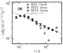
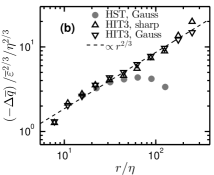
Figure 4: (a) Derivative of $\overline{q}=\overline{\widetilde{u}_{i}\widetilde{u}_{i}}/2$ with respect to $r$. The dashed line corresponds to $\overline{\varepsilon}^{2/3}r^{-1/3}$. (b) Energy content within a band of scales between $r$ and $r+\Delta r$, where $\Delta r$ goes from a given $r$ to the next bigger $r$ in the plotted series. $\Delta\overline{q}=\frac{1}{2}\overline{\widetilde{u}_{i}\widetilde{u}_{i}}(r+\Delta r)-\frac{1}{2}\overline{\widetilde{u}_{i}\widetilde{u}_{i}}(r)$.

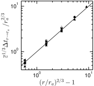
Figure 5: $\overline{\varepsilon}^{1/3}\Delta t_{r\rightarrow r_{a}}/r_{a}^{2/3}$ against $(r/r_{a})^{2/3}-1$, where $\Delta t_{r\rightarrow r_{a}}$ is the average delay between $\left\langle\Sigma(r)\right\rangle$ and $\left\langle\Sigma(r_{a})\right\rangle$, with $r>r_{a}$. Symbols as in Table 3. The solid line corresponds to Eq. (6)

Substituting $\overline{\rho}_{{}_{E}}$ in Eq. (4) by $\overline{\varepsilon}^{2/3}r^{-1/3}$, and integrating from $r_{a}$ to $r$ leads to

$$\Delta t_{r\rightarrow r_{a}}=\overline{\varepsilon}^{-1/3}\left(r^{2/3}-r^{2/3}_{a}\right),$$ (6)

which implies that our data should fall on a straight line when plotted logarithmically as done in Fig. 5. The agreement is not completely unsatisfactory. Particularly when considering the inertial range assumptions used which have no reason to apply if $r$ or $r_{a}$ are below the viscous limit of $30\eta$, or given the poor compliance of HST to the inertial range scaling with $r$ - see Fig. 4. A dashed line following Eq. (6) for HIT3 was added on Fig. 2(c).

A derivation of Eq. (6) carried out in spectral space can be found in Ref. Pope, 2000, leading to a $k^{-2/3}$ dependence of $\Delta t$. Ref. Wan et al., 2010 studied Lagrangian time correlations of $\Sigma(k)$ and $\varepsilon$, which hinted at a $k^{-2/3}$ dependence of the peaks in their correlations - see inset of their Fig. 2. Earlier, the same group measured the temporal correlation between the energy at a given scale and the energy at a smaller scale found later by following the flow in both forced and decaying HIT. Meneveau and Lund (1994) Their conclusion that the peak in correlation happens later for increasing scale separation is consistent with what we observe. A difficulty with that work was the use of correlations of energy rather than energy flux. Fluxes are the quantities conserved across cascades, and the natural objects for their study. Furthermore, they could only consider one-jump delays, ruling out the additivity test on Fig. 3 which supports the locality of the energy cascade in an average sense.