Time-Symmetric Rolling Tachyon Profile
Matheson Longton
Department of Physics and Astronomy
University of British Columbia
Vancouver, Canada

We investigate the tachyon profile of a time-symmetric rolling tachyon solution to open string field theory. We algebraically construct the solution of [1] at 6th order in the marginal parameter, and numerically evaluate the corresponding tachyon profile as well as the action and several correlation functions containing the equation of motion. We find that the marginal operator’s singular self-OPE is properly regularized and all quantities we examine are finite. In contrast to the widely studied time-asymmetric case, the solution depends nontrivially on the strength of the deformation parameter. For example, we find that the number and period of oscillations of the tachyon field changes as the strength of the marginal deformation is increased. We use the recent renormalization scheme of [2], which contains two free parameters. At finite deformation parameter the tachyon profile depends on these parameters, while when the deformation parameter is small, the solution becomes insensitive to them and behaves like previously studied time-asymmetric rolling tachyon solutions. We also show that convergence of perturbation series is not as straightforward as in the time-asymmetric case with regular OPE, and find evidence that it may depend on the renormalization constants.

1 Introduction and Conclusions

In a boundary CFT, the boundary condition can be deformed on any section of the boundary by exponentiating a marginal operator integrated along it, as in

$$e^{\lambda\int dt\,V(t)}~{}.$$ (1)

The marginal parameter $\lambda$ controls the strength of the deformation. In Open String Field Theory, allowed D-brane configurations are in one to one correspondence with classical solutions. The rolling tachyon is the time-dependent solution which corresponds to a decaying D-brane. There are two rolling tachyon solutions obtained by different marginal deformations of the D-brane CFT. The simpler case, the exponential rolling tachyon, involves the marginal operator $V(t)=e^{X^{0}(t)}$ and represents a D-brane which exists in the infinite past and then decays at a finite time. This case has been studied using level truncation methods [3, 4] as well as analytically [5, 6, 7], and is relatively simple because the OPE of the marginal operator with itself is finite. The more difficult case uses the time-symmetric marginal operator $V=\sqrt{2}\cosh(X^{0})$, which has the singular self-OPE $V(0)V(x)\sim\frac{1}{x^{2}}$. This rolling tachyon corresponds to placing a D-brane at $t=0$ and letting it decay at both $t=-\infty$ and $t=+\infty$.

In SFT, the tachyon profile is the tachyon component of the string field as a function of time. In the symmetric case it has the form

$$T(t)=2\sum_{n=1}^{\infty}\sum_{j=0}^{\left\lfloor n/2\right\rfloor}\lambda^{n}\beta_{n}^{(j)}\cosh((n-2j)t)~{},$$ (2)

where $\beta_{n}^{(j)}$ are coefficients which can be calculated numerically and $\left\lfloor n/2\right\rfloor$ is the greatest integer less than or equal to $n/2$, so that $n-2j\geq 0$. In this notation the deformation strength $\lambda$ is taken to be negative for physical solutions [5]. In the exponential case, $\lambda$ controls the time at which the D-brane decays, while for the time-symmetric case it determines the lifetime of the D-brane, with longer lifetimes corresponding to $\lambda$ closer to zero. In the regular OPE case, instead of the double sum and time-symmetric $\cosh$ functions, energy conservation tells us that there is only a single sum of exponentials involving coefficients with $\beta_{n}^{(0)}$:

$$T_{\text{reg}}(t)=\sum_{n=1}^{\infty}\lambda^{n}\beta_{n}^{(0)}e^{nt}~{}.$$ (3)

While the $\beta_{n}^{(j)}$ are in general gauge-dependent, for one choice of gauge it was proven that the sum in the regular OPE case converges for all $\lambda$, with the asymptotic behaviour $\beta_{n}^{(0)}\sim e^{-\gamma n^{2}}$ [7]. Numerical data suggests that this is true in other gauges as well, as shown in figure 3b. The trouble with this is that the tachyon profile itself exhibits wild oscillations which grow exponentially in magnitude, while the vacuum without any D-branes is a well defined and finite point in string field space. How these two very different looking string fields are reconciled has been the source of much speculation (see, for example, [8]). Our results confirm that the tachyon profile has the same growing oscillatory behaviour in the time-symmetric case, and do not appear to exclude any of the current hypotheses.

When studying the marginal operator $V=\sqrt{2}\cosh(X^{0})$ leading to the time-symmetric rolling tachyon, we must be careful to avoid singularities arising from the operator’s OPE. Analytic solutions for marginal deformations require the insertion of many copies of the marginal operator with separations that are integrated over, and there will be divergences when two operators approach each other. Fortunately there are several solutions which are intended to handle this issue [1, 9, 10, 11]. The most recent work, by Erler and Maccaferri, does not apply to solutions which have a non-trivial time direction, so we cannot use it for the rolling tachyon. Fuchs, Kroyter and Potting’s solution was designed with the photon marginal deformation in mind, but it is possible that it could describe the rolling tachyon as well. The solution of [10] is a generalization of [7] to operators with singular OPE, and it could be applied to the rolling tachyon. In fact it has been suggested that this solution could give the tachyon profile in the form (9), which would help settle the convergence issue.

Our focus, however, will be on the work of Kiermaier and Okawa. They proposed a general construction dependent on the existence of a suitable renormalization scheme [1], which was investigated and refined in [2]. A general renormalization scheme satisfying the necessary conditions was shown in [2] to have at least two free parameters, suggesting that the tachyon profile could have free parameters as well. Here we will perform the first explicit numerical calculations for this solution, and we will show that the tachyon profile is a finite function which does in fact depend on the free parameters.

When we implement the solution $\Psi$ of [1] with the renormalization scheme of [2] we can find the tachyon profile for the symmetric rolling tachyon. This involves algebraically constructing the wedge states with insertions corresponding to the solution, taking expectation values, and then performing the required integrals numerically. Here this is done up to 6th order in $\lambda$. It will have the form (2), where now the function is symmetric in $t$ and all the $\beta_{n}^{(j)}$ are non-zero. The marginal operator $\sqrt{2}\cosh(X^{0})$ contains the operators $e^{\pm X^{0}}$ with both signs, and the coefficients $\beta_{n}^{(j)}$ correspond to terms with $n-j$ factors of one of the two operators and $j$ factors of the other. Since renormalization has the effect of adding counterterms for collisions of operators with opposite sign, the $j=0$ coefficients involve no counterterms and behave very similarly to exponential solutions. These show the same $\beta_{n}^{(0)}\sim e^{-\gamma n^{2}}$ asymptotic behaviour, implying that the sum $\sum_{n=1}^{\infty}\lambda^{n}\beta_{n}^{(0)}\cosh(nt)$ converges absolutely for all $\lambda$. For $|\lambda|\ll 1$, as is the case when the D-brane survives for a long time, the $j>0$ coefficients are suppressed due to extra factors of $\lambda$. This results in a decay process which looks very much like the regular case, as the decay is well separated from the “anti-decay” by the D-brane’s lifetime. Once this lifetime is long enough, further shrinking $\lambda$ even has the same effect on the decay time as it would with the exponential rolling tachyon, simply shifting the time of the decay.

For the $\beta_{n}^{(j)}$ coefficients with $j>0$, each coefficient is calculated using a number of counterterms determined by $j$. The counterterms in turn are functions of the two parameters of the renormalization scheme, $C_{0}$ and $C_{1}$. The bulk coefficients are therefore polynomial functions of $C_{0}$ and $C_{1}$. Because these coefficients are not constants, patterns such as the asymptotic behaviour for $j=0$ could depend on the choice of $C_{0}$ and $C_{1}$. Considering only the $j=1$ coefficients, with $C_{0}=C_{1}=0$ they are quite a good fit to $\beta_{n}^{(1)}\sim e^{-\gamma_{1}(n-2)^{3}}$. In fact there is no choice of those constants for which the exponential quadratic behaviour $\beta_{n}^{(1)}\sim e^{-\gamma_{1}(n-2)^{2}}$ fits as closely. This suggests that the sum $\sum_{n=2}^{\infty}\lambda^{n}\beta_{n}^{(1)}\cosh((n-2)t)$ also converges, but there may still be some choices of $C_{0}$ and $C_{1}$ for which this is not the case, or for which the radius of convergence in $\lambda$ is finite. For example, choosing the constants so that $\beta_{n}^{(1)}$ are a best fit to the exponential cubic behaviour results in $\beta_{n}^{(2)}$ which are increasing, at least for the three coefficients we can calculate with $j=2$.

So how does the inclusion of all the $\beta_{n}^{(j)}$ coefficients affect the shape of the tachyon profile? We show that for $|\lambda|\ll 1$ these coefficients are negligible, but as the D-brane lifetime is decreased there comes a point where more coefficients must be considered. Some terms cease to dominate for any range of time, and the number of oscillations actually decreases. The missing oscillation means that the effective “period” is significantly decreased. What this means physically is not clear, since the period is a gauge dependent quantity related to the coefficient $\gamma$ in the exponent of the asymptotic behaviour. The tachyon profile for small $\lambda$ is very similar to that of [5], while for large $\lambda$ it has features similar to the tachyon profile of [7], so perhaps the solution is interpolating between regular-OPE solutions in different gauges as the marginal deformation strength is changed. Understanding this phenomenon is left for future work.

This paper is organized as follows. Section 2 is focused on the details of the tachyon profile, and contains discussion and plots of results. In section 3 we briefly discuss how the numerical calculations were performed, and demonstrate that our results converge to appropriate values. There we also discuss sources of roundoff error which can influence the calculations.

2 The Tachyon Profile

The solution of [1] presents a promising framework for construction of a time-symmetric rolling tachyon solution, but it was not applied to any specific marginal deformation. Taking that approach and inserting the marginal deformation $V=\sqrt{2}\cosh(X^{0})$ we are able to numerically compute the tachyon profile up to 6th order in the deformation parameter $\lambda$. Since the tachyon profile has previously been calculated for several exponential rolling tachyon solutions, we can compare our results in order to determine what qualitative differences appear in the time-symmetric case. It is also useful to have explicit numerical evidence that the renormalization scheme studied in [2] is effective and the solution remains finite despite the singular OPE that the marginal operator has with itself.

The solution takes the form of a wedge state with insertions on the boundary. While one insertion will always be at a fixed location, the rest are integrated. The renormalization procedure replaces pairs of operators with appropriate counterterms under the integral. Each operator $V$ contains two terms carrying $\pm 1$ unit of “momentum” in the time direction, but the counterterms are functions and carry no momentum. In (2) the coefficient $\beta_{n}^{(j)}$ clearly contains the part of the tachyon profile with $n$ factors of $\lambda$ and $k=n-2j$ units of this momentum, so it follows that the coefficients $\beta_{n}^{(0)}$ contain no counterterms. This is as it should be since operators $e^{\pm X^{0}}$ with the same sign have a regular OPE; the singular OPE of the $\cosh(X^{0})$ marginal operator comes entirely from the collision of exponentials with opposite sign. The index $j$, which counts the momentum deficit, also has the effect of counting the maximum number of counterterm factors. For the coefficients $\beta_{n}^{(j)}$, table 1 shows their values as calculated by the Cuhre algorithm, and with the exception of two terms we will use those coefficients. For technical reasons explained in section 3.3, the two terms marked with asterisks will use values found by the Suave algorithm instead, and those are shown in table 2. Occasionally we will want to think of the tachyon profile in terms of these timelike momentum modes, and write

$$T(t)=\sum_{k=0}^{\infty}2\cosh(kt)\sum_{n=k}^{\infty}\lambda^{n}\beta_{n}^{\left(\frac{n-k}{2}\right)}~{}.$$ (4)

This form is equivalent to (2) as long as we define $\beta_{n}^{(j)}$ to vanish for non-integer $j$, as well as for $n=j=0$.

$n$	$j$	$\beta_{n}^{(j)}$
1	0	$\frac{1}{\sqrt{2}}$
2	1	$(-1.29904\ldots\pm 3\cdot 10^{-11})+(0\pm 1\cdot 10^{-14})C^{L}$
2	0	$(0.0760297\ldots\pm 8\cdot 10^{-16})$
3	1	$(-1.30572\pm 4.3\cdot 10^{-5})-(0.707107\ldots\pm 3\cdot 10^{-14})C_{1}-(0\pm 2\cdot 10^{-4})C^{L}$
3	0	$(9.150\pm 0.019)\cdot 10^{-4}$
4	2	$(0.655579\pm 6\cdot 10^{-6})+(0\pm 3\cdot 10^{-4})C^{L}+(3.2858\pm 0.0021)C_{1}+(4.9\pm 7.8)\cdot 10^{-15}C^{L}C_{1}$
		$\quad+(0\pm 1\cdot 10^{-3})C_{0}+(0\pm 1\cdot 10^{-14})C^{L}C_{0}$
4	1	$-(0.4488\pm 0.0031)+(0\pm 8\cdot 10^{-4})C^{L}-(0.2349\pm 0.0023)C_{1}+(1.4\pm 0.7)\cdot 10^{-7}C_{0}$
4	0	$(1.17222\pm 0.00013)\cdot 10^{-6}$
5	2	$(0.723\pm 0.011)+(0\pm 1\cdot 10^{-3})C^{L}+(4.387\pm 0.041)C_{1}+(0\pm 0.02)C^{L}C_{1}+(3.53553\ldots\pm 7\cdot 10^{-15})C_{1}^{2}$
		$\quad+(0\pm 6\cdot 10^{-3})C_{0}+(0\pm 0.01)C^{L}C_{0}$
5	1	$(-0.01221\pm 1.2\cdot 10^{-4})+(0\pm 2\cdot 10^{-5})C^{L}-(5.86\pm 0.34)\cdot 10^{-3}C_{1}-(1.27\pm 0.61)\cdot 10^{-4}C_{0}$
5	0	$(1.598\pm 0.007)\cdot 10^{-10}$
6	3	$(-0.3\pm 0.4)^{*}+(0\pm 3\cdot 10^{-3})C^{L}-(2.572\pm 0.026)C_{1}+(0.3\pm 1.2)\cdot 10^{-3}C^{L}C_{1}-(23.9401\pm 0.0013)C_{1}^{2}$
		$\quad+(1.5\pm 3.1)\cdot 10^{-14}C^{L}C_{1}^{2}+(0.0955\pm 0.0030)C_{0}+(0\pm 5\cdot 10^{-3})C^{L}C_{0}-(0.135\pm 0.015)C_{0}C_{1}$
		$\quad-(1.2\pm 3.9)\cdot 10^{-14}C^{L}C_{0}C_{1}+(5.8\pm 1.5)\cdot 10^{-6}C_{0}^{2}$
6	2	$(0.4991\pm 0.0050)+(0.4\pm 1.3)\cdot 10^{-5}C^{L}+(1.912\pm 0.019)C_{1}+(0.8\pm 4.1)\cdot 10^{-3}C^{L}C_{1}+(1.715\pm 0.024)C_{1}^{2}$
		$\quad+(1.879\pm 0.025)\cdot 10^{-2}C_{0}+(0\pm 2\cdot 10^{-3})C^{L}C_{0}+(4.77\pm 0.38)\cdot 10^{-2}C_{0}C_{1}-(2.37\pm 0.09)\cdot 10^{-7}C_{0}^{2}$
6	1	$(-2.686\pm 0.027)\cdot 10^{-5}-(1.6\pm 5.9)\cdot 10^{-8}C^{L}-(9.1\pm 2.2)\cdot 10^{-6}C_{1}-(7.3\pm 0.7)\cdot 10^{-7}C_{0}$
6	0	$(2.18\pm 0.04)\cdot 10^{-15\,*}$

Table 1: The non-zero coefficients $\beta_{n}^{(j)}$ of the tachyon profile for the $\cosh$ rolling tachyon with singular self-OPE. Cuhre/QAG results shown. The constant $C^{L}$ is part of the renormalization scheme of [2], but it can not influence the solution, so we safely set it to zero in our analysis. $C^{L}$ was included in these numerical results only to demonstrate that it does not contribute to the solution at all.
^∗ These two coefficients found using the Cuhre algorithm appear to be unreliable, so the corresponding Suave results in table 2 will be used for analysis instead.

$n$	$j$	$\beta_{n}^{(j)}$
1	0	$\frac{1}{\sqrt{2}}$
2	1	$-(1.2985\pm 0.0003)-(4.134\pm 0.007)\cdot 10^{-6}C^{L}$
2	0	$(7.61\pm 0.07)\cdot 10^{-2}$
3	1	$-(1.301\pm 0.005)-(0.001\pm 0.010)C^{L}-(0.707107\ldots\pm 7\cdot 10^{-18})C_{1}$
3	0	$(8.99\pm 0.09)\cdot 10^{-4}$
4	2	$(0.659\pm 0.007)+(0.2\pm 2.6)\cdot 10^{-3}C^{L}+(3.288\pm 0.003)C_{1}+(0\pm 1\cdot 10^{-17})C_{1}C^{L}+(0.5\pm 3.4)\cdot 10^{-3}C_{0}$
		$\quad+(0\pm 5\cdot 10^{-9})C_{0}C^{L}$
4	1	$-(0.449\pm 0.004)-(0.1\pm 1.4)\cdot 10^{-3}C^{L}-(0.235\pm 0.002)C_{1}+(1.39\pm 0.07)\cdot 10^{-4}C_{0}$
4	0	$(1.163\pm 0.002)\cdot 10^{-6}$
5	2	$(0.722\pm 0.012)+(1.3\pm 1.3)\cdot 10^{-3}C^{L}+(4.38\pm 0.04)C_{1}+(0.014\pm 0.034)C_{1}C^{L}+(3.53553\ldots\pm 3\cdot 10^{-8})C_{1}^{2}$
		$\quad+(0.1\pm 6.5)\cdot 10^{-3}C_{0}-(0.3\pm 1.3)\cdot 10^{-2}C_{0}C^{L}$
5	1	$-(1.21\pm 0.01)\cdot 10^{-2}+(2.2\pm 1.1)\cdot 10^{-5}C^{L}-(5.81\pm 0.06)\cdot 10^{-3}C_{1}-(1.17\pm 0.01)\cdot 10^{-4}C_{0}$
5	0	$(1.27\pm 0.01)\cdot 10^{-10}$
6	3	$-(0.307\pm 0.004)-(1.6\pm 2.9)\cdot 10^{-3}C^{L}-(2.55\pm 0.05)C_{1}+(0.5\pm 3.6)\cdot 10^{-2}C_{1}C^{L}-(23.943\pm 0.008)C_{1}^{2}$
		$\quad+(0\pm 1\cdot 10^{-17})C_{1}^{2}C^{L}+(9.5\pm 0.5)\cdot 10^{-2}C_{0}-(8.0\pm 6.6)\cdot 10^{-3}C_{0}C^{L}-(0.12\pm 0.02)C_{0}C_{1}$
		$\quad+(0\pm 1\cdot 10^{-17})C_{0}C_{1}C^{L}+(5.0\pm 4.4)\cdot 10^{-5}C_{0}^{2}$
6	2	$(0.497\pm 0.005)-(2.1\pm 1.1)\cdot 10^{-4}C^{L}+(1.92\pm 0.02)C_{1}-(1.7\pm 2.6)\cdot 10^{-3}C_{1}C^{L}+(1.718\pm 0.013)C_{1}^{2}$
		$\quad+(1.774\pm 0.014)\cdot 10^{-2}C_{0}-(1.2\pm 2.3)\cdot 10^{-3}C_{0}C^{L}+(4.71\pm 0.05)\cdot 10^{-2}C_{0}C_{1}-(1.156\pm 0.016)\cdot 10^{-4}C_{0}^{2}$
6	1	$-(2.54\pm 0.02)\cdot 10^{-5}-(3.5\pm 0.3)\cdot 10^{-8}C^{L}-(1.222\pm 0.012)\cdot 10^{-5}C_{1}-(7.618\pm 0.014)\cdot 10^{-7}C_{0}$
6	0	$(2.3\pm 0.3)\cdot 10^{-15}$

Table 2: The non-zero coefficients $\beta_{n}^{(j)}$ of the tachyon profile for the $\cosh$ rolling tachyon with singular self-OPE. Suave results shown for comparison with the deterministic results of table 1.

The tachyon profile for several different solutions with regular OPE has been calculated before. It has the simpler form of $T(t)=\sum_{n=0}^{\infty}\lambda^{n}\beta_{n}\sqrt{2}^{n}e^{nt}$ where the coefficients $\beta_{n}\overset{\text{def}}{=}\beta_{n}^{(0)}$ are only non-zero for maximal momenta. In table 3 we compare the coefficients for those solutions to the ones we have found. We have changed the normalization of their coefficients by $2^{-\frac{n}{2}}$ for better comparison with our coefficients, due to the relative normalizations of the marginal operators $e^{X^{0}}$ and $\sqrt{2}\cosh(X^{0})$. Our coefficients show very similar falloff to [5] as $n$ is increased, though we do not expect exact agreement between any of the sets of coefficients because the tachyon profile is a gauge dependent quantity. We believe that each of these lists is related to the others by such gauge transformations, but constructing them is beyond the scope of this work.

	[5]	[7]	[3]	$\Psi$ here
$n$	$\beta_{n}$
1	$\frac{1}{\sqrt{2}}$	$\frac{1}{\sqrt{2}}$	$\frac{1}{\sqrt{2}}$	$\frac{1}{\sqrt{2}}$
2	0.0760295	0.290	0.0760297	0.0760297
3	$7.59312\cdot 10^{-4}$	0.0506	$7.732\cdot 10^{-4}$	$9.149\cdot 10^{-4}$
4	$6.54812\cdot 10^{-7}$	$4.18\cdot 10^{-3}$	$9.8145\cdot 10^{-7}$	$1.173\cdot 10^{-6}$
5	$4.93424\cdot 10^{-11}$	$1.54\cdot 10^{-4}$	$8.734\cdot 10^{-11}$	$1.275\cdot 10^{-10}$
6	$3.50136\cdot 10^{-16}$	$2.45\cdot 10^{-6}$	$7.903\cdot 10^{-13}$	$2.26\cdot 10^{-15}$
7	$2.41180\cdot 10^{-22}$	$1.64\cdot 10^{-8}$

Table 3: The coefficients for the tachyon modes of a purely exponential rolling tachyon with regular self-OPE. Calculated from the solutions of [5], [7], and [3]. The $n=k$ coefficients for our calculations based on [1] are included for comparison.

As in [5], we take $\lambda$ to be negative in order to study physical solutions. With this assumption, the tachyon profile (2) can be rewritten as

$$T(t)=\sum_{n=1}^{\infty}\sum_{j=0}^{\left\lfloor n/2\right\rfloor}(-1)^{n}\beta_{n}^{(j)}\left(e^{n(\ln|\lambda|+t)-2jt}+e^{n(\ln|\lambda|-t)+2jt}\right)~{},$$ (5)

where in practice the sum over $n$ only runs up to some cutoff $N$ where the coefficients can be computed. When only the $j=0$ coefficients and the first term in parentheses are considered, as in the regular OPE case, we can clearly see that a change of $\ln|\lambda|$ will only shift the time of the D-brane decay. For the singular case, however, the tachyon profile will have a different shape depending on the strength of the marginal deformation, controlled by $\ln|\lambda|$. The renormalization scheme also contains the constants $C_{0}$ and $C_{1}$, which will appear nontrivially in $\beta_{n}^{(j)}$ with $j>0$.

2.1 Small $\lambda$

We begin our analysis with the case $|\lambda|\ll 1$, where only the coefficients $\beta_{n}^{(0)}$ need to be considered. Following the notation of [5, 7], we will refer to these coefficients as $\beta_{n}\overset{\text{def}}{=}\beta_{n}^{(0)}$. We will focus on (5), which receives significant contributions from the first term in parentheses when $t>0$ and from the second term when $t<0$. Knowing that $T(t)$ is an even function, we will assume $t>0$ and not need to consider the second term. Since we are considering $-1\ll\lambda<0$, each term in the sum of (5) will be suppressed by the exponential until $t$ is large compared to $-\ln|\lambda|$. For a large fixed $t$, terms with $j>0$ will be small relative to others, so only the $j=0$ coefficients need to be considered. Since this is the case, the tachyon profile does not depend on the renormalization constants $C_{0}$ and $C_{1}$ at all. This had to be the case since there is no renormalization when all of the marginal operators have momentum in the same direction. We can then unambiguously plot the tachyon profile for small $|\lambda|$. In figure 1 we see $\ln|T(t)|$ for $\ln|\lambda|=-4$. Each “peak” represents the range of $t$ for which $T(t)$ is dominated by a specific exponential in the sum. For different values of $|\lambda|$ the shape of the oscillating part of the tachyon profile remains unchanged, and the whole half-plot shifts horizontally, with the size of the plateau in the middle changing as expected.

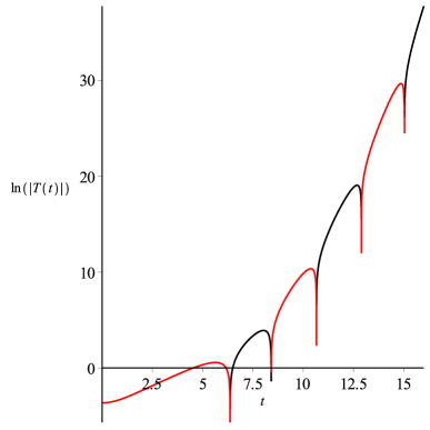
(a)

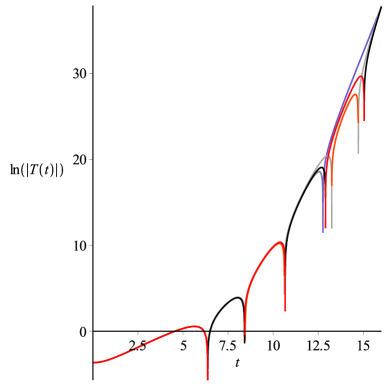
(b)

Figure 1: The tachyon profile $T(t)$ with only the $\beta_{n}^{(0)}$ coefficients considered. This is plotted for $\ln|\lambda|=-4$, where the approximation is valid. a) Black is for positive values of $T(t)$ and red is for negative values. b) The tachyon profile with all Suave coefficients from table 2 is also shown in orange and grey, and where the Cuhre-only results deviate is indicated with a blue line. We can see that the Suave results are qualitatively equivalent to the ones we use.

The size of the plateau which describes the time when the D-brane exists can be estimated by the time of the first zero of the tachyon profile. This time is plotted in figure 2a, and is linear for the region where $|\lambda|\ll 1$ is valid. The slope is $-1$ as it had to be from (5) when $t$ is significantly larger than $0$. We can also examine the “period” of the oscillations. The oscillations result from each exponential overtaking the one before, so we can calculate an estimate of their spacing by setting adjacent terms to be equal.

$$\beta_{n}e^{n(\ln|\lambda|+t_{n})} =\beta_{n+1}e^{(n+1)(\ln|\lambda|+t_{n})}$$ (6a)

$$t_{n} =-\ln|\lambda|+\ln\left(\frac{\beta_{n}}{\beta_{n+1}}\right)$$ (6b)

$$\Delta t_{n} =\ln\left(\frac{(\beta_{n})^{2}}{\beta_{n-1}\beta_{n+1}}\right)$$ (6c)

While there is no reason to expect this a priori, let us suppose that $\Delta t$ is a constant. In this case we have

$$\frac{\beta_{n+1}}{\beta_{n}}=e^{-\Delta t}\frac{\beta_{n}}{\beta_{n-1}}~{},$$ (7a)

which is a recursion relation with the solution

$$\beta_{n}\propto\rho^{n}e^{-\frac{n^{2}}{2}\Delta t}~{}.$$ (7b)

The factor $\rho^{n}$ can always be removed by taking $\beta_{n}^{(j)}\rightarrow\frac{\beta_{n}^{(j)}}{\rho^{n}}$ and simultaneously $\lambda\rightarrow\lambda\rho$, which does not alter the tachyon profile. In one particular solution for the rolling tachyon with regular OPE, Kiermaier, Okawa, and Soler [7] found that their solution’s coefficients had the asymptotic behaviour

$$\beta_{n}\sim e^{-\gamma n^{2}+O(n\ln n)}~{},$$ (8)

and in [6] it was shown that a solution equivalent to the one in [5] has coefficients which closely fit $b_{n}\sim e^{-\gamma n^{2}}$ without significant corrections. We have just shown that this same recurring pattern can be derived from the assumption of exponentially growing oscillations with constant period. In figure 3 we see the best fit lines for our $j=0$ coefficients, as well as those of several other known solutions, to the form $\beta_{n}\sim e^{-\gamma n^{2}}$. This was only predicted to be a fit for one solution at large $n$, but we see good agreement in all cases, even with $n$ never rising past 6 or 7 for any of the solutions considered. In figure 3a the fit is to the deterministic results of table 1 for $n\leq 5$ and the Suave result for $n=6$, but the Suave results with smaller $n$ are shown as the red points for reference. The Cuhre value for $\beta_{6}^{(0)}$ cannot be shown on a logarithmic plot since it has the wrong sign. It is curious that the coefficients fall so close to the $e^{-\gamma n^{2}}$ lines without any correction, even such as choosing $\rho\neq 1$ in (7b). While this trend was derived in our case from a constant period of oscillation, if it holds at higher $n$ it guarantees that the edge coefficients are a convergent series. The fact that all of the solutions appear to behave similarly suggests that they are also all convergent.

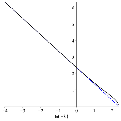
(a)

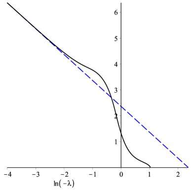
(b)

Figure 2: The time of the first zero of the tachyon as a function of $\ln|\lambda|$. An approximation to the asymptotic behaviour is shown as a dashed line. a) Only the $\beta_{n}^{(0)}$ coefficients are considered, so the plot is not valid for large $|\lambda|$. b) The whole tachyon profile is considered with coefficients from the fit of figure 4a.

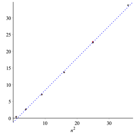
(a)

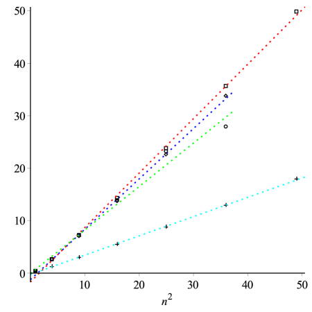
(b)

Figure 3: The falloff of the edge coefficients shown as $-\ln\beta_{n}^{(0)}$ versus $n^{2}$. A linear graph indicates that $\beta_{n}\propto e^{-\gamma n^{2}}$ holds, with $\gamma$ given by the slope. The best linear fit is also shown. a) The solution shown here, with slope $0.9599$. Red points are Suave values. b) Our solution as well as the other three presented in table 3. Square points are for [5], crosses are for [7], and circles for [3].

2.2 Large $\lambda$

Once we loosen the $|\lambda|\ll 1$ restriction, we must consider all of the coefficients $\beta_{n}^{(j)}$ and search for patterns there. Due to the small number of coefficients, and particularly the small number of rows with constant $j$, it is not possible to get a good understanding of any patterns or asymptotics for these coefficients, but we can speculate as to possible trends. The first thing we notice from table 1 is that the sign of the coefficients appears to alternate as $(-1)^{\frac{j}{2}}$. This is not strictly true even for the coefficients we have calculated, however, as choosing non-zero $C_{0}$ and especially $C_{1}$ will alter many of the coefficients and can affect their sign. With only a small number of the coefficients known, we do not know whether the large $n$ asymptotics are fixed or can be changed by a choice of the two free parameters. We can, however, attempt to force a few patterns and see which appear more naturally.

As a first choice we pick $C_{0}=C_{1}=0$ and notice that the $j=1$ coefficients appear to be a good fit to $\beta_{n}^{(1)}\sim e^{-\gamma_{1}k^{3}}$ with $k=n-2j$, which is shown in figure 4a. While this can be made to fit even better by a choice of renormalization constants, this would lead to some of $\beta_{n}^{(2)}$ being less than zero or to that row having increasing magnitudes. On the other hand, if we attempt to pick renormalization constants which are a fit to $\beta_{n}^{(1)}\sim e^{\gamma_{1}k^{2}}$, as shown in figure 4c, we do not find as good a fit. The same is true of $\beta_{n}^{(1)}\sim e^{\gamma_{1}n^{2}}$ using $n$ instead of $k$ in the exponent. It appears that the $j=1$ coefficients have a tendency towards the cubic exponential decay, while for $j=2$ we lack enough points to reach any conclusions. The red points in figure 4 again represent the Suave coefficients, and we see that $\beta_{n}^{(2)}$ have significantly different values once the renormalization constants are changed, but a look at table 2 suggests that this is mainly due to large errors in the Suave coefficients, so it is unlikely that the deterministic plots would change significantly if more sample points were used.

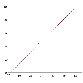
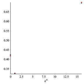
(a)

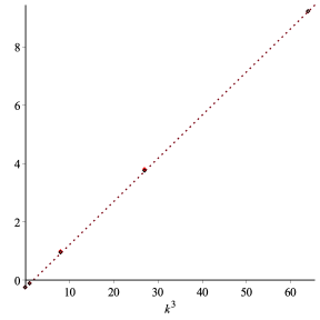
(b)

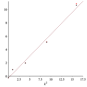
(c)

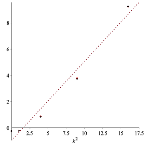
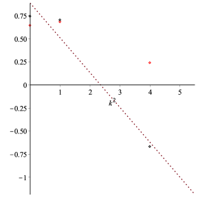
(d)

Figure 4: $\ln|\beta_{n}^{(j)}|$ plotted vs. functions of $k=n-2j$ with several different choices for $C_{0}$ and $C_{1}$. Black points are Cuhre values while red points are from the Suave algorithm. In a) we set $C_{0}=C_{1}=0$ and plot $j=1$ coefficients on the left and $j=2$ on the right. The $j=1$ coefficients with $C_{0}$ and $C_{1}$ optimized for the best linear fit appear in b), and c) attempts the same linear fit assuming a $k^{2}$ horizontal axis rather than $k^{3}$. d) attempts a linear fit to both the $j=1$ and $j=2$ sets of coefficients assuming a $k^{2}$ horizontal axis, with $j=1$ coefficients on the left and $j=2$ on the right.

While five points is not a lot of data, the $\beta_{n}^{(1)}$ coefficients suggest that each row with constant $j$ may eventually be a convergent series for at least some choice of renormalization constants. Showing that the full tachyon profile converges when these rows are added together, however, remains impossible until much higher order calculations can be performed. In particular, the large dependence of coefficients such as $\beta_{6}^{(3)}$ on $C_{1}$ is troubling since it suggests that if that constant is of order 1 then the sequence $\beta_{n}^{\left(\frac{n-k}{2}\right)}$ with constant $k$ could have increasing magnitudes. Thinking of (4) as

$$T(t)=2\sum_{k=0}^{\infty}\beta_{\text{eff}}^{(k)}(\lambda)\,\cosh(kt)~{},$$ (9)

the effective coefficients $\beta_{\text{eff}}^{(k)}(\lambda)$ would then be defined by series which do not converge for non-zero renormalization constants. Looking at table 1, even with vanishing renormalization constants, the magnitudes of the terms $\beta_{2j}^{j}$ do not drop off very fast, but with alternating sign the series may still converge.

Now that we have seen what the bulk coefficients look like, we can begin examining the tachyon profile for larger values of $|\lambda|$. Of course as we do this we must be aware that we are missing all coefficients $\beta_{n}^{(j)}$ with $n\geq 7$, and as we increase the strength of the marginal deformation those coefficients will begin to play a larger role, but we can still get a qualitative idea of the impact of the bulk coefficients on the tachyon profile. Since none of the optimized fits in figure 4 were significantly better than simply setting the renormalization constants to zero, we will choose that from now on. Other reasonable choices will not give results that are qualitatively different. For large negative $\lambda$ we see a tachyon profile in figure 5 with fewer oscillations than we had with just the edge coefficients from figure 1. As $|\lambda|$ decreases, the additional oscillation appears at $\ln|\lambda|\approx-1.948$. Once $\ln|\lambda|\lesssim-2.5$ the profile has stabilized and the plateau continues growing as $|\lambda|$ shrinks, just as we know it should from our discussion of the tachyon profile for small $|\lambda|$. The disappearance of this oscillation for large $|\lambda|$ is because the bulk coefficients cannot be neglected in this region, and they change the effective coefficients in (9).

The behaviour we see for these large values of $|\lambda|$ is not unprecedented; in [7] the tachyon profile had coefficients (seen in table 3) which did not decrease as quickly as other time-asymmetric solutions. That tachyon profile had fewer oscillations for all $\lambda$ because some of the exponentials did not dominate for any range of time. Aside from the obvious, that the singular OPE case is a symmetric function where the D-brane exists for a limited time while with regular OPE it exists until it decays at a finite time, the qualitative difference between the tachyon profiles seems to be that the period and number of oscillations can change this way. Because the strong deformation tachyon profile we have found is similar to the profile of [7], it suggests that changing the strength of the marginal deformation in the time-symmetric case is much like changing gauge in the time-asymmetric case. If the late time behaviour is equivalent to the tachyon vacuum under a time-dependent gauge transformation, as has been hypothesized [3], then in this case the gauge transformation should depend on both time and the marginal parameter in a non-trivial way. That our solution appears qualitatively like time-asymmetric ones for both weak and strong deformation parameter suggests that such gauge transformations remain a valid explanation of the oscillations in the time-symmetric case.

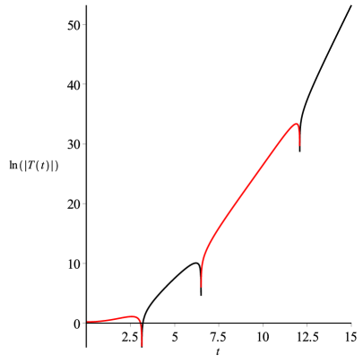
(a)

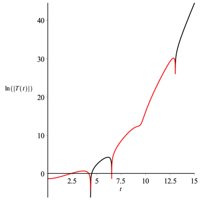
(b)

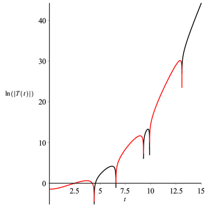
(c)

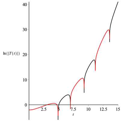
(d)

Figure 5: The log of the tachyon profile at a) $\ln|\lambda|=-0.5$, b) $\ln|\lambda|=-1.92$, c) $\ln|\lambda|=-1.98$, and d) $\ln|\lambda|=-2.5$. Positive values represented by black, negative values by red. The renormalization constants $C_{0}$ and $C_{1}$ are both set to zero.

3 A Few Technical Details

The solution and necessary renormalized operators have been defined in [1] and [2], so it is possible to numerically compute many quantities up to a reasonable accuracy. We use Maple to algebraically manipulate wedge states with insertions and produce functions to be integrated. This means writing routines for the star product, BRST operator, and correlation functions, among other things. While the number of terms grows extremely fast, it is possible to algebraically construct the solution up to 7th order in $\lambda$. The integrands produced, however, are complicated enough that I was only able to compile them for integration up to 6th order. Although the algebraic construction of the wedge states with insertions is a lengthy process, it is an exact one which should not produce any numerical errors. Evaluating the resulting integrals, however, is done by sampling the integrand at many points and estimating a result, and this process unavoidably introduces errors.

The integration is handled by off-the-shelf C++ routines. The CUBA library appears to be a good choice in most cases [12]. It is a collection of four algorithms for multi-dimensional numerical integration, three of which use pseudo-random sampling while the fourth is a deterministic algorithm. Since we are working at sixth order in $\lambda$ and the solution has ghost number one (corresponding to the number of fixed moduli), there are never more than five integrated coordinates in a given integral. While Monte Carlo algorithms do scale better as the dimension rises, in five or less dimensions it appears that the deterministic algorithm, Cuhre, is slightly more efficient. As we will see, Cuhre is also more reliable in most cases. Unfortunately, it only integrates functions of more than one variable, so in the one-dimensional case we use the QAG routine from the GNU scientific library. Each of the routines in the CUBA and GNU libraries provides its own error estimate, and the CUBA library routines also provide a chi-square estimate of the probability that the error is sufficient.

A single quantity to be calculated numerically, such as an individual term in the tachyon profile of table 1 or in one of the consistency checks of tables 6 and 7, generally consists of a small number of integrals. Each integral contains all of the terms in the solution which are integrated over a given number of coordinates, or equivalently all of the terms with the same number of integrated operators. Most quantities are the sum of two integrals, but a few are only a single integral, and quantities in the action can consist of more than two.

3.1 Convergence

In order to get as much data as possible, the collection of integrals we look at here will include all of the ones used in calculating the tachyon profile as well as the action and several components of the equation of motion. The action and equation of motion will be discussed as checks of consistency in section 3.3.

It is difficult to study convergence of the one-dimensional integrals due to the fact that the QAG algorithm does not report the number of samples used. We can, however, take several full sets of data for these integrals and compare the different calculations of the same integrals. We find that they all agree with each other well within the error estimates. The only troubling one-dimensional case is that of a constant integrand. This can be seen in the kinetic energy of the solution at fourth order in $\lambda$, which is the particularly simple quantity $\int_{0}^{1}dt~{}\frac{3}{2}-\frac{3}{2}$. The integration algorithm performs operations on the constant causing tiny roundoff errors which, when the constant value is subtracted, causes the result to differ from zero. This would not be a problem except that error analysis in numerical integration is based on variation of the integrand, and as such gives an estimated error which is extremely small. While in principle error estimates should account for the roundoffs inherent in their algorithm, in practice this does not seem to be the case. The error estimate becomes small enough that the reported result can actually be incorrect, and even unstable with respect to changing the desired accuracy. Most integrands worth using a numerical algorithm to integrate undoubtedly vary enough that this is not normally an issue. This is the only instance of such a problem that we encounter, but since the integral is trivial we do not need to rely on numerical integration for its value.

We now turn our attention to the Cuhre algorithm, so we will only be considering integrals over two or more dimensions. The first question we will ask here is whether the error bars reported by the integration algorithms are sufficient. Because we do not know the correct results for most of the integrals, we evaluate each integral with at least three different choices for the sample size, $N$. Making the assumption that the calculation with the largest $N$ is “correct”, we can compare the difference between each computed integral and the most accurate one to the error estimate reported by that integral. This is shown in figure 6a, where blue points have sufficient error bars and green points are within twice the error bars. The few red points are the outliers which differ from their largest $N$ partners by more than twice their error estimates. In a moment we will compare every computed integral with other calculations of the same integral, so the red points here will also have greater than $2\sigma$ difference in that comparison. Many of these points come from the same integrals, so there are actually not very many integrals which will need to be examined in detail. Our choice to prefer the Cuhre algorithm over the adaptive Monte Carlo algorithm Suave is justified by figure 6b, where we see that the Suave algorithm is as likely as not to underestimate the error. In its defence, Suave frequently reports a 100% $\chi^{2}$ estimate that the reported error is insufficient, but this is not particularly helpful in finding accurate values.

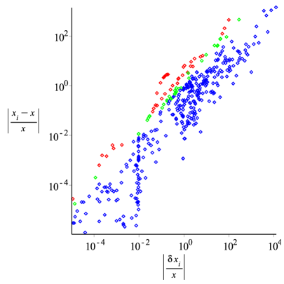
(a)

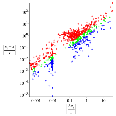
(b)

Figure 6: Plots showing the reliability of error estimates. The vertical axis is the difference of two calculations relative to the more precise of the two, and the horizontal axis is the relative error reported by the numerical integration. The Cuhre algorithm results are shown in a) and Suave results are in b). Points with differences greater than twice the reported errors are red, those with differences between one and two times the error are green, and those with error estimates large enough to cover their difference from the “best” value are blue.

The Suave algorithm can still be useful for comparison, however. Its error bars are not helpful, but if the same quantity computed in Cuhre and Suave differs by more than a few percent it is worth closer examination. This is how the two terms marked with asterisks in table 1 were identified. The integrals responsible for the troublesome behaviour of these two quantities are plotted in figures 7a and 7b. There were some other terms which were flagged by this test, but they converged reasonably well once the sample size was increased sufficiently.

With many integrals each calculated for several different values of $N$, we have a sizeable collection of data to examine. Among the 848 Cuhre integrals, there is only one instance of the error estimate increasing as the sample size was increased, so we can safely say that the reported error bars decrease monotonically as $N\rightarrow\infty$. We can then examine the quantity $\frac{|x_{i}-x_{j}|}{\sqrt{\Delta x_{i}^{2}+\Delta x_{j}^{2}}}$ for every pair of calculations of the same integral. We find that 88% of pairs are within $\sigma$ of each other, while 94% are within $2\sigma$. Those which disagree by more than $2\sigma$ can be studied individually, since they correspond to only 15 different integrals. Of those, four only disagree due to a single computation each with very low $N$ (about 500 samples) that has a 50% $\chi^{2}$ chance of being incorrect. One of the remaining 11 integrals is also the one responsible for the tachyon profile coefficient $\beta_{6}^{(0)}$, so adding in the integral responsible for the other flagged term in table 1 we have 12 integrals to examine. These are plotted with various values of $N$ in figures 7 and 8. The values and their error bars are shown in blue, and when appropriate to the scale of the plot the corresponding Suave results are also shown in green.

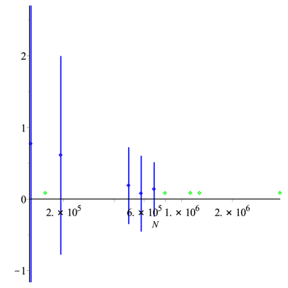
(a)

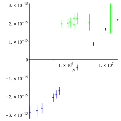
(b)

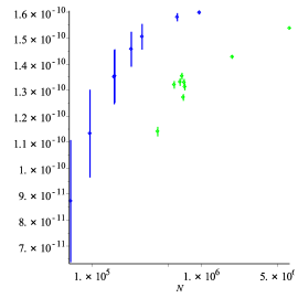
(c)

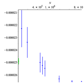
(d)

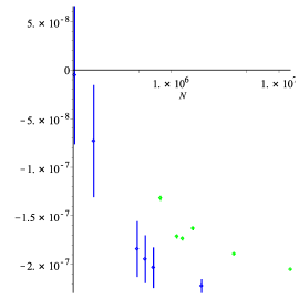
(e)

Figure 7: Several integrals from the tachyon profile calculated with different values of $N$. The error bars are those reported by the Cuhre algorithm. When the Suave algorithm gives results which fit on the same scale they are included as the green data.

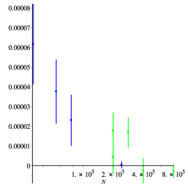
(a)

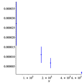
(b)

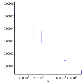
(c)

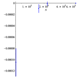
(d)

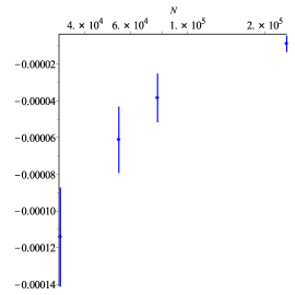
(e)

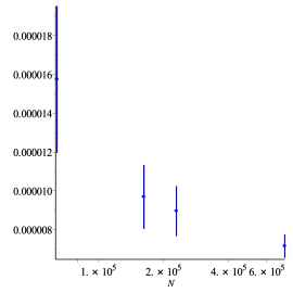
(f)

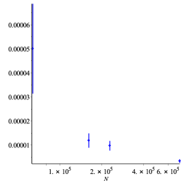
(g)

Figure 8: Several integrals from the consistency checks calculated with different value of $N$. The error bars are those reported by the Cuhre algorithm. When the Suave algorithm gives results which fit on the same scale they are included as the green data.

The first two plots represent the parts of the tachyon profile for which we used the Suave results. In figure 7a the problem is not that the results are inconsistent, but that the errors are so large that the results are meaningless. It looks likely that as $N$ is increased the results will continue to converge to something quite close to the Suave result. For the other integral, figure 7b shows that as $N$ is made extremely large we finally find something like the much more consistent Suave results. The slope, however, does not yet appear to be significantly slowing down, so we cannot be sure that it is convergent. The rest of the plots in figures 7c-7e show the other integrals that contribute to the tachyon profile and have more than a $2\sigma$ variation between points. They all show signs that once $N$ is sufficiently large they converge quite well. Only for smaller $N$ do the error estimates appear to be insufficient.

Moving on to integrals which contribute to consistency checks, in figure 8 we see that the majority are fine. Only 8c does not appear to converge. As with the examples shown in figure 7, this may well be linear until some critical $N$ where it begins to converge. In addition, while only the quantities composed of small sums of these integrals are supposed to vanish, in many cases each of the integrals will vanish independently. These seven examples all become closer to vanishing as $N$ is increased, and only 8f is not getting very close to zero. Convergence of these results does not appear to be very much of an issue, and I expect that if we continued to increase $N$ by another factor of ten they would all continue to approach zero.

3.2 Roundoff errors

Each integrand may contain a number of terms which are divergent either on the boundary of the region, $t_{i}\in\{a,b\}$, or on a diagonal, $t_{i}=t_{j}$. While the renormalization is designed specifically so that these divergences will cancel, individual terms evaluated near these regions can be very large. Because we are limited to the double precision floating point datatype, each term has a relative precision of approximately $10^{-16}$. Any time an individual term is more than $10^{16}$ times the theoretical value of the integrand evaluated at the same point, the machine uncertainty coming from that term can dominate the result. We would hope that since this only happens for a small subset of the points sampled the effect will be negligible as the number of points increases, but this is not the case. If we take a random sample of $N$ points, as is done for Monte Carlo integration, we would expect the closest point to a given boundary (or other codimension 1 subspace) to be $\sim\frac{1}{N}$ away. Individual terms, however, often have a $\frac{1}{t^{2}}$ divergence from the OPE of the marginal operator, which would lead to $\sim N^{2}$ divergence for the closest point. This grows faster than the denominator, $N$, so the roundoff error in the resulting integral should increase linearly with the number of points. The deterministic case is actually worse because some points are intentionally chosen near or even right on the boundary. To combat this, whenever a sample point is close to a boundary or a diagonal, we can replace it with a nearby point giving a decent approximation to the integrand. The integrand function is effectively replaced by one where the value is held constant on small strips. While this means that a perfect integration with no uncertainty would give an incorrect result, the errors introduced this way are less problematic than the roundoff errors when we sample many points without any regulation.

When we discussed the differences between the big $G$ and little $g$ renormalization schemes, we saw that the lack of a regulator was an advantage of the little $g$ scheme. Here we have introduced another regulator, so we naturally ask why this is not a problem. The regulator in the big $G$ scheme was required by the theory in that scheme, and we wanted the limit as it approached zero. This regulator is to prevent roundoff error, which is the unavoidable result of using a floating point datatype. Since we are regulating the integration region anyway, we might ask why (aside from issues regarding finiteness at higher orders) we did not use the big $G$ scheme. By using the little $g$ scheme, the integrand is independent of the regulator, which simplifies the integration process. There is not a different integrand for each value of the regulator, and instead of a limit, we only use a small value of the regulator, namely $3\cdot 10^{-4}$, for which the integrands always evaluate with negligible errors. The choice of regulator for these roundoff errors is arbitrary, but we can estimate the error we have introduced by using the same regulator to replace the value of the integrand with zero near boundaries and diagonals. Fortunately, the differences are minor compared with the statistical errors which are accounted for by the algorithms’ reported uncertainties.

3.3 Consistency checks

Since the programs to construct wedge states with insertions and produce and evaluate integrals corresponding to the tachyon profile are quite complicated, it is worth using them to evaluate some known quantities. We will see that the numerical integration process gives results which are consistent with expectations the majority of the time, despite the presence of counterterms and the uncertain nature of numerical integration. An obvious choice for a quantity which we know is the equation of motion, which should vanish. The equation of motion, however, has ghost number two, which means that its expectation value by itself will trivially vanish because the ghosts are not saturated. In order to test that $Q_{B}\Psi+\Psi*\Psi$ vanishes we test that its overlaps with various other string fields all vanish. Because the equation of motion is stronger than just requiring that the equation of motion annihilates all states and actually tells us that it should vanish exactly, as long as the string field is constructed properly these correlation functions should work out to zero whether they themselves were computed correctly or not. In order to test that a non-trivial result also gives the correct answer, we look to the action. Because this is an exactly marginal solution, we expect the energy to vanish, and because the energy is proportional to the action, the action should vanish as well. The action has ghost number three and does not need any additional test states inserted. That this also vanishes is our first strong test that non-trivial expectation values are computed successfully. A summary of these test calculations and their results using the deterministic algorithms is found in tables 6 and 7 at the end of this section, and all of them are expected to vanish. The majority of the results are consistent with zero, but a few exceptions require detailed examination. These six examples are in table 4, which restates their values using the deterministic algorithms and then includes the corresponding results with Monte Carlo calculations and with deterministic calculations using a vanishing integrand near borders and diagonals where cancelling singularities may occur.

The values in tables 6 and 7 all use a border with width $\epsilon=3\cdot 10^{-4}$. When the integrand is sampled within $\epsilon$ of a boundary or a diagonal, the closest point on the edge of this strip is used instead. In the last column of table 4, when the integrand was sampled at points within these strips, zero was returned instead. The difference between these results gives an estimate of how important the regulated region is to the final result of the integral, and we can see that in most cases it is small compared to the error estimates.

Quantity	Cuhre/QAG	Suave	Cuhre/QAG with 0
$\langle ce^{X^{(0)}},\text{EOM}^{(3)}\rangle$	$(-6.1\pm 0.6)\cdot 10^{-11}$	$(4.1\pm 0.4)\cdot 10^{-4}$	$(-6.1\pm 0.6)\cdot 10^{-11}$
$\langle\Psi^{(1)},\text{EOM}^{(3)}\rangle$	$(-8.5\pm 0.8)\cdot 10^{-11}$	$(6.1\pm 0.7)\cdot 10^{-4}$	$(-8.5\pm 0.8)\cdot 10^{-11}$
$\langle\Psi,Q_{B}\Psi\rangle^{(4)}$	$(-8.7\pm 1.2)\cdot 10^{-10}$	$(-1.5\pm 1.3)\cdot 10^{-2}$	$(-8.7\pm 1.2)\cdot 10^{-10}$
$\frac{\partial}{\partial C^{L}}\langle ce^{3X^{0}},\text{EOM}^{(5)}\rangle$	$(6.2\pm 2.1)\cdot 10^{-5}$	$(-0.3\pm 1.1)\cdot 10^{-6}$	$(-0.4\pm 1.3)\cdot 10^{-4}$
$\frac{\partial}{\partial C_{0}}\langle c,\text{EOM}^{(6)}\rangle$	$(-2.2\pm 0.5)\cdot 10^{-4}$	$(8.7\pm 7.8)\cdot 10^{-4}$	$(0.1\pm 2.1)\cdot 10^{-2}$
$\frac{\partial}{\partial C_{1}}\langle\Psi^{(3)},\text{EOM}^{(3)}\rangle$	$(-3.0\pm 0.2)\cdot 10^{-8}$	$(-5.1\pm 0.7)\cdot 10^{-4}$	$(0.8\pm 1.7)\cdot 10^{-3}$

Table 4: Numerical results for consistency checks which require further analysis. Among the results which are expected to vanish, these six have deterministic results which do not. They are given using the standard deterministic algorithms Cuhre and QAG, using the adaptive Monte Carlo algorithm Suave, and using the deterministic algorithms with the integrand replaced with 0 on the regulated strips near potential singularities instead of using the value of the integrand at a safe nearby point.

Algorithm	Quantity	Result	Dimensions and Sample Sizes
Cuhre	$\frac{\partial}{\partial C^{L}}\langle ce^{3X^{0}},\text{EOM}^{(5)}\rangle$	$(6.2\pm 2.1)\cdot 10^{-5}$	2	16055	3	32131
		$(3.7\pm 1.6)\cdot 10^{-5}$		18005		54229
		$(2.3\pm 1.3)\cdot 10^{-5}$		25545		76581
		$(0.2\pm 1.7)\cdot 10^{-6}$		81055		243205
Cuhre	$\frac{\partial}{\partial C_{0}}\langle c,\text{EOM}^{(6)}\rangle$	$(-2.2\pm 0.5)\cdot 10^{-4}$	3	32131	4	64107
		$(-7.1\pm 2.6)\cdot 10^{-5}$		54229		162027
		$(-4.0\pm 1.7)\cdot 10^{-5}$		76581		229347
		$(-9.1\pm 5.2)\cdot 10^{-6}$		243205		729045
Cuhre	$\frac{\partial}{\partial C_{1}}\langle\Psi^{(3)},\text{EOM}^{(3)}\rangle$	$(-2.96\pm 0.19)\cdot 10^{-8}$	3	32131
		$(-2.99\pm 0.13)\cdot 10^{-8}$		54229
		$(-2.99\pm 0.11)\cdot 10^{-8}$		76581
		$(-3.01\pm 0.06)\cdot 10^{-8}$		243205

Table 5: Three of the consistency checks in table 4 are shown with different sample sizes. The first two are computed as the sum of two integrals with different dimensions, while the third is a single integral. We expect to see results which tend towards zero as the sample size is increased.

Looking at table 4, the first two quantities, $\langle ce^{X^{(0)}},\text{EOM}^{(3)}\rangle$ and $\langle\Psi^{(1)},\text{EOM}^{(3)}\rangle$, have very similar behaviours because the second integrand is $\sqrt{2}$ times the first. They are one dimensional integrals, so we can do them analytically and find that the results are exactly zero. The integrands for these two are increasing as they approach each of the boundaries, which would suggest that the discrepancy comes from the regulated region, but the results with 0 inserted near the boundaries are identical. In fact, the QAG algorithm always seems to give identical results with either choice of regulation near the boundaries, suggesting that that it does not pick points too close to the limits of integration. If we redo these integrals requesting much higher accuracy, however, we find results which are less precise but consistent with zero. Perhaps requesting a higher accuracy causes the algorithm to notice the cusp where the regulated strips at the boundary are, and that increases the error estimate. The kinetic energy at fourth order is a peculiar case of rounding errors, and it was already discussed in the context of convergence. None of the integration algorithms is correct all of the time, and we should not expect them to be, but QAG is problematic because it gives less control over the sample size and does not report the total number of points it uses. We cannot show these results with different sample sizes, as we do for other quantities of interest. Because these are one-dimensional integrals, however, we can expect that the majority of them will be computed very accurately.

For the other three quantities, the integrals are multidimensional so we can evaluate them using the Cuhre algorithm with several different sample sizes and see if they become closer to zero. This is shown in table 5. The first two of these both have error estimates that decrease as the sample size is increased, and values that decrease even faster. For the first, we see agreement once the sample size is large enough, and for the second we can suspect that the result will continue to tend towards zero. The most important integrals in these two quantities were shown in figures 8a and 8d respectively, where we can see the convergence to 0 as $N$ is increased. In the case of the final quantity, however, the result clearly does not vanish. If we change the thickness of the regulating border, however, it causes a significant fluctuation, and for extremely thin borders both the result and the uncertainty become much larger. This suggests that it is a genuine case of the border region having a significant impact. Unfortunately, the only way to resolve this issue would be to use higher precision floating point datatypes.

$\langle c,\text{EOM}^{(2)}\rangle$	$0$
$\langle ce^{2X^{0}},\text{EOM}^{(2)}\rangle$	$0$
$\langle ce^{X^{0}},\text{EOM}^{(3)}\rangle$	$-(6.1\pm 0.6)\cdot 10^{-11}$
$\langle ce^{3X^{0}},\text{EOM}^{(3)}\rangle$	$0\pm 1.1\cdot 10^{-16}$
$\langle c,\text{EOM}^{(4)}\rangle$	$-(0.6\pm 1.9)\cdot 10^{-6}-(0.8\pm 1.3)\cdot 10^{-6}C^{L}$
$\langle ce^{2X^{0}},\text{EOM}^{(4)}\rangle$	$(1.7\pm 2.5)\cdot 10^{-6}+(9.2\pm 9.7)\cdot 10^{-7}C^{L}$
$\langle ce^{4X^{0}},\text{EOM}^{(4)}\rangle$	$(2.8\pm 8.7)\cdot 10^{-11}$
$\langle ce^{X^{0}},\text{EOM}^{(5)}\rangle$	$(1.8\pm 2.5)\cdot 10^{-5}-(1.3\pm 1.8)\cdot 10^{-5}C^{L}-(0.2\pm 3.2)\cdot 10^{-4}(C^{L})^{2}+(2.1\pm 2.0)\cdot 10^{-5}C_{1}+(0.6\pm 2.3)\cdot 10^{-5}C_{0}$
$\langle ce^{3X^{0}},\text{EOM}^{(5)}\rangle$	$(0.2\pm 2.3)\cdot 10^{-5}+(6.2\pm 2.1)\cdot 10^{-5}C^{L}-(0.3\pm 2.7)\cdot 10^{-5}C_{1}-(0.7\pm 6.6)\cdot 10^{-6}C_{0}$
$\langle ce^{5X^{0}},\text{EOM}^{(5)}\rangle$	$(0.2\pm 3.8)\cdot 10^{-11}$
$\langle c,\text{EOM}^{(6)}\rangle$	$-(0.8\pm 2.0)\cdot 10^{-3}+(0.7\pm 1.9)\cdot 10^{-4}C^{L}-(1.6\pm 5.4)\cdot 10^{-5}(C^{L})^{2}-(1.8\pm 2.3)\cdot 10^{-4}C_{1}+(0.2\pm 7.1)\cdot 10^{-3}C^{L}C_{1}-(2.2\pm 0.5)\cdot 10^{-4}C_{0}+(1.9\pm 6.5)\cdot 10^{-5}C_{0}C^{L}$
$\langle ce^{2X^{0}},\text{EOM}^{(6)}\rangle$	$-(0.1\pm 1.3)\cdot 10^{-3}+(0.7\pm 3.7)\cdot 10^{-4}C^{L}+(0.2\pm 1.9)\cdot 10^{-3}(C^{L})^{2}+(0.1\pm 2.1)\cdot 10^{-3}C_{1}+(0\pm 1.5\cdot 10^{-2})C^{L}C_{1}+(0.9\pm 5.1)\cdot 10^{-4}C_{0}-(0.1\pm 2.9)\cdot 10^{-3}C^{L}C_{0}$
$\langle ce^{4X^{0}},\text{EOM}^{(6)}\rangle$	$0\pm 1.1\cdot 10^{-5}+(1.4\pm 1.0)\cdot 10^{-6}C^{L}-(0.2\pm 5.9)\cdot 10^{-6}C_{1}+(0.4\pm 8.9)\cdot 10^{-7}C_{0}$
$\langle ce^{6X^{0}},\text{EOM}^{(6)}\rangle$	$-(0.6\pm 1.3)\cdot 10^{-14}$
$\langle\Psi^{(1)},\text{EOM}^{(2)}\rangle$	$0$
$\langle\Psi^{(2)},\text{EOM}^{(2)}\rangle$	$0$
$\langle\Psi^{(3)},\text{EOM}^{(2)}\rangle$	$0$
$\langle\Psi^{(4)},\text{EOM}^{(2)}\rangle$	$0$
$\langle\Psi^{(5)},\text{EOM}^{(2)}\rangle$	$0$
$\langle\Psi^{(1)},\text{EOM}^{(3)}\rangle$	$-(8.5\pm 0.8)\cdot 10^{-11}$
$\langle\Psi^{(2)},\text{EOM}^{(3)}\rangle$	$0$
$\langle\Psi^{(3)},\text{EOM}^{(3)}\rangle$	$-(0.5\pm 1.3)\cdot 10^{-5}-(0.1\pm 3.4)\cdot 10^{-6}C^{L}-(3.0\pm 0.2)\cdot 10^{-8}C_{1}$
$\langle\Psi^{(4)},\text{EOM}^{(3)}\rangle$	$0$
$\langle\Psi^{(1)},\text{EOM}^{(4)}\rangle$	$0$
$\langle\Psi^{(2)},\text{EOM}^{(4)}\rangle$	$-(0.3\pm 2.4)\cdot 10^{-3}+(2.3\pm 5.2)\cdot 10^{-5}C^{L}-(0.2\pm 1.8)\cdot 10^{-5}(C^{L})^{2}$
$\langle\Psi^{(3)},\text{EOM}^{(4)}\rangle$	$0$
$\langle\Psi^{(1)},\text{EOM}^{(5)}\rangle$	$(2.4\pm 3.9)\cdot 10^{-5}-(1.9\pm 2.5)\cdot 10^{-5}C^{L}-(0.3\pm 4.5)\cdot 10^{-4}(C^{L})^{2}+(3.0\pm 2.8)\cdot 10^{-5}C_{1}+(0.8\pm 3.2)\cdot 10^{-5}C_{0}$
$\langle\Psi^{(2)},\text{EOM}^{(5)}\rangle$	$0$
$\langle\Psi^{(1)},\text{EOM}^{(6)}\rangle$	$0$

Table 6: Deterministic tests of the equation of motion for the rolling tachyon. Superscripts represent the order in $\lambda$ of each quantity. Cuhre/QAG results shown.

$\langle\Psi,Q_{B}\Psi\rangle^{(2)}$	$0$
$\langle\Psi,\Psi*\Psi\rangle^{(2)}$	$0$
$\langle\Psi,Q_{B}\Psi\rangle^{(3)}$	$0$
$\langle\Psi,\Psi*\Psi\rangle^{(3)}$	$0$
$\langle\Psi,Q_{B}\Psi\rangle^{(4)}$	$-(8.7\pm 1.2)\cdot 10^{-10}+(0\pm 4.2\cdot 10^{-14})C^{L}$
$\langle\Psi,\Psi*\Psi\rangle^{(4)}$	$0$
$\langle\Psi,Q_{B}\Psi\rangle^{(5)}$	$0$
$\langle\Psi,\Psi*\Psi\rangle^{(5)}$	$0$
$\langle\Psi,Q_{B}\Psi\rangle^{(6)}$	$(0.02\pm 0.30)+(0\pm 3.5\cdot 10^{-2})C^{L}+(0\pm 0.11)(C^{L})^{2}+(0.5\pm 9.6)\cdot 10^{-13}(C^{L})^{3}+(0\pm 6.7\cdot 10^{-2})C_{1}-(0.1\pm 2.3)\cdot 10^{-13}C^{L}C_{1}+(0\pm 1.1\cdot 10^{-2})C_{0}+(0.1\pm 1.5)\cdot 10^{-14}C^{L}C_{0}$
$\langle\Psi,\Psi*\Psi\rangle^{(6)}$	$0$

Table 7: Deterministic evaluation of the action for the rolling tachyon. Kinetic and cubic terms are found separately as a consistency check. Superscripts represent the order in $\lambda$. Cuhre/QAG results shown.

References

- [1] M. Kiermaier and Y. Okawa, Exact marginality in open string field theory: a general framework, JHEP 11 (2009) 041, [arXiv:0707.4472].
- [2] J. L. Karczmarek and M. Longton, Renormalization schemes for SFT solutions, JHEP 1504 (2015) 007, [arXiv:1412.3466].
- [3] E. Coletti, I. Sigalov, and W. Taylor, Taming the tachyon in cubic string field theory, JHEP 0508 (2005) 104, [hep-th/0505031].
- [4] T. Erler, Level truncation and rolling the tachyon in the lightcone basis for open string field theory, hep-th/0409179.
- [5] M. Kiermaier, Y. Okawa, L. Rastelli, and B. Zwiebach, Analytic solutions for marginal deformations in open string field theory, JHEP 01 (2008) 028, [hep-th/0701249].
- [6] M. Schnabl, Comments on marginal deformations in open string field theory, Phys. Lett. B654 (2007) 194–199, [hep-th/0701248].
- [7] M. Kiermaier, Y. Okawa, and P. Soler, Solutions from boundary condition changing operators in open string field theory, JHEP 03 (2011) 122, [arXiv:1009.6185].
- [8] I. Ellwood, Rolling to the tachyon vacuum in string field theory, JHEP 0712 (2007) 028, [arXiv:0705.0013].
- [9] E. Fuchs, M. Kroyter, and R. Potting, Marginal deformations in string field theory, JHEP 0709 (2007) 101, [arXiv:0704.2222].
- [10] C. Maccaferri, A simple solution for marginal deformations in open string field theory, arXiv:1402.3546.
- [11] T. Erler and C. Maccaferri, String Field Theory Solution for Any Open String Background, JHEP 1410 (2014) 029, [arXiv:1406.3021].
- [12] T. Hahn, CUBA: A Library for multidimensional numerical integration, Comput.Phys.Commun. 168 (2005) 78–95, [hep-ph/0404043].