HST/COS Detection of the Spectrum of the Subdwarf Companion of KOI-81

Abstract

KOI-81 is a totally eclipsing binary discovered by the Kepler mission that consists of a rapidly rotating B-type star and a small, hot companion. The system was forged through large scale mass transfer that stripped the mass donor of its envelope and spun up the mass gainer star. We present an analysis of UV spectra of KOI-81 that were obtained with the Cosmic Origins Spectrograph on the Hubble Space Telescope that reveal for the first time the spectral features of the faint, hot companion. We present a double-lined spectroscopic orbit for the system that yields mass estimates of $2.92M_{\odot}$ and $0.19M_{\odot}$ for the B-star and hot subdwarf, respectively. We used a Doppler tomography algorithm to reconstruct the UV spectra of the components, and a comparison of the reconstructed and model spectra yields effective temperatures of 12 kK and 19 – 27 kK for the B-star and hot companion, respectively. The B-star is pulsating, and we identified a number of peaks in the Fourier transform of the light curve, including one that may indicate an equatorial rotation period of 11.5 hours. The B-star has an equatorial velocity that is $74\%$ of the critical velocity where centrifugal and gravitational accelerations balance at the equator, and we fit the transit light curve by calculating a rotationally distorted model for the photosphere of the B-star.

1 Introduction

The NASA Kepler mission of precise and long time span photometry has led to many surprising discoveries. Among the initial set of remarkable targets, Rowe et al. (2010) reported on observations of two transiting systems dubbed KOI-74 ($P=5.2$ d) and KOI-81 ($P=23.9$ d) that display light curves with minima that were deeper during occultation than during transit, implying that the planetary size companions are hotter than their A- or B-type host stars. Rowe et al. (2010) proposed that these companions were actually very low mass white dwarf (WD) stars, the remnants of more massive progenitors in an interacting binary. The light curves of both systems were further analyzed by van Kerkwijk et al. (2010) who found that both appear more luminous during orbital phases of the bright star approach due to relativistic Doppler boosting (“beaming binaries”; Zucker et al. 2007). Van Kerkwijk et al. used the radial velocity semiamplitude implied by Doppler boosting to estimate that the white dwarf stars had masses of $\approx 0.2-0.3M_{\odot}$.

The Kepler observations eventually led to the discovery of other similar eclipsing binary systems. Carter et al. (2011) found that KIC 10657664 consists of a hot WD orbiting an A-type star ($P=3.3$ d), and Breton et al. (2012) discovered a WD and F-star binary system, KOI-1224 ($P=2.7$ d). Two more systems orbiting A-type stars were recently discovered by Rappaport et al. (2015), KIC 9164561 ($P=1.3$ d) and KIC 10727668 ($P=2.3$ d). Maxted et al. (2011, 2014) reported on the detection of 18 similar short-period systems ($P=0.7-2.2$ d) in photometric time series from the ground-based Wide Angle Search for Planets survey program. Photometric detection of longer period systems is less probable because the orbital inclination must be extremely close to $90^{\circ}$ for transits to occur. However, longer period systems can be found through extensive, time series, radial velocity measurements from spectroscopy. For example, Gies et al. (2008) used radial velocity measurements to show that the nearby star Regulus is a spectroscopic binary ($P=40.1$ d) consisting of a B-star with a probable WD companion. These hot companions of main sequence stars are probably related to the subdwarf companions of rapidly rotating Be stars that are detected through ultraviolet spectroscopy (Peters et al. 2013).

Close binaries are common among intermediate mass stars, and many of these will experience large scale mass transfer (Rappaport et al. 2009; van Kerkwijk et al. 2010; Di Stefano 2011; Clausen et al. 2012). As the initially more massive star grows in radius, this donor star will begin Roche lobe overflow (RLOF) and transfer mass and angular momentum to the companion (the mass gainer). The orbit will shrink until the masses are equal, and if contact can be avoided, then additional mass transfer will cause an expansion of the orbit that ceases once the donor has lost its envelope. The resulting system will consist of a stripped-down and hot donor star in orbit around a rapidly rotating and more massive gainer star.

Detecting binaries in this stage of evolution is difficult because the small donor stars are relatively faint and lost in the glare of the brighter companions. Furthermore, the donors are now low mass objects that create only small reflex orbital motions in the gainer stars, so detection through spectroscopy is challenging. Thus, the Kepler discoveries offer us a remarkable opportunity to investigate the properties of stars that are known examples of this post-mass transfer state. The hot companions will contribute a larger fraction of the total flux at shorter wavelengths, so a direct search for the flux and spectral features associated with the hot companion is best done in the ultraviolet. Indeed, it was through UV spectroscopy from the International Ultraviolet Explorer satellite (Thaller et al. 1995) and from the Hubble Space Telescope (Gies et al. 1998) that the hot subdwarf companion of the Be star $\phi$ Per was first detected.

Here we report on an UV spectroscopic investigation of KOI-81 (KIC 8823868; TYC 3556-3094-1; 2MASS J19350857+4501065) made possible with the HST Cosmic Origins Spectrograph (COS) that has revealed the spectral features of the hot companion for the first time. We describe the COS observations and supporting ground-based spectroscopy in §2. We present radial velocity measurements and a double-lined orbital solution in §3 to obtain mass estimates. We then use the derived radial velocity curves to perform a Doppler tomographic reconstruction of the component spectra, and we compare the reconstructed spectra to model spectra to derive effective temperatures and projected rotational velocities (§4). The Kepler light curve outside eclipses shows evidence of pulsational and rotational frequency signals that we discuss in §5. The transit light curve is analyzed in §6 using a model for the rotationally distorted B-star. We summarize and consider some consequences of the results in §7.

2 Spectroscopic Observations

The Cosmic Origins Spectrograph (COS) is a high dispersion instrument designed to record the UV spectra of point sources (Osterman et al. 2011; Green et al. 2012). The HST/COS observations of KOI-81 were obtained over five visits between 2011 June and 2011 October. These were scheduled so that two occurred during each of the quadrature phases near the Doppler shift extrema, and the fifth observation was made during the hot star occultation phase in order to isolate the flux of the B-star alone. The UV spectra were made with the G130M grating to record the spectrum over the range from 1150 to 1450 Å with a spectral resolving power of $R=\lambda/\triangle\lambda=18000$. There are two COS detectors that are separated by a small gap, so the spectra were made at slightly different central wavelengths in order to fill in the missing flux: 1300 Å (four exposures of 447 s), 1309 Å (three exposures of 399 s), and 1318 Å (three exposures of 399 s). This sequence required an allocation of two orbits for each visit. The observations were processed with the standard COS pipeline to create wavelength and flux calibrated spectra as x1d.fits files for each central wavelength arrangement (Massa et al. 2013). These ten sub-exposures were subsequently merged onto a single barycentric wavelength grid using the IDL procedure coadd_x1d.pro (Danforth et al. 2010). We created a list of the sharp interstellar lines in the spectrum, and we cross-correlated each of these spectral regions with those in the average spectrum in order to make small corrections to the wavelength calibration. Then the interstellar lines were removed in each spectrum by linear interpolation across their profiles. Finally, all five spectra were transformed to a uniform grid with a $\log\lambda$ pixel spacing equivalent to a Doppler shift step size of 2.60 km s^-1 over the range from 1150 to 1440 Å. The coadded spectra have a signal-to-noise ratio of S/N = 110 in the central, best exposed parts.

We also obtained three sets of complementary ground-based spectra of KOI-81. The first set consists of 19 high dispersion spectra made with Tillinghast Reflector Echelle Spectrograph (TRES) mounted on the 1.5 m Tillinghast telescope at the Fred Lawrence Whipple Observatory at Mount Hopkins, Arizona. These spectra cover the optical range from 3850 to 9100 Å with a resolving power of $R=\lambda/\triangle\lambda=48000$. The spectra were processed and rectified to intensity versus wavelength using standard procedures (Buchhave et al. 2010), and they are available at the Kepler Community Follow-up Observing Program (CFOP) website. A second set of six moderate resolution spectra were made in 2010 and 2012 with the Kitt Peak National Observatory (KPNO) 4 m Mayall telescope and the Ritchey-Chretien (RC) Focus Spectrograph. These were made with the BL 380 grating (1200 grooves mm^-1) to record the spectrum between 3950 to 4600 Å with a resolving power of $R=6300$. Finally a third set of five, lower resolution, and flux calibrated spectra were obtained in 2010 with the Mayall telescope and RC spectrograph using the KPC-22B grating (632 grooves mm^-1) to cover the region from 3577 to 5058 Å with a resolving power of $R=2500$. This third set is also available at the CFOP website.

3 Radial Velocities and Orbital Elements

Our first goal was to measure the orbital motion of the primary star using the COS UV spectra. Direct inspection of the spectra showed that the main features were very broadened and blended due to large rotational broadening (§4). Consequently, we decided to measure the individual spectrum velocities by cross-correlating them with a spectral template. We formed cross-correlation functions (CCFs) using the hot star occultation phase spectrum (made on HJD 2455775.9626) as the CCF template. The calculation was made using only the regions from 1270 to 1300 Å and from 1314 to 1437 Å (see Fig. 4 below) in order to avoid the low wavelength region where the secondary’s flux becomes larger and to remove the Si II $\lambda\lambda 1260,1264,1304,1309$ features that may be affected by incomplete removal of the interstellar components. The resulting CCFs are extremely broad, and we found the center of each CCF by measuring the wing bisector position by convolving the CCF wings with oppositely signed Gaussian functions (Shafter et al. 1986). We similarly measured the center of the CCF of the hot star occultation phase spectrum with a model spectrum for the B-star (§4) from the UVBLUE library (Rodríguez-Merino et al. 2005), and this offset was added to the relative velocities to transform them to an absolute scale. The resulting radial velocities are collected in Table 1 that lists a leading P or S for primary B-star or secondary hot star (see below), the heliocentric Julian date of mid-observation, the orbital phase based upon the Kepler solution for the time of mid-transit (B-star superior conjunction), the radial velocity, the difference between the radial velocity and the systemic velocity for the specific observation set (see below), the uncertainty $\sigma$, the observed minus calculated ($O-C$) velocity residual from the fit (§4), and the source (HST/COS in this case). Both pairs of quadrature observations were separated in time by only a few hours and are expected to have almost the same orbital velocity, so we used the absolute differences of the measured velocities of these pairs to estimate $\sqrt{2}\sigma$.

We realized at the outset that finding and measuring the spectral lines of the companion would be challenging because of its relative faintness. However, detection is favored at the shorter wavelength part of the UV spectrum because the hotter companion contributes relatively more flux there. An inspection of the spectra in the region with $\lambda<1200$ Å did indeed hint at the presence of a velocity variable, narrow-lined component. We needed to isolate the flux contribution from the bright B-star in this region in order to remove its flux from each spectrum and reveal the secondary’s spectral lines in the flux difference. This was accomplished using the hot star occultation phase spectrum to represent the flux of the B-star alone. This spectrum was smoothed by convolution with a Gaussian function of FHWM = 133 km s^-1 in order to increase the S/N ratio without unduly altering the spectral shape. Then the smoothed version was shifted in velocity according to the predicted orbital motion of the primary star, and a difference spectrum was formed for each of the four quadrature phase observations. Renormalized and averaged versions of these quadrature phase spectra are illustrated in Figure 1, and these show a host of weak and narrow lines that are Doppler shifted as expected for the orbital motion of the hot secondary. The flux scaling for the hot companion is not accurate because of the rudimentary means of the B-star’s flux removal, but it is sufficient to reveal the lines of the hot component so that its radial velocity can be measured. We did so by calculating the CCF of each quadrature spectrum using a hot model spectrum (§4) for the template, and the center of the narrow signal in the resulting CCF was estimated by fitting a parabola to its peak (with uncertainties determined using the method of Zucker 2003). The derived radial velocities of the secondary are listed at bottom of Table 1 in rows with a leading column marked S. No measurement is given for the occultation phase spectrum because the flux of the hot component is totally blocked then (Rowe et al. 2010).

We also measured radial velocities for the primary B-star using the higher resolution, ground-based spectra. The 19 TRES spectra have a S/N that is too low for measurement of the weak and broadened He and metallic lines, but they are sufficient to measure the Doppler shifts in the strong and broad, H Balmer lines. We formed CCFs of each of H$\alpha$, H$\beta$, H$\gamma$, H$\delta$, and H$\epsilon$ with model template spectra from the BLUERED grid (Bertone et al. 2008). The radial velocity was estimated by fitting a parabola to the peak of the CCF for each line. The quality of the measurement varies depending on the position of the feature relative to the echelle blaze function (best for H$\alpha$ and H$\gamma$ which fall close to the blaze maximum), so we formed weights for each of the Balmer lines proportional to the inverse square of the standard deviation of the velocity measurements. We then determined the weighted mean and standard deviation of the mean from the set of five line measurements for each observation, and these are listed in Table 1 (noted by TRES in the final column).

We followed a similar procedure to measure radial velocities for the six KPNO moderate resolution spectra. We calculated CCFs using a model B-star template (from the UVBLUE grid) and including all the lines in the region from 4050 to 4520 Å (dominated by H$\gamma$ and H$\delta$), and we fit a parabola to the CCF peak to estimate radial velocities. These are identified in Table 1 by KPNO in the final column.

We fit orbital elements for each of the primary and secondary velocity sets using the program described by Morbey & Brosterhus (1974). We fixed the orbital period and epoch of mid-transit to those derived by the Kepler project (dated 2014 November 24) that are posted at the CFOP website. Because the transit and occultation light curves have the same duration and are separated by half of the orbital period, we assumed that the orbit is circular. We set the fitting weights to the inverse square of the uncertainties. Because the COS, TRES, and KPNO measurements are derived from differing spectral ranges and instruments, we might expect that there will be systematic differences in the velocities for each set. The upper panel of Figure 2 shows the measured radial velocities from Table 1, using different symbols for each set of spectra, as well as preliminary fits of each set, and there do indeed appear to be constant offsets between the sets. We found independent estimates for the systemic velocity $\gamma_{i}$ of each set by iterating between global (all data) and individual sets of velocities for the orbital fits. This was done by fixing the semiamplitude $K_{1}$ from the global fit to find estimates of $\gamma_{i}$ for solutions to each set. Then a new global fit was made using velocity differences (subtracting the $\gamma_{i}$ value associated with each set) to find a revised $K_{1}$. This procedure converged after a few iterations to the final adopted fit presented in Table 2. The $\gamma_{i}$-corrected velocities (listed under column $V_{r}-\gamma_{i}$ in Table 1) and $2\sigma$ range of the fitted velocity of the primary are shown in the lower panel of Figure 2, and the combined velocity curves of the primary and secondary are illustrated in Figure 3. We also made a fit of the $\gamma_{i}$-corrected velocities of the primary using a Markov Chain Monte Carlo algorithm that led to almost the same result, $K_{1}=6.75^{+0.43}_{-0.44}$ km s^-1. However, we conservatively adopt the somewhat larger uncertainty estimates from the non-linear least squares program in what follows. Van Kerkwijk et al. (2010) estimated $K_{1}\approx 7$ km s^-1 from the Doppler boosting in the light curve of KOI-81, and their result is verified through our direct Doppler shift measurement of $K_{1}=6.7\pm 0.7$ km s^-1.

The orbital inclination is very close to $i=90^{\circ}$. We derive a value from the transit light curve (§6) of $i=88\fdg 97\pm 0\fdg 04$, which is intermediate between the estimates from Rowe et al. (2010) of $i=88\fdg 2\pm 0\fdg 3$ and from the Kepler project posted at CFOP of $i=89\fdg 95$. Thus, we can use our estimate to derive the physical masses from the $M_{1}\sin^{3}i$, $M_{2}\sin^{3}i$ products, and these are given in Table 3. Furthermore, the average density $\rho$ of the B-star can be directly estimated from the transit light curve (provided the star is spherical; see §6), and the Kepler project finds $\rho=0.280\pm 0.005$ g cm^-3 for KOI-81 (reported at the CFOP website). We used this value together with the mass estimate $M_{1}$ to arrive at the radius $R_{1}$ reported in Table 3. Finally, the CFOP website gives the ratio of the radii derived from the transit light curve, $R_{2}/R_{1}=0.03725\pm 0.00026$, and we used this ratio to find $R_{2}$ (Table 3). Table 3 also presents the gravitational acceleration $\log g$ derived from the mass and radius information. We must examine the spectrum of the system to derive the remaining stellar parameters.

4 Tomographic Reconstruction of the UV Spectra

We used a Doppler tomography algorithm (Bagnuolo et al. 1994) to extract the individual UV spectra of the primary and secondary stars. This is an iterative scheme that uses estimates of the orbital Doppler shifts of each component and their flux ratio to derive reconstructed spectra for both stars. We initially assumed featureless continua as the starting approximation for the spectra of both stars, but after comparison with model spectra, we ran the algorithm again using the models as starting values, and this choice helped to limit the continuum wander in the resulting spectral reconstructions. We present in Figures 4 and 5 the reconstructed UV spectra derived from the four COS spectra obtained at the quadrature phases. Figure 4 also shows the excellent agreement between the reconstructed spectrum of the primary and the hot star occultation phase spectrum that represents the flux of the primary alone. Figures 4 and 5 indicate some of the principal lines as well as the locations of the interstellar lines, where their removal by interpolation may have interfered with the accurate reconstruction of the spectra. All the spectra in Figures 4 and 5 are smoothed by convolution with a boxcar function of width 133 km s^-1 in order to reduce the noise and facilitate intercomparison of the line features.

We compared the reconstructed spectra with model spectra from the UVBLUE grid of high resolution spectra calculated by Rodríguez-Merino et al. (2005) that are based upon the ATLAS9 model atmosphere code and SYNTHE radiative transfer code developed by R. L. Kurucz. We used their solar metallicity models that incorporate a microturbulent velocity of 2 km s^-1. We made simple bilinear interpolations of flux in the $(T_{\rm eff},\log g)$ plane to derive the model spectra. We adopted $\log g_{1}=4.13$ for the primary (Table 3), but set $\log g_{2}=5.0$ for the secondary because this value is the largest available in the UVBLUE grid. The model spectra were rebinned onto the observed wavelength grid and then convolved with the instrumental broadening function (from the COS line spread function for a central wavelength of 1300 Å) and with a rotational broadening function (using linear limb darkening coefficients from Wade & Rucinski 1985).

We first compared the reconstructed and model spectra to estimate the projected rotational velocity $V\sin i$ of each star. This was done by forming a $\chi^{2}$ goodness-of-fit statistic between the observed and model spectra over a test grid of $V\sin i$ values, and then finding the $V\sin i$ corresponding to the minimum $\chi^{2}$. This was repeated for a series of wavelength regions that contained well defined absorption lines or line blends, and the mean and standard deviation of the derived $V\sin i$ for the primary is presented in Table 3. The primary B-star is indeed a very rapidly rotating star, a property noted first by van Kerkwijk et al. (2010). The lines of the hot secondary companion, on the other hand, appear very sharp and any rotational broadening is unresolved in the COS spectra, so we present only an upper limit in Table 3.

Next we needed to adjust the model spectra for the variable interstellar extinction across the COS wavelength band. We derived the interstellar reddening by comparing the available observed fluxes with a model flux distribution for the binary transformed using the extinction law presented by Fitzpatrick (1999). The observed fluxes are shown in a spectral energy distribution plot in Figure 6. These include rebinned COS measurements, a GALEX NUV measurement, rebinned KPNO low dispersion spectrophotometry, and 2MASS and WISE photometric fluxes. The model fluxes were a sum of Kurucz models for the primary and secondary that were attenuated according to the extinction law for a ratio of total-to-selective extinction of $R=3.1$. The fit shown in Figure 6 was made with a reddening of $E(B-V)=0.169\pm 0.008$ mag and a limb darkened angular diameter of the primary of $\theta=0.0182\pm 0.0005$ milliarcsec. The former agrees with prior estimates ($E(B-V)=0.175$ and 0.193 mag in the Kepler Input Catalog and the GALEX Catalog, respectively), and the latter indicates a distance of 1.25 kpc (using $R_{1}/R_{\odot}$ from Table 3). The extinction in the COS band was calculated for the derived value of $E(B-V)$, and each model was multiplied by this extinction curve to account for the greater interstellar attenuation at lower wavelength.

With the gravity, projected rotational velocity, and interstellar extinction set, we then calculated model spectra over a grid of effective temperature and determined a $\chi^{2}$ goodness-of-fit as a function of $T_{\rm eff}$. The best fit temperatures and their estimated uncertainties from this comparison of the reconstructed and model spectra are listed in Table 3. These uncertainties do not account for possible differences from the assumed microturbulent velocity and abundance. Nevertheless, these models offer a framework to interpret the appearance of the UV spectra.

Figure 4 shows the derived model spectrum offset above the reconstructed spectrum of the primary star. The overall agreement is very good in both the appearance of the lines and line blends. The C II $\lambda\lambda 1335,1336$ feature is weaker than predicted, but this may result from our means of removal of interstellar line components in this feature. The flux in the optical wavelength range is totally dominated by the light from the B-star primary (§6), so we did not attempt Doppler tomography reconstructions of the optical spectrum. However, we show in Figure 7 two optical lines of special interest. The most temperature sensitive feature in the optical spectrum at $T_{\rm eff}\approx 10$ kK is the Ca II $\lambda 3933$ K line that grows rapidly in strength with decreasing temperature (Gray & Corbally 2009). The average TRES spectrum of this feature is shown in Figure 7 (left) together with model spectra for $T_{\rm eff}=11.7$ kK and 10.6 kK, and a comparison with the observed K-line suggests that the effective temperature may be somewhat lower than that derived from the ultraviolet spectrum (but still within the uncertainties). On the other hand, the difference may result from gravity darkening in the rapidly rotating B-star that creates a cooler equatorial region (§6) that would promote the appearance of lines favored in cooler atmospheres. Figure 7 also illustrates the average observed and model profiles of the gravity sensitive H$\gamma$ line (right), and the observed profile has a shape that is approximately consistent with predictions for the adopted gravity of the primary.

The reconstructed secondary spectrum shown in Figure 5 is quite noisy because this component is relatively faint (see below), but there is satisfactory agreement between the reconstructed and model spectra in the vicinity of some features. For example, the reconstructed and model spectra of the secondary appear similar in the lines of C III $\lambda 1176$, Si II $\lambda\lambda 1193,1194$, Si III $\lambda\lambda 1295,1297,1299$, and Si IV $\lambda\lambda 1394,1403$. The latter are only seen in the spectrum of the hotter secondary. However, the agreement is less satisfactory in the regions where interstellar lines were removed (near 1229, 1251, 1303, 1335, and 1347 Å). The model spectra were formed using UVBLUE models with $\log g=5.0$, the largest value in the grid, which is smaller than the estimated gravity, $\log g=5.8$. This has two important consequences. First, the model Ly$\alpha$ line is narrower than observed because the linear Stark broadening associated with the lower gravity model is insufficient to match the observed broadening. Second, the effective temperature estimation is based upon the relative strengths of transitions corresponding to different ionization states, and according to the Saha equation, line formation in a denser medium (at higher gravity) will shift the ionization balance to less ionized states. Consequently, a good fit of the spectrum would also be possible with a higher gravity and higher temperature model, so our derived effective temperature should be regarded as a lower limit. We also show in Figure 5 an example spectrum of the B-subdwarf CPD$-64^{\circ}481$ that was made with the Space Telescope Imaging Spectrograph and E140H grating. O’Toole & Heber (2006) used this and other spectra to estimate $T_{\rm eff}=27.5$ kK and $\log g=5.6$, a value of gravity that is closer to that of the secondary in KOI-81. Comparing these similar gravity stellar spectra, we see that transitions of Si II are almost absent in the spectrum of CPD$-64^{\circ}481$, whereas they are quite strong in the spectrum of the KOI-81 secondary, so the KOI-81 secondary must be cooler than CPD$-64^{\circ}481$. Thus, we can place lower and upper limits on the effective temperature of the secondary of $19<T_{\rm eff}<27$ kK.

All the spectra in Figures 4 and 5 were normalized in flux by dividing by the mean flux over the range between 1340 and 1400 Å. We set the monochromatic flux ratio from this normalization to $F_{2}(1370)/F_{1}(1370)=0.05\pm 0.02$ based upon a comparison of the line depths in the reconstructed and model spectra of the secondary. This comparison was made using relative line depths in the vicinity of the lines that matched reasonably well, because there is too much wander in the continuum of the reconstructed spectrum of the secondary for a reliable global fit. We caution that the model line depths are sensitive to the adopted values of temperature, gravity, and especially microturbulence, so the flux ratio may need revision if different assumptions are made.

5 Non-orbital Frequencies in the Light Curve

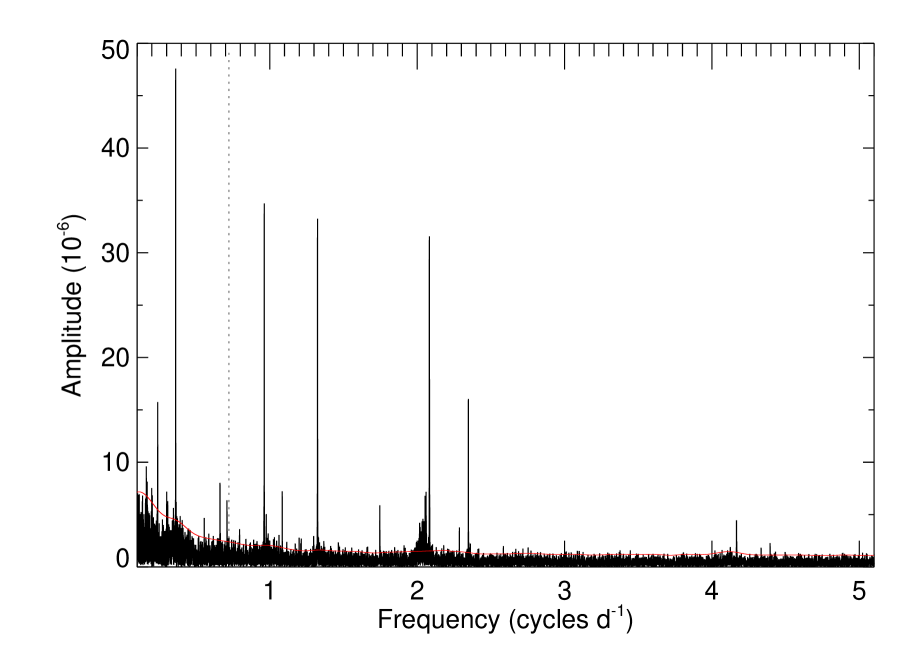
Figure 8: The Fourier amplitude spectrum of Kepler short cadence photometry after prewhitening the dominant peak at $0.72297$ d^-1 indicated by the dotted line. The empirical noise level is indicated by the red solid line.

Both Rowe et al. (2010) and van Kerkwijk et al. (2010) noted that the light curve of KOI-81 shows evidence of pulsations, and it is interesting to consider the pulsational frequencies and their relation to the rotational frequency of the B-star primary. We calculated the Fourier transform amplitude of the detrended, long cadence Kepler observations from quarters 0 to 17 using the package Period$04$ (Lenz & Breger 2005). The portions of the light curve covering the transit and occultation of the secondary were removed from the time series in order to focus on non-orbital timescales of variation. We adopted an empirical noise level by smoothing the envelope of the residual spectrum after prewhitening all significant frequencies with $S/N>3$ (except for the broad rotational feature; see below). The uncertainties were calculated following Kallinger et al. (2008). The Fourier spectrum is dominated by a very strong signal with a frequency of $f_{1}=0.722974$ cycles d^-1 (period of 1.38318 d), so we removed this signal by pre-whitening to uncover the remaining periodic signals that are plotted in Figure 8. There are a number of strong signals that appear well above the noise level, and the frequencies, amplitudes, sinusoidal phases (relative to the epoch of central transit), and peak signal-to-noise ratio are listed in Table 4. The final column of Table 4 lists several numerical relations among these frequencies, and identifies one frequency $f_{12}$ that corresponds to the ellipsoidal (tidal) variation with half the orbital period (discussed by van Kerkwijk et al. 2010).

The dominant periodicity (1.38 d) is unrelated to the orbital period, and it probably represents a strong and long-lived pulsational mode. This and the other low frequency pulsation signals may be of two possible kinds. First, the B-star primary of KOI-81 has a temperature and radius that are similar to those of the slowly pulsating B-type (SPB) stars (Pamyatnykh 1999), and these stars display relatively long period $g$-mode oscillations. Second, the B-star is a rapid rotator, and Townsend (2005) and Savonije (2013) argue that rapidly rotating, late-type B-stars can experience retrograde mixed modes of low azimuthal order $m$. The rotational frequency of the B-star is probably $\approx 2$ cycles d^-1 (see below), so the smaller frequency of the dominant signal is consistent with retrograde nonradial pulsation.

There is a broad distribution of peaks just above $2$ cycles d^-1, and we show an enlarged version of the Fourier amplitude in this vicinity in the top panel of Figure 9. A wide distribution appears around $2.04$ cycles d^-1 that is accompanied by a strong peak at $f_{5}=2.08287$ cycles d^-1. The lower panel shows the residual peaks after pre-whitening and removal of the strong $f_{5}$ signal, and this reveals the presence of several other significant peaks near $f_{5}$. This kind of broad feature with a stronger single peak at slightly higher frequency has been detected by Balona (2013, 2014) in the Kepler light curves of some $19\%$ of A-type stars. Balona argues persuasively that this feature probably corresponds to the stellar rotational frequency. In his interpretation, the single strong peak corresponds to the equatorial rotational frequency and the wider peak samples the rotational frequencies at different latitudes in stars with differential rotation. Thus, following this line of argument, we may tentatively identify $f_{5}$ as the equatorial rotational frequency of the B-star in KOI-81, and thus, the rotational period is 0.48 d at the equator. Balona (2014) considers several explanations for the origin of the photometric variation including pulsation, rotational modulation by starspots, and tidal variations induced by a co-orbiting exoplanet. We suspect that in the case of KOI-81, any co-orbiting planet would have a short period and an orbital plane similar to that of the stellar companion, so that we might expect to observe a transit signal in the $f_{5}$ folded light curve, but instead the folded light curve is approximately sinusoidal in shape. We speculate that the rotational signals in the light curve of KOI-81 and similar stars may result from long-lived vortices (Kitchatinov & Rüdiger 2009) that develop in the outer atmospheres of rotating stars due to differential rotation (similarly to the spots in the atmosphere of Jupiter).

6 Transit Light Curve

The B-star we observe was spun up during the mass transfer process to produce a very rapidly rotating star with a rotationally broadened spectrum. It is important to consider how this rapid rotation influences our interpretation of the light curve. We expect that the spun up star will have a rotational axis parallel to the orbital angular momentum vector, so that the star’s spin axis also has an inclination of $i\approx 90^{\circ}$. We argued in §5 that the photometric signal $f_{5}$ is the rotational frequency of the B-star. Then we may estimate the star’s equatorial radius from $R_{1~{}{\rm equator}}=(V\sin i)/(2\pi f_{5}\sin i)=(2.81\pm 0.05)R_{\odot}$. This is somewhat larger than what we derived from the mass and mean stellar density (Table 3), but is not unexpected for a rotationally distorted star in which the equatorial radius will be larger (and the polar radius smaller) than the mean radius.

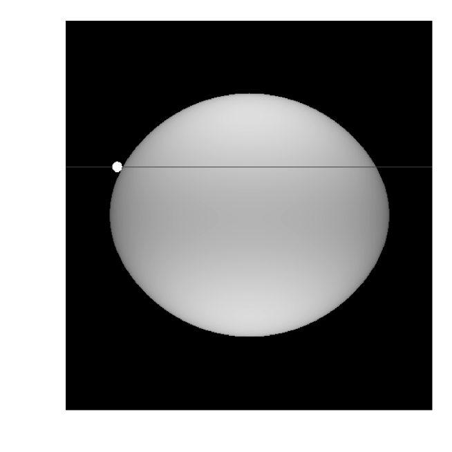
Figure 10: A model representation of the monochromatic intensity in the Kepler band-pass of the rotationally distorted B-star and the small, hot companion star (shown at first contact). The horizontal gray line shows the derived transit path.

We can model the predicted appearance of the B-star based upon our estimates of stellar mass, equatorial radius, rotational period, and average effective temperature. We created a model image of the specific intensity at a wavelength of 6430 Å, which is the centroid of the Kepler instrument response function, using the same methods applied in a study of the rapidly rotating B-star Regulus (McAlister et al. 2005). The star is assumed to have a shape that follows the Roche potential for rotation about a point mass, and each surface element has a specific intensity defined by limb and gravity darkening. The specific intensity of a surface element is set by interpolation in a set of Kurucz model values defined by the local temperature, gravity, and orientation of the surface normal to the line of sight. We found values of the polar radius and temperature that led to our derived equatorial radius and surface average temperature. An image of the rotationally distorted star appears in Figure 10. The resulting model has a ratio of equatorial to critical velocity (where the gravitational and centrifugal accelerations are equal) of 0.74, and the radius varies from $2.30R_{\odot}$ at the poles to $2.81R_{\odot}$ at the equator. The temperature in this model varies between 13.8 kK and 10.8 kK from pole to equator, and gravity likewise varies from $\log g=4.18$ to 3.75. The flux weighted, disk integrated value of gravity is $\log g=3.9$, and this appears to be approximately consistent with the appearance of the H$\gamma$ profile (Fig. 7).

We used this model image to calculate transit light curves. We assumed that the apparent transit path follows a trajectory parallel to the stellar equator with a relative velocity given by $2\pi a/P$. During phases when the disk of the companion is seen projected against the background B-star, we took the flux removed as the product of the companion area and the specific intensity at the projected position of the center of companion (Mandel & Agol 2002; Barnes 2009). For the phases between first and second contact, we assumed that the companion occults a locally linear stellar limb of the B-star with a slope given by the Roche model shown in Figure 10, and the specific intensity was estimated at test positions perpendicular to the local limb to make a numerical calculation of the occulted flux. This constrained model has only two free parameters: the ratio of secondary to primary polar radius $R_{2}/R_{1~{}{\rm polar}}$ and the ratio $z_{0}/R_{1~{}{\rm polar}}$ of the smallest distance $z_{0}$ from the transit trajectory to the center of the B-star relative to the primary polar radius. The value of $R_{2}/R_{1~{}{\rm polar}}$ sets the amount of light removed and hence the depth of the transit light curve, while the value of $z_{0}/R_{1~{}{\rm polar}}$ sets the duration of the transit (longer for transits near the equator with smaller $z_{0}$).

We show in Figure 11 the occultation and transit light curves of KOI-81 from nine months of Kepler short cadence observations. These plots show the photometric fluxes normalized to unity outside of eclipses that we calculated by rebinning and averaging all the available measurements in orbital phase bins equivalent to 3 minutes duration. The Kepler photometry was detrended and pre-whitened for the primary oscillation frequency $f_{1}$ (§5) before rebinning. The upper plot of the total occultation of the hot companion by the B-star indicates that the companion contributes a flux fraction of $F_{2}/F_{1}=0.00501\pm 0.00006$ in the Kepler band-pass, and we renormalized the model for this extra flux in calculating the model transit curves. The model curves were also convolved with a temporal box function to represent the bin size applied to the observations. Our best fit (shown in Fig. 10 and Fig. 11) was obtained with $R_{2}/R_{1~{}{\rm polar}}=0.0426\pm 0.0003$ and $z_{0}/R_{1~{}{\rm polar}}=0.396\pm 0.011$ (equivalent to an orbital inclination of $i=88\fdg 97\pm 0\fdg 04$). The individual transits display asymmetries that appear to be related to the pulsational phases at the times of transit, and because the mean transit curve shown in Figure 11 represents data from only 12 transits, we do not attribute any significance to the trends in the residuals from the fitted transit light curve. We caution that the quoted uncertainties in the fitting parameters do not account for the range in the possible values for the rotation rate we adopted. Nevertheless, it is interesting to note that the derived radius of the companion $R_{2}/R_{\odot}=0.0979\pm 0.0019$ is close to what we list in Table 3 based upon the spherical approximation, mean density, and radius ratio from the Kepler project, and the primary radius given in Table 3 falls comfortably between the polar and equatorial radii of the rotating model.

In §4 we compared the observed and model spectral line depths of the secondary to estimate that the total flux ratio at 1370 Å is $F_{2}/F_{1}=0.05\pm 0.02$, and using the temperatures we derived, we predict that this flux ratio will vary from $F_{2}/F_{1}=0.14$ at 1150 Å to $F_{2}/F_{1}=0.0076$ in the Kepler optical band. The observed flux ratio is approximately related to radius ratio by

$${F_{2}\over F_{1}}={f_{2}\over f_{1}}\left({R_{2}\over R_{1}}\right)^{2}$$ (1)

where $f_{2}/f_{1}$ is the ratio of monochromatic flux per unit area. According to the Kurucz flux models for our stellar parameters, $f_{2}/f_{1}=14.5\pm 0.5$ at 1370 Å, so the observed flux ratio would then imply a radius ratio of $R_{2}/R_{1}=0.059\pm 0.012$. Both the flux and radius ratio estimates from spectroscopy are somewhat larger than the corresponding estimates from the Kepler transit analysis, but the differences are not surprising given the large uncertainties associated with the flux ratio from spectroscopy.

We can also use equation 1 to infer the temperature ratio from the observed flux ratio in the Kepler band. The Kurucz flux models vary as $f\propto T_{\rm eff}^{a}$ with $a=1.58$ for $\log g=5$, $\lambda=6430$ Å, and $T_{\rm eff}$ in the range 10 to 25 kK. Thus, if we set the radius of the primary as $(R_{1~{}{\rm equator}}+R_{1~{}{\rm polar}})/2=1.11R_{1~{}{\rm polar}}$, then we can use the values of $F_{2}/F_{1}$ and $R_{2}/R_{1~{}{\rm polar}}$ from above to find a temperature ratio of $T_{2~{}{\rm eff}}/T_{1~{}{\rm eff}}=2.2$. This is broadly consistent with the temperature estimates from spectroscopy (§4), $T_{2~{}{\rm eff}}/T_{1~{}{\rm eff}}=1.7-2.3$.

7 Discussion

The HST/COS observations of KOI-81 have revealed the spectrum of the hot companion, the stripped down remains of the originally more massive star in the binary. Our derived mass, radius, and temperature values for KOI-81 are consistent with previous results. The mass estimate of the hot, compact companion is slightly lower than earlier estimates ($\sim 0.3M_{\odot}$; van Kerkwijk et al. 2010), solidifying its place among low mass He WDs and their immediate progenitors (with masses below $0.3M_{\odot}$ where WDs have helium cores that are too small to sustain He burning; Silvotti et al. 2012). The radius derived for the subdwarf remains essentially unchanged from earlier estimates, and our analysis confirms that it is larger than typical for He WDs (see Fig. 15 of Panei et al. 2007) like the other thermally bloated WDs found by Kepler (Rappaport et al. 2015). The effective temperature range for the hot companion determined through spectral reconstruction is higher than the previous estimate of Rowe et al. (2010), placing it in the hot subdwarf (sdB) and WD regime. Of the known main sequence (MS) + sdB/He WD binaries, KOI-81 has the hottest, low mass WD (the others range between 9 – 15 kK), although several of the sdB/He WD stars in double degenerate systems have similar effective temperatures (Brown et al. 2013; Hermes et al. 2014).

The relatively long orbital period of KOI-81 suggests that the system widened as the result of conservative mass transfer following the mass ratio reversal. The binary probably began as a relatively close binary, so that mass transfer was initiated as the donor grew in size after concluding core H burning (designated channel 1 in the evolutionary schemes presented by Willems & Kolb 2004). Population synthesis models by Willems & Kolb (2004) show that the post-RLOF systems may frequently have a remnant mass and orbital period like those we find for KOI-81 (see their Fig. 2). The progenitor binaries of such systems typically have similar and low component masses and initial orbital periods somewhat larger than 1 d (see Fig. 2 in Willems & Kolb 2004). For example, van Kerkwijk et al. (2010) present an evolutionary scenario for KOI-81 that begins with a 1.8 and $1.3M_{\odot}$ pair with an orbital period of 1.3 d. It is curious that the dominant pulsation period is similar to this. It may simply be a coincidence, but an alternative possibility is that this pulsation period represents the rotational period of the mass gainer in synchronous rotation before the onset of RLOF. Mass transfer from the donor would subsequently spin up the gainer, but it might take a long time for the angular momentum to be effectively redistributed into the core of the gainer star. We speculate that a slower rotating core may be the source of pulsational wave generation in the envelope of the gainer B-star.

The mass donor remnant may have retained enough of it H-envelope to maintain shell H-burning longer, so that it evolves to hotter temperature before cooling begins (Maxted et al. 2014; Rappaport et al. 2015). Based on the evolutionary scenarios presented by Silvotti et al. (2012) and Rappaport et al. (2015), our derived mass of $0.194\pm 0.020M_{\odot}$ for the hot companion of KOI-81 is consistent with a low mass, pre-He WD that has not yet reached the cooling branch or a He core WD that is already on the cooling branch after experiencing episodes of shell H-burning in CNO flashes. However, when plotted in the ($\log T_{\rm eff},\log g$) plane with the evolutionary sequences for low mass white dwarfs of Althaus et al. (2013), KOI-81 appears to be in an early cooling phase of He core WD evolution. A specific age estimate is difficult to pin down because the star is located in a mass regime which experiences multiple CNO flashes that cause multiple loops in the ($\log T_{\rm eff},\log g$) diagram. Althaus et al. present a grid of masses and cooling ages weighted by the amount of time spent in specific regions of the cooling tracks and the range of masses found in each region. Using the values of $\log T_{\rm eff}$ and $\log g$ derived by van Kerkwijk et al. (2010), they find a mass of $0.196\pm 0.007M_{\odot}$ and cooling age of $372\pm 186$ Myr for KOI-81 (see their Table 2). Our higher values of $\log T_{\rm eff}\approx 4.3$ and $\log g=5.8$ correspond to a mean evolutionary track mass of $0.202\pm 0.015M_{\odot}$ and a cooling age $356\pm 187$ Myr, so our derived stellar parameters are broadly consistent with the evolutionary model predictions.

The evolutionary path of KOI-81 is one of many that create binary systems with low mass WDs. The MS + sdB binaries discovered by Kepler (Rappaport et al. 2015) and WASP (Maxted et al. 2014) represent those systems with stripped-down remnants formed during the first RLOF phase. These occur during the faster part of the pre-He WD evolutionary tracks, but it is easier to detect the low mass WDs at this stage because of their relatively large luminosity (Istrate et al. 2014). In fact, most of the known low mass He WDs are those fainter WDs on the long-lived part of the cooling tracks that are members of binaries with even fainter companions. These are often the remanants of a second mass exchange that involves a common envelope stage. They are generally short period systems that are sdB + WD binaries (Heber et al. 2003; Silvotti et al. 2012), but also include sdB + sdB systems (Ahmad, Jeffery & Fullerton 2004; Kupfer et al. 2015), sdB + neutron star companion (Geier et al. 2009; Istrate et al. 2014), and sdB + substellar companion (Geier et al. 2009; Geier 2015).

The detection of the hot companion in KOI-81 provides us with the means to determine the stellar parameters in one example of what must be a large population of undetected binaries with faint, hot companions (Willems & Kolb 2004; Di Stefano 2011). The fact that the B-star component is also a pulsator opens up the possibility to study the stellar interior of a star that has been radically changed through mass transfer. Furthermore, an analysis of the transit shapes at different phases in the pulsational and rotational cycles may help elucidate the nature of the pulsation modes and source of the rotational modulation (Bíró & Nuspl 2011). The serendipitous discovery of KOI-81 by Kepler has given us the opportunity to explore the properties of stars that have survived transformative mass exchange.

Figure 1: Difference spectra of KOI-81 formed by subtracting the occultation phase spectrum of the primary alone. The sharp absorption lines from the subdwarf star appear near maximum redshift (blueshift) at orbital phase $\phi=0.25$ ($\phi=0.76$). The vertical line segments indicate the positions where interstellar lines were removed from the spectrum.

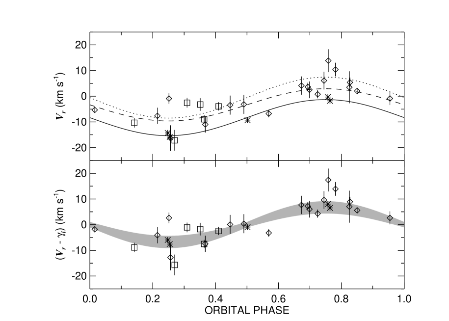
Figure 2: Top panel: The radial velocity data from Table 1 for the primary star plotted as a function of orbital phase. Phase 0.0 corresponds to the time of central transit of the hot subdwarf across the face of the brighter B-type star. The asterisk, diamond, and square symbols represent measurements from COS, TRES, and KPNO, respectively, and the solid, dashed, and dotted lines show preliminary circular fits for the same three sets (with $K_{1}=7.0$, 6.3, and 8.0 km s^-1 and $\gamma_{i}=-8.3$, $-3.4$, and $-0.5$ km s^-1, respectively). Lower panel: The radial velocity differences (formed by subtracting the systemic velocities for each set reported in Table 2) as a function of phase. The shaded region indicates the $\pm 2\sigma$ range in the velocity curve for the adopted fit of the combined measurements.

Figure 3: Radial velocity curves for KOI-81 and its companion. The solid circles and open circles represent the radial velocities derived from COS spectra for the B-star and hot subdwarf, respectively. Plus signs represent the measurements of the B-star velocity from ground-based spectroscopy (see Fig. 2).

Figure 4: The reconstructed UV spectrum of the B-star (solid line) depicted in three successive wavelength panels. The dashed line shows the COS spectrum obtained when the subdwarf was occulted, and it is identical within uncertainties with the reconstructed spectrum. A model spectrum constructed from the UVBLUE grid appears as a dotted line above the reconstructed spectrum (offset by $+0.2$ in units of normalized flux). Several strong absorption lines are identified and marked by the upper vertical line segments, while the lower line segments indicate the locations where interstellar lines were removed from the spectrum.

Figure 5: The reconstructed UV spectrum of the subdwarf star depicted in three successive wavelength panels (in the same format as Fig. 4). The top two panels also show for comparison the spectrum of the hot subdwarf CPD$-64^{\circ}481$ (solid line offset by $+1.3$ in normalized flux).

Figure 6: The spectral energy distribution of the KOI-81 binary including (from short to long wavelength) fluxes from COS (UV), GALEX (NUV), the KPNO 4 m (optical, low resolution spectroscopy), 2MASS (near-IR), and WISE (mid-IR). The solid line depicts a Kurucz atmosphere flux model for the combined system that is based upon a fit of the reddening and the B-star angular diameter.

Figure 7: Left: The Ca II $\lambda 3933$ feature (structured solid line) from the average of the TRES high resolution spectra. A sharp, interstellar component (with a radial velocity of $V_{r}=-19.2\pm 0.9$ km s^-1) is situated near the center of the broad photospheric component. The solid and dotted lines show UVBLUE model profiles for $T_{\rm eff}=10.6$ and 11.7 kK, respectively. Right: The H$\gamma$ line profile (solid line) from an average of the KPNO 4 m moderate resolution spectra. The other lines represent UVBLUE model spectra for three choices of surface gravity.

Figure 9: Top: The broad differential rotation feature at a frequency of about $1.96\sim 2.06$ d^-1 and the adjacent sharp peak $f_{5}=2.08287$ d^-1. Bottom: the same diagram but with the sharp $f_{5}$ peak prewhitened.

Figure 11: The phase-folded light curve of KOI-81 for the occultation of the companion (plus signs, shifted by half an orbit and offset by +0.006 for clarity) and the transit of the companion (dots). The model transit light curve is shown by the solid line.

Table 1: Radial Velocity Measurements

Primary /	Date	Orbital	$V_{r}$	$V_{r}-\gamma_{i}$	$\sigma$	$(O-C)$	Observation
Secondary	(HJD–2,400,000)	Phase	(km s-1)	(km s-1)	(km s-1)	(km s-1)	Source
(1)	(2)	(3)	(4)	(5)	(6)	(7)	(8)
P	55136.6338	0.7248	00+$0.77$	0+$4.31$	1.57	0$-2.34$	TRES
P	55139.6337	0.8504	00+$2.03$	0+$5.57$	0.85	0+$0.13$	TRES
P	55143.5776	0.0156	00$-5.33$	0$-1.79$	0.84	0$-1.13$	TRES
P	55344.8716	0.4464	00$-3.46$	0+$0.08$	3.70	0+$2.30$	TRES
P	55347.8033	0.5692	00$-6.76$	0$-3.22$	1.43	0$-6.05$	TRES
P	55350.7684	0.6934	00+$3.63$	0+$7.17$	1.62	0+$0.86$	TRES
P	55366.7730	0.3637	00$-8.98$	0$-7.52$	1.60	0$-2.43$	KPNO
P	55366.8595	0.3673	0$-11.00$	0$-7.46$	3.13	0$-2.47$	TRES
P	55367.8714	0.4097	00$-3.93$	0$-2.47$	1.59	0+$1.15$	KPNO
P	55369.7871	0.4899	00$-3.17$	0+$0.38$	3.69	0+$0.80$	TRES
P	55374.7716	0.6987	00+$2.49$	0+$6.03$	3.23	0$-0.36$	TRES
P	55375.8748	0.7449	00+$6.08$	0+$9.62$	3.44	0+$2.88$	TRES
P	55376.7460	0.7814	0+$10.38$	+$13.92$	2.65	0+$7.31$	TRES
P	55377.8023	0.8256	00+$3.48$	0+$7.02$	6.23	0+$1.03$	TRES
P	55380.8825	0.9546	00$-0.89$	0+$2.66$	2.53	0+$0.76$	TRES
P	55401.7202	0.8274	00+$5.38$	0+$8.92$	1.86	0+$2.97$	TRES
P	55458.7261	0.2150	00$-7.64$	0$-4.10$	3.15	0+$2.47$	TRES
P	55459.6061	0.2518	00$-0.91$	0+$2.64$	2.08	0+$9.37$	TRES
P	55469.6640	0.6731	00+$4.14$	0+$7.68$	3.54	0+$1.72$	TRES
P	55483.5960	0.2566	0$-16.32$	$-12.78$	4.97	0$-6.05$	TRES
P	55495.5829	0.7586	0+$13.85$	+$17.39$	4.43	+$10.67$	TRES
P	55734.3079	0.7571	00$-0.33$	0+$8.00$	1.09	0+$1.27$	HST/COS
P	55734.4731	0.7640	00$-1.81$	0+$6.52$	1.09	0$-0.19$	HST/COS
P	55775.9626	0.5017	00$-9.31$	0$-0.98$	1.09	0$-1.05$	HST/COS
P	55841.5269	0.2478	0$-14.29$	0$-5.96$	1.09	0+$0.78$	HST/COS
P	55841.6811	0.2542	0$-15.88$	0$-7.55$	1.09	0$-0.81$	HST/COS
P	56077.7512	0.1415	0$-10.35$	0$-8.88$	1.84	0$-3.65$	KPNO
P	56081.7577	0.3093	00$-2.55$	0$-1.08$	1.87	0+$5.19$	KPNO
P	56082.7568	0.3512	00$-3.22$	0$-1.76$	2.45	0+$3.66$	KPNO
P	56486.7101	0.2699	0$-17.15$	$-15.68$	4.03	0$-9.00$	KPNO
S	55734.3079	0.7571	$-102.81$	$\cdots$	2.08	0$-1.54$	HST/COS
S	55734.4731	0.7640	0$-99.37$	$\cdots$	2.12	0+$1.61$	HST/COS
S	55841.5269	0.2478	+$101.12$	$\cdots$	2.42	0+$0.15$	HST/COS
S	55841.6811	0.2542	+$100.74$	$\cdots$	2.81	0$-0.21$	HST/COS

Table 2: Orbital Elements for KOI-81

Element	Value
$P$ (days)	23.8760923
$T_{t}$ (HJD–2,400,000)	54976.07186
$K_{1}$ (km s-1)	$6.74\pm 0.67$
$K_{2}$ (km s-1)	$101.18\pm 0.73$
$\gamma_{1}$[TRES] (km s-1)	$-3.54\pm 0.62$
$\gamma_{1}$[KPNO] (km s-1)	$-1.47\pm 0.68$
$\gamma_{1}$[COS] (km s-1)	$-8.33\pm 0.17$
$\gamma_{2}$[COS] (km s-1)	$-0.19\pm 0.72$
$M_{2}/M_{1}$	$0.0666\pm 0.0066$
$a\sin i$ ($R_{\odot}$)	$50.91\pm 0.47$
rms1 (km s-1)	2.9
rms2 (km s-1)	1.6

Table 3: Stellar Parameters for KOI-81

Parameter	Primary	Secondary
$M/M_{\odot}$	$2.916\pm 0.057$	$0.194\pm 0.020$
$R/R_{\odot}$	$2.447\pm 0.022$	$0.0911\pm 0.0025$
$\log g$ (cgs)	4.13	5.81
$T_{\rm eff}$ (kK)	$11.7\pm 1.5$	$>19.4\pm 2.5$
$V\sin i$ (km s-1)	$296\pm 5$	$<10$

Table 4: Significant Photometric Frequencies

	Frequency ($d^{-1}$)	Amplitude ($10^{-6}$)	Phase (rad/$2\pi$)	S/N	Comment
$f_{1}$	$0.722974\pm 0.000002$	$257.6\pm 4.1$	$0.822\pm 0.001$	$107.4$
$f_{2}$	$1.32403\pm 0.00001$	$33.4\pm 2.8$	$0.34\pm 0.006$	$20.6$	$f_{4}+f_{6}$
$f_{3}$	$1.08445\pm 0.00002$	$22.1\pm 3.2$	$0.98\pm 0.01$	$20.5$	$f_{1}+f_{6}$
$f_{4}$	$0.96250\pm 0.00001$	$34.6\pm 3.6$	$0.22\pm 0.008$	$16.7$
$f_{5}$	$2.08287\pm 0.00001$	$31.4\pm 2.6$	$0.77\pm 0.006$	$11.4$	$f_{rot}$
$f_{6}$	$0.36148\pm 0.00002$	$47.5\pm 7.7$	$0.28\pm 0.01$	$10.6$	$0.5f_{1}$
$f_{7}$	$2.34753\pm 0.00002$	$15.7\pm 2.3$	$0.36\pm 0.01$	$8.0$
$f_{8}$	$0.70933\pm 0.00009$	$6.3\pm 4.2$	$0.96\pm 0.04$	$6.9$
$f_{9}$	$1.74647\pm 0.00006$	$5.8\pm 2.3$	$0.15\pm 0.03$	$6.8$
$f_{10}$	$2.08357\pm 0.00003$	$12.3\pm 2.6$	$0.37\pm 0.05$	$4.5$	$f_{rot}$
$f_{11}$	$4.16643\pm 0.00008$	$4.4\pm 2.4$	$0.08\pm 0.04$	$4.3$	$2f_{rot}$
$f_{12}$	$0.0837\pm 0.0002$	$10.9\pm 4.0$	$0.25\pm 0.02$	$3.2$	$2f_{orb}$
$f_{13}$	$2.08216\pm 0.00003$	$10.4\pm 2.6$	$0.09\pm 0.04$	$3.1$	$f_{rot}$

References

- Ahmad et al. (2004) Ahmad, A., Jeffery, C. S., & Fullerton, A. W. 2004, A&A, 418, 275
- Althaus et al. (2013) Althaus, L. G., Miller Bertolami, M. M., & Córsico, A. H. 2013, A&A, 557, A19
- Bagnuolo et al. (1994) Bagnuolo, W. G., Jr., Gies, D. R., Hahula, M. E., Wiemker, R., & Wiggs, M. S. 1994, ApJ, 423, 446
- Balona (2013) Balona, L. A. 2013, MNRAS, 431, 2240
- Balona (2014) Balona, L. A. 2014, MNRAS, 441, 3543
- Barnes (2009) Barnes, J. W. 2009, ApJ, 705, 683
- Bertone et al. (2008) Bertone, E., Buzzoni, A., Chavez, M., & Rodriguez-Merino, L. H. 2008, A&A, 485, 823
- Bíró & Nuspl (2011) Bíró, I. B., & Nuspl, J. 2011, MNRAS, 416, 1601
- Breton et al. (2012) Breton, R. P., Rappaport, S. A., van Kerkwijk, M. H., & Carter, J. A. 2012, ApJ, 748, 115
- Brown et al. (2013) Brown, W. R., Kilic, M., Allende Prieto, C., Gianninas, A., & Kenyon, S. J. 2013, ApJ, 769, 66
- Buchhave et al. (2010) Buchhave, L. A., Bakos, G. Á., Hartman, J. D., et al. 2010, ApJ, 720, 1118
- Carter et al. (2011) Carter, J. A., Rappaport, S., & Fabrycky, D. 2011, ApJ, 728, 139
- Clausen et al. (2012) Clausen, D., Wade, R. A., Kopparapu, R. K., & O’Shaughnessy, R. 2012, ApJ, 746, 186
- Danforth et al. (2010) Danforth, C. W., Keeney, B. A., Stocke, J. T., Shull, J. M., & Yao, Y. 2010, ApJ, 720, 976
- Di Stefano (2011) Di Stefano, R. 2011, AJ, 141, 142
- Fitzpatrick (1999) Fitzpatrick, E. L. 1999, PASP, 111, 63
- Geier (2015) Geier, S. 2015, Rev. Mod. Astr., 27, in press (arXiv:1503.01625)
- Geier et al. (2009) Geier, S., Heber, U., Edelmann, H., et al. 2009, J. Phys.: Conf. Ser., 172, 012008
- Gies et al. (1998) Gies, D. R., Bagnuolo, W. G., Jr., Ferrara, E. C., et al. 1998, ApJ, 493, 440
- Gies et al. (2008) Gies, D. R., Dieterich, S., Richardson, N. D., et al. 2008, ApJ, 682, L117
- Gray & Corbally (2009) Gray, R. O., & Corbally, C. J. 2009, Stellar Spectral Classification (Princeton: Princeton Univ. Press)
- Green et al. (2012) Green, J. C., Froning, C. S., Osterman, S., et al. 2012, ApJ, 744, 60
- Heber et al. (2003) Heber, U., Edelmann, H., Lisker, T., & Napiwotzki, R. 2003, A&A, 411, L477
- Hermes et al. (2014) Hermes, J. J., Brown, W. R., Kilic, M., et al. 2014, ApJ, 792, 39
- Istrate et al. (2014) Istrate, A. G., Tauris, T. M., Langer, N., & Antoniadis, J. 2014, A&A, 751, L3
- Kallinger et al. (2008) Kallinger, T., Reegen, P., & Weiss, W. W. 2008, A&A, 481, 571
- Kitchatinov & Rüdiger (2009) Kitchatinov, L. L., & Rüdiger, G. 2009, A&A, 504, 303
- Kupfer et al. (2015) Kupfer, T., Geier, S., Heber, U., et al. 2015, A&A, 576, A44
- Lenz & Breger (2005) Lenz, P., & Breger M. 2005, CoAst, 146, 53
- Mandel & Agol (2002) Mandel, K., & Agol, E. 2002, ApJ, 580, L171
- Massa et al. (2013) Massa, D., York, B., Hernandez, S., et al. 2013, COS Data Handbook, Version 2.0 (Baltimore: STScI)
- Maxted et al. (2011) Maxted, P. F. L., Anderson, D. R., Burleigh, M. R., et al. 2011, MNRAS, 418, 1156
- Maxted et al. (2014) Maxted, P. F. L., Bloemen, S., Heber, U., et al. 2014, MNRAS, 437, 1681
- McAlister et al. (2005) McAlister, H. A., ten Brummelaar, T. A., Gies, D. R., et al. 2005, ApJ, 628, 439
- Morbey & Brosterhus (1974) Morbey, C. L., & Brosterhus, E. B. 1974, PASP, 86, 455
- Osterman et al. (2011) Osterman, S., Green, J., Froning, C., et al. 2011, Ap&SS, 335, 257
- O’Toole & Heber (2006) O’Toole, S. J., & Heber, U. 2006, A&A, 452, 579
- Pamyatnykh (1999) Pamyatnykh, A. A. 1999, Acta Astron., 49, 119
- Panei et al. (2007) Panei, J. A., Althaus, L. G., Chen, X., & Han, Z. 2007, MNRAS, 382, 779
- Peters et al. (2013) Peters, G. J., Pewett, T. D., Gies, D, R., Touhami, Y. N., & Grundstrom, E. D. 2013, ApJ, 765, 2
- Rappaport et al. (2009) Rappaport, S., Podsiadlowski, Ph., & Horev, I. 2009, ApJ, 698, 666
- Rappaport et al. (2015) Rappaport, S., Nelson, L., Levine, A., et al. 2015, ApJ, in press (arXiv:1502.02303)
- Rodríguez-Merino et al. (2005) Rodríguez-Merino, L. H., Chavez, M., Bertone, E., & Buzzoni, A. 2005, ApJ, 626, 411
- Rowe et al. (2010) Rowe, J. F., Borucki, W. J., Koch, D., et al. 2010, ApJ, 713, L150
- Savonije (2013) Savonije, G. J. 2013, A&A, 559, A25
- Shafter et al. (1986) Shafter, A. W., Szkody, P., & Thorstensen, J. R. 1986, ApJ, 308, 765
- Silvotti et al. (2012) Silvotti, R., Østensen, R. H., Bloemen, S., et al. 2012, MNRAS, 424, 1752
- Thaller et al. (1995) Thaller, M. L., Bagnuolo, W. G., Jr., Gies, D. R., & Penny, L. R. 1995, ApJ, 448, 878
- Townsend (2005) Townsend, R. H. D. 2005, MNRAS, 364, 573
- van Kerkwijk et al. (2010) van Kerkwijk, M. H., Rappaport, S. A., Breton, R. P., et al. 2010, ApJ, 715, 51
- Wade & Rucinski (1985) Wade, R. A., & Rucinski, S. M. 1985, A&AS, 60, 471
- Willems & Kolb (2004) Willems, B., & Kolb, U. 2004, A&A, 419, 1057
- Zucker (2003) Zucker, S. 2003, MNRAS, 342, 1291
- Zucker et al. (2007) Zucker, S., Mazeh, T., & Alexander, T. 2007, ApJ, 670, 1326