An Exploratory study of Higgs-boson pair production

Abstract

Higgs-boson pair production is well known being capable to probe the trilinear self-coupling of the Higgs boson, which is one of the important ingredients of the Higgs sector itself. Pair production then depends on the top-quark Yukawa coupling $g_{t}^{S,P}$, Higgs trilinear coupling $\lambda_{3H}$, and a possible dim-5 contact-type $ttHH$ coupling $g_{tt}^{S,P}$, which may appear in some higher representations of the Higgs sector. We take into account the possibility that the top-Yukawa and the $ttHH$ couplings involved can be CP violating. We calculate the cross sections and the interference terms as coefficients of the square or the 4th power of each coupling $(g_{t}^{S,P},\,\lambda_{3H},\,g_{tt}^{S,P})$ at various stages of cuts, such that the desired cross section under various cuts can be obtained by simply inputing the couplings. We employ the $HH\to\gamma\gamma b\bar{b}$ decay mode of the Higgs-boson pair to investigate the possibility of disentangle the triangle diagram from the box digram so as to have a clean probe of the trilinear coupling at the LHC. We found that the angular separation between the $b$ and $\bar{b}$ and that between the two photons is useful. We obtain the sensitivity reach of each pair of couplings at the 14 TeV LHC and the future 100 TeV $pp$ machine. Finally, we also comment on using the $b\bar{b}\tau^{+}\tau^{-}$ decay mode in Appendix.

I Introduction

A boson was discovered at the Large Hadron Collider (LHC) atlas ; cms . After almost all the Run I data were analyzed, the measured properties of the new particle are best described by the standard-model (SM) Higgs boson higgcision ; update2014 , which was proposed in 1960s higgs . The most constrained is the gauge-Higgs coupling $C_{v}\equiv g_{HWW}=0.94\,^{+0.11}_{-0.12}$, which is very close to the SM value latest . On the other hand, the relevant top- and bottom-Yukawa couplings are not determined as precisely as $C_{v}$ by the current data. Nevertheless, they are within $30-40\%$ of the SM values latest .

Until now there is no information at all about the self-couplings of the Higgs boson, which emerges from the inner dynamics of the Higgs sector. For example, the trilinear couplings from the SM, two-Higgs doublet models (2HDM), and MSSM are very different from one another. Thus, investigations of the trilinear coupling will shed lights on the dynamics of the Higgs sector. One of the best probes is Higgs-boson-pair production at the LHC. There have been a large number of works of Higgs-pair production in the SM plehn ; baglio ; hh-sm ; loop , in model-independent fashion hh-mi ; 1301.3492 ; contino ; low , and in special models beyond the SM hh-bey and in SUSY hh-susy . In the SM, Higgs-pair production receives contributions from two entangled sources, the triangle and box diagrams. The triangle diagram involves the Higgs self-trilinear coupling and the top-Yukawa coupling while the box diagram involves only the top-Yukawa coupling. In order to probe the effects of the Higgs trilinear coupling, we have to disentangle the triangle diagram from the box diagram. We anticipate that the triangle diagram, which contains an $s$-channel Higgs propagator, does not increase as much as the box diagram as the center-of-mass energy $\sqrt{\hat{s}}\equiv M_{HH}$ increases. Therefore, the box diagram tends to give more energetic Higgs-boson pairs than the triangle diagram. Thus, the opening angle in the decay products of each Higgs boson can be used to isolate the triangle-diagram contribution. Indeed, we found that the angular separation $\Delta R_{\gamma\gamma}$ and $\Delta R_{bb}$ between the decay products of the Higgs-boson pair are very useful variables to disentangle the two sources.

Here we also entertain the possibility of a dimension-5 operator $ttHH$, which can arise from a number of extended Higgs models, including composite Higgs models or some general 2HDM’s. For example, in a general 2HDM we can have a diagram with a $(\bar{t}_{L}t_{R}\varphi)$ vertex and a $(\varphi HH)$ vertex connected by the heavy $\varphi$. When the heavy $\varphi$ is integrated out, we are left with the contact diagram $\bar{t}_{L}t_{R}HH$. The anomalous $ttHH$ coupling can contribute to Higgs-pair production via a triangle diagram. This triangle diagram is similar to the triangle diagram with the trilinear Higgs self coupling, except that it does not have the $s$-channel Higgs propagator. We shall show that the new contact diagram will give terms that can be combined with the terms of the triangle diagram, as in Eq. (4). We note that the kinematic behavior of the triangle diagram induced by the dim-5 $ttHH$ contact interaction is different from that induced by the trilinear Higgs self coupling, because of the absence of the Higgs propagator in the contact diagram.

In this work, we adopt the effective Lagrangian approach, taking the liberty that the involved Higgs-boson couplings can be varied freely within reasonable ranges. The relevant couplings considered in this work are (i) the top-quark Yukawa coupling, (ii) the trilinear Higgs self-coupling, and (iii) the contact-type $ttHH$ coupling. In the top-quark Yukawa and contact-type $ttHH$ interactions, we take into account the possibility of the simultaneous presence of the scalar and pseudoscalar couplings which can signal CP violation. The rationale behind the CP-odd part is that the current data, other than the EDM constraints, cannot restrict the CP-odd part. The EDM constraints, however, depend on a number of assumptions and may therefore be weaken because of cancellation among various CP-violating sources edm . On the other hand, $ttHH$ is a dimension-5 operator, which may originate from a genuine dim-6 operator, e.g., $(\overline{Q_{L}}\Phi t_{R})(\Phi^{\dagger}\Phi)$ after electroweak symmetry breaking, $\Phi=(0,\,(v+H)/\sqrt{2})^{T}$. This operator is thus suppressed only by two powers of higher scale, such that it can give a significant contribution at the LHC energies.

Our strategy is first to find a useful expression for Higgs-boson pair production cross sections in terms of these couplings, see Eq. (7). The coefficient of each term depends on the collider energy $\sqrt{s}$, Higgs decay channels, experimental cuts, etc. Thus, such an expression enables us to easily obtain the cross section under various experimental conditions for arbitrary values of the couplings. Our aim is to extract the information on the Higgs couplings, especially on the Higgs self coupling by exploiting the expression. It is helpful to consider some experimental cuts which can isolate the contribution from the Higgs self coupling and lead to various cross sections with different dependence on the Higgs couplings. In this work, specifically, we employ the $b\bar{b}\gamma\gamma$ decay mode of the Higgs-boson pair and look into the angular separation between the $b$ and $\bar{b}$ and that between the photons. It is shown that one can map out the possible regions of Higgs couplings assuming certain values of measured cross sections, though it is channel dependent. Thanks to the largest branching ratio of the Higgs boson into $b\bar{b}$, the angular separation between the bottom-quark pair is an useful tool in for most of the proposed channel at the LHC.

In summary, the current work marks a number of improvements over previous published works as listed in the following:

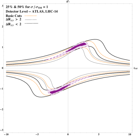
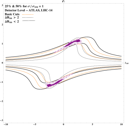
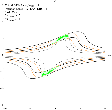
Figure 4: CPC1: The 25% and 50% sensitivity regions bounded by three measurements of cross sections with basic cuts, $\Delta R_{\gamma\gamma}>2$, and $\Delta R_{\gamma\gamma}<2$ (the upper-left panel); with basic cuts, $\Delta R_{bb}>2$, and $\Delta R_{bb}<2$ (the upper-right panel); and basic cuts, $\Delta R_{\gamma\gamma},\,\Delta R_{bb}>2$, and $\Delta R_{\gamma\gamma},\,\Delta R_{bb}<2$ (the lower panel). We assume that the measurements agree with the SM values with uncertainties of 25% and 50%, respectively.

1. We have included the CP-odd part in the top-Yukawa coupling. The CP-even and CP-odd parts are constrained by an elliptical-like equation by the current Higgs-boson data, as shown in Fig. 4 of Ref. update2014 . Note that the effects of the CP-odd part of the top-Yukawa coupling at the LHC, ILC, and photon colliders were studied in Ref. cpodd , though we study the effects in depth for the LHC here.

2. We have included the dim-5 anomalous $ttHH$ contact coupling, as done in Ref. contino ; low . Furthermore, we also include the CP-odd part of this contact coupling.

3. We have calculated an easy-to-use expression to obtain the cross sections as a function of the involved couplings at each center-of-mass energy. We also obtain similar expressions in various kinematic regions such that one can easily obtain the cross sections under the proposed experimental cuts for arbitrary values of the Higgs couplings.

4. With assumed uncertainties in the measurements of cross sections, we can map out the sensitivity regions of parameter space that can be probed at the LHC.

The organization of the work is as follows. In the next section, we describe the formalism for our exploratory approach and present an expression for the Higgs-boson pair production cross section in terms of various combinations of the Higgs couplings under consideration. In Section III, we examine the behavior of each term of the cross section versus energies. In Section IV, employing the $HH\to(\gamma\gamma)(b\bar{b})$ decay mode, we illustrate how to extract the information on the Higgs couplings by exploiting the angular separations between the Higgs decay products. There we also discuss the prospect for the 100 TeV $pp$ machine. We conclude in Section V and offer a few comments with regard to our findings. In Appendix, we compare the SM cross sections at 14 TeV with those at 100 TeV for the process $pp\to H\to\gamma\gamma b\bar{b}$ and give some comments on the $\tau^{+}\tau^{-}b\bar{b}$ decay mode.

II Formalism

Higgs-boson pair production via gluon fusion goes through a triangle diagram with a Higgs-boson propagator and also through a box diagram with colored particles running in it. The relevant couplings involved are top-Yukawa and the Higgs trilinear self coupling. We further explore the possibility of a dim-5 anomalous $ttHH$ contact coupling low . They are given in this Lagrangian:

$$-{\cal L}=\frac{1}{3!}\left(\frac{3M_{H}^{2}}{v}\right)\,\lambda_{3H}\,H^{3}\ +\ \frac{m_{t}}{v}\,\bar{t}\left(g^{S}_{t}+i\gamma_{5}g^{P}_{t}\right)t\,H\ +\ \frac{1}{2}\frac{m_{t}}{v^{2}}\bar{t}\left(g^{S}_{tt}+i\gamma_{5}g^{P}_{tt}\right)t\,H^{2}\,.$$ (1)

In the SM, $\lambda_{3H}=g^{S}_{t}=1$ and $g^{P}_{t}=0$ and $g^{S,P}_{tt}=0$. The differential cross section for the process $g(p_{1})g(p_{2})\to H(p_{3})H(p_{4})$ in the SM was obtained in Ref. plehn as

$$\frac{d\hat{\sigma}(gg\to HH)}{d\hat{t}}=\frac{G_{F}^{2}\alpha_{s}^{2}}{512(2\pi)^{3}}\left[\Big{|}\lambda_{3H}g^{S}_{t}D(\hat{s})F_{\triangle}^{S}+(g^{S}_{t})^{2}F_{\Box}^{SS}\Big{|}^{2}+\Big{|}(g^{S}_{t})^{2}G_{\Box}^{SS}\Big{|}^{2}\right]$$ (2)

where

$$D(\hat{s})=\frac{3M_{H}^{2}}{\hat{s}-M_{H}^{2}+iM_{H}\Gamma_{H}}$$ (3)

and $\hat{s}=(p_{1}+p_{2})^{2}$, $\hat{t}=(p_{1}-p_{3})^{2}$, and $\hat{u}=(p_{2}-p_{3})^{2}$ with $p_{1}+p_{2}=p_{3}+p_{4}$.The loop functions $F_{\triangle}^{S}=F_{\triangle}$, $F_{\Box}^{SS}=F_{\Box}$, and $G_{\Box}^{SS}=G_{\Box}$ with $F_{\triangle\,,\Box}$ and $G_{\Box}$ given in Appendix A.1 of Ref. plehn .

Here we extend the result to including the CP-odd top-Yukawa and the anomalous $ttHH$ couplings:

$$\frac{d\hat{\sigma}(gg\to HH)}{d\hat{t}} = \frac{G_{F}^{2}\alpha_{s}^{2}}{512(2\pi)^{3}}\biggr{\{}\Big{|}\left(\lambda_{3H}g^{S}_{t}D(\hat{s})+g^{S}_{tt}\right)F_{\triangle}^{S}+(g^{S}_{t})^{2}F_{\Box}^{SS}+(g^{P}_{t})^{2}F_{\Box}^{PP}\Big{|}^{2}$$ (4)

$$+ \Big{|}(g^{S}_{t})^{2}G_{\Box}^{SS}+(g^{P}_{t})^{2}G_{\Box}^{PP}\Big{|}^{2}$$

$$+ \Big{|}\left(\lambda_{3H}g^{P}_{t}D(\hat{s})+g^{P}_{tt}\right)F_{\triangle}^{P}+g^{S}_{t}g^{P}_{t}F_{\Box}^{SP}\Big{|}^{2}+\Big{|}g^{S}_{t}g^{P}_{t}G_{\Box}^{SP}\Big{|}^{2}\biggr{\}}\,.$$

More explicitly in terms of each combination of couplings and ignoring the proportionality constant at the beginning of the equation, the above equation becomes

$$\frac{d\hat{\sigma}(gg\to HH)}{d\hat{t}} \propto \lambda_{3H}^{2}|D(\hat{s})|^{2}\left[|F_{\triangle}^{S}|^{2}(g_{t}^{S})^{2}+|F_{\triangle}^{P}|^{2}(g_{t}^{P})^{2}\right]$$ (5)

$$+ 2\lambda_{3H}g_{t}^{S}\Re{\rm e}\left\{D(\hat{s})\left[F_{\triangle}^{S}F_{\Box}^{SS*}(g_{t}^{S})^{2}+(F_{\triangle}^{S}F_{\Box}^{PP*}+F_{\triangle}^{P}F_{\Box}^{SP*})(g_{t}^{P})^{2}\right]\right\}$$

$$+ \left[|F_{\Box}^{SS}|^{2}+|G_{\Box}^{SS}|^{2}\right](g_{t}^{S})^{4}$$

$$+ \left\{2\Re{\rm e}\left[F_{\Box}^{SS}F_{\Box}^{PP*}+G_{\Box}^{SS}G_{\Box}^{PP*}\right]+|F_{\Box}^{SP}|^{2}+|G_{\Box}^{SP}|^{2}\right\}(g_{t}^{S})^{2}(g_{t}^{P})^{2}$$

$$+ \left[|F_{\Box}^{PP}|^{2}+|G_{\Box}^{PP}|^{2}\right](g_{t}^{P})^{4}$$

$$+ |F_{\Delta}^{S}|^{2}(g_{tt}^{S})^{2}+|F_{\Delta}^{P}|^{2}(g_{tt}^{P})^{2}$$

$$+ 2g_{tt}^{S}\left[\lambda_{3H}g^{S}_{t}\Re{\rm e}(D)|F_{\Delta}^{S}|^{2}+(g_{t}^{S})^{2}F_{\Delta}^{S}F_{\Box}^{SS*}+(g_{t}^{P})^{2}F_{\Delta}^{S}F_{\Box}^{PP*}\right]$$

$$+ 2g_{tt}^{P}\left[\lambda_{3H}g^{P}_{t}\Re{\rm e}(D)|F_{\Delta}^{P}|^{2}+g_{s}^{S}g_{t}^{P}F_{\Delta}^{P}F_{\Box}^{SP*}\right]\;,$$

where $F_{\triangle}^{P}=F^{A}_{\triangle}$, $F_{\Box}^{SP}=F_{\Box}$, and $G_{\Box}^{SP}=G_{\Box}$ with $F_{\triangle}^{A}$, $F_{\Box}$ and $G_{\Box}$ given in Appendix A.2 of Ref. plehn while $F_{\Box}^{PP}=F_{\Box}$, and $G_{\Box}^{PP}=G_{\Box}$ with $F_{\Box}$ and $G_{\Box}$ in Appendix A.3 of Ref. plehn . In the heavy quark limit, one may have plehn

$$F_{\triangle}^{S} = +\frac{2}{3}+{\cal O}(\hat{s}/m_{Q}^{2})\,,\ \ \ F_{\Box}^{SS}=-\frac{2}{3}+{\cal O}(\hat{s}/m_{Q}^{2})\,,\ \ \ F_{\Box}^{PP}=+\frac{2}{3}+{\cal O}(\hat{s}/m_{Q}^{2})\,,$$

$$F_{\triangle}^{P} = +1+{\cal O}(\hat{s}/m_{Q}^{2})\,,\ \ \ F_{\Box}^{SP}=-1+{\cal O}(\hat{s}/m_{Q}^{2})\,,$$

$$G_{\Box}^{SS} = G_{\Box}^{PP}=G_{\Box}^{SP}={\cal O}(\hat{s}/m_{Q}^{2})$$ (6)

leading to large cancellation between the triangle and box diagrams.

The production cross section normalized to the corresponding SM cross section, with or without cuts, can be parameterized as follows:

$$\frac{\sigma(gg\to HH)}{\sigma_{\rm SM}(gg\to HH)} = \lambda_{3H}^{2}\left[c_{1}(s)(g^{S}_{t})^{2}+d_{1}(s)(g^{P}_{t})^{2}\right]+\lambda_{3H}g^{S}_{t}\left[c_{2}(s)(g^{S}_{t})^{2}+d_{2}(s)(g^{P}_{t})^{2}\right]$$ (7)

$$+\left[c_{3}(s)(g^{S}_{t})^{4}+d_{3}(s)(g^{S}_{t})^{2}(g^{P}_{t})^{2}+d_{4}(s)(g^{P}_{t})^{4}\right]$$

$$+\lambda_{3H}\left[e_{1}(s)g^{S}_{t}g^{S}_{tt}+f_{1}(s)g^{P}_{t}g^{P}_{tt}\right]+g^{S}_{tt}\left[e_{2}(s)(g^{S}_{t})^{2}+f_{2}(s)(g^{P}_{t})^{2}\right]$$

$$+\left[e_{3}(s)(g^{S}_{tt})^{2}+f_{3}(s)g^{S}_{t}g^{P}_{t}g^{P}_{tt}+f_{4}(s)(g^{P}_{tt})^{2}\right]$$

where the numerical coefficients $c_{1,2,3}(s)$, $d_{1,2,3,4}(s)$, $e_{1,2,3}(s)$, and $f_{1,2,3,4}(s)$ depend on $s$ and experimental selection cuts. Upon our normalization, the ratio should be equal to $1$ when $g_{t}^{S}=\lambda_{3H}=1$ and $g_{t}^{P}=g_{tt}^{S,P}=0$ or $c_{1}(s)+c_{2}(s)+c_{3}(s)=1$. The coefficients $c_{1}(s)$ and $c_{3}(s)$ are for the SM contributions from the triangle and box diagrams, respectively, and the coefficient $c_{2}(s)$ for the interference between them.

Once we have the coefficients $c_{i},d_{i},e_{i}$, and $f_{i}$’s, the cross sections can be easily obtained for any combinations of couplings. Our first task is to obtain the dependence of the coefficients on the collider energy $\sqrt{s}$, Higgs decay channels, experimental cuts, etc.

III Behavior of the cross sections

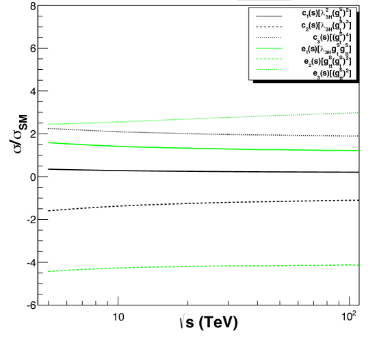
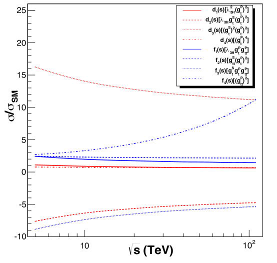
Figure 1: The coeffcients $c_{i}(s)$ and $e_{i}(s)$ (upper) with $i=1,2,3$ and $d_{j}(s)$ and $f_{j}(s)$ (lower) with $j=1,2,3,4$ as functions of $s$.

We first examine the behavior of each piece of cross sections versus energies. We show the coefficients $c_{i},d_{i},e_{i},f_{i}$’s at $\sqrt{s}=8,14,33,100$ TeV in Table 1 and also in Fig. 1 . The triangle diagram involves an $s$-channel Higgs-boson propagator. At center-of-mass energy $\sqrt{\hat{s}}$ considerably higher than $M_{H}$, it behaves like $1/\hat{s}$. Thus the triangle diagram decreases more rapidly than the box and contact diagrams, as reflected from the coefficients $c_{1}$ and $d_{1}$ when $\sqrt{s}$ goes from 8 TeV to 100 TeV. The coefficients $c_{3}$, $d_{3}$ and $d_{4}$ associated with the box diagram more or less remain the same as the energy goes up. On the other hand, the contact diagram involving the coefficients $e_{3}$ and $f_{4}$ increases with energy, in particular tremendous increases in $f_{4}$. It is easy to see that the contact diagram is dim-5 and obviously grows with energy. At certain high enough energy, it may upset unitarity.

We can examine the validity of the anomalous $ttHH$ contact coupling by projecting out the leading partial-wave coefficient for the scattering $t\bar{t}\to HH$. At high energy, the amplitude

$$i{\cal M}(t\bar{t}\to HH)\sim g^{S}_{tt}\frac{m_{t}\sqrt{\hat{s}}}{v^{2}}\;.$$

The leading partial-wave coefficient is given by

$$a_{0}=\frac{1}{64\pi}\int_{-1}^{1}d(\cos\theta)P_{0}(\cos\theta)(i{\cal M})=g^{S}_{tt}\frac{m_{t}\sqrt{\hat{s}}}{32\pi v^{2}}\;.$$

Requiring $|a_{0}|<1/2$ for unitarity we obtain

$$\sqrt{\hat{s}}\leq\frac{17.6}{g_{tt}^{S}}\;{\rm TeV}\;.$$

Therefore, the anomalous $ttHH$ contact term can be safely applied at the LHC for $g_{tt}^{S}\lesssim 3-5$ as most of the collisions occur at $\sqrt{\hat{s}}\lesssim$ a few TeV.

Table 1: The behavior of the coefficients $c_{i}(s)$, $d_{i}(s)$, $e_{i}(s)$, and $f_{i}(s)$ versus collider energy $\sqrt{s}$, see Eq. (7).

$\sqrt{s}$ (TeV)	$c_{1}(s)$	$c_{2}(s)$	$c_{3}(s)$	$d_{1}(s)$	$d_{2}(s)$	$d_{3}(s)$	$d_{4}(s)$
	$\left[\lambda_{3H}^{2}(g_{t}^{S})^{2}\right]$	$\left[\lambda_{3H}(g_{t}^{S})^{3}\right]$	$\left[(g_{t}^{S})^{4}\right]$	$\left[\lambda_{3H}^{2}(g_{t}^{P})^{2}\right]$	$\left[\lambda_{3H}g_{t}^{S}(g_{t}^{P})^{2}\right]$	$\left[(g_{t}^{S})^{2}(g_{t}^{P})^{2}\right]$	$\left[(g_{t}^{P})^{4}\right]$
$8$	$0.300$	$-1.439$	$2.139$	$0.942$	$-6.699$	$14.644$	$0.733$
$14$	$0.263$	$-1.310$	$2.047$	$0.820$	$-5.961$	$13.348$	$0.707$
$33$	$0.232$	$-1.193$	$1.961$	$0.713$	$-5.274$	$12.126$	$0.690$
$100$	$0.208$	$-1.108$	$1.900$	$0.635$	$-4.789$	$11.225$	$0.683$

$\sqrt{s}$ (TeV)	$e_{1}(s)$	$e_{2}(s)$	$e_{3}(s)$	$f_{1}(s)$	$f_{2}(s)$	$f_{3}(s)$	$f_{4}(s)$
	$\left[\lambda_{3H}g_{t}^{S}g_{tt}^{S}\right]$	$\left[g_{tt}^{S}(g_{t}^{S})^{2}\right]$	$\left[(g_{tt}^{S})^{2}\right]$	$\left[\lambda_{3H}g_{t}^{P}g_{tt}^{P}\right]$	$\left[g_{tt}^{S}(g_{t}^{P})^{2}\right]$	$\left[g_{t}^{S}g_{t}^{P}g_{tt}^{P}\right]$	$\left[(g_{tt}^{P})^{2}\right]$
$8$	$1.460$	$-4.313$	$2.519$	$2.104$	$2.350$	$-7.761$	$3.065$
$14$	$1.364$	$-4.224$	$2.617$	$1.848$	$2.269$	$-6.886$	$3.769$
$33$	$1.281$	$-4.165$	$2.783$	$1.622$	$2.207$	$-6.033$	$5.635$
$100$	$1.214$	$-4.137$	$2.974$	$1.474$	$2.154$	$-5.342$	$10.568$

To some extent we have understood the behavior of the triangle, box, and contact diagrams with the center-of-mass energy, which is kinematically equal to the invariant mass $M_{HH}$ of the Higgs-boson pair. One can then uses $M_{HH}$ to enhance or reduce the relative contributions of triangle or box diagrams. The higher the $M_{HH}$ the relatively larger proportion comes from the box and contact diagrams. Since $M_{HH}$ correlates with the boost energy of each Higgs boson, a more energetic Higgs boson will decay into a pair of particles, which have a smaller angular separation between them than a less energetic Higgs boson. Therefore, the angular separation $\Delta R_{ij}$ between the decay products $i,j$ is another useful kinematic variable to separate the contributions among the triangle, box, and contact diagrams.

IV Numerical Analysis

The Lagrangian in Eq. (1) consists of five parameters: the scalar and pseudoscalar parts of the top-Yukawa coupling $g_{t}^{S,P}$, the scalar and pseudoscalar parts of the anomalous contact coupling $g_{tt}^{S,P}$, and the Higgs trilinear coupling $\lambda_{3H}$. In order to facilitate the presentation and understanding of the physics, we study a few scenarios:

1. CPC1–the top-Yukawa coupling involves only the scalar part and the scale in the anomalous contact coupling is very large – only $g_{t}^{S}$ and $\lambda_{3H}$ are relevant. The relevant coefficients are $c_{1}$, $c_{2}$, and $c_{3}$.

2. CPC2–the top-Yukawa and the anomalous contact couplings involve only the scalar part – $g_{t}^{S}$, $g_{tt}^{S}$, and $\lambda_{3H}$ are relevant. The relevant coefficients are $c_{1}$, $c_{2}$, $c_{3}$, $e_{1}$, $e_{2}$, and $e_{3}$.

3. CPV1–the top-Yukawa coupling involves both the scalar and pseudoscalar parts – $g_{t}^{S}$, $g_{t}^{P}$, and $\lambda_{3H}$ are relevant. The relevant coefficients are $c_{1}$, $c_{2}$, $c_{3}$, $d_{1}$, $d_{2}$, $d_{3}$, and $d_{4}$.

4. CPV2–the contact $ttHH$ coupling involves both the scalar and pseudoscalar parts – $g_{tt}^{S}$, $g_{tt}^{P}$, and $\lambda_{3H}$ are relevant while the top-Yukawa coupling is kept at fixed values. In this case, all the coefficients become relevant. In one of the simplest cases with $g^{S}_{t}=1$ and $g^{P}_{t}=0$, for example, the relevant coefficients are $c_{1}$, $c_{2}$, $c_{3}$, $e_{1}$, $e_{2}$, $e_{3}$, and $f_{4}$.

Note that the above scenarios have been studied using different approaches and separately in literature: CPC1 in Ref. 1301.3492 , CPC2 in Ref. contino , and CPV1 in Ref. cpodd . The scenario CPV2 is new with the CP-odd component of the $ttHH$, in which the CP-odd component $g_{tt}^{P}$ of the $ttHH$ coupling appears either with $g_{t}^{P}$ or in square.

We used the CTEQ6L1 cteq with both the renormalization and factorization scales $\mu=M_{H}$ for the parton distribution functions. Since we focus on the ratios relative to the SM predictions, we anticipate the uncertainties due to scale dependence, choice of parton distribution functions, and experimental acceptance are reduced to a minimal level . For the branching ratios of the Higgs boson we employ the values for the SM Higgs boson listed in the LHC Higgs Cross Section Working Group group . Here we ignore the slight variation in the diphoton branching ratio due to the change in the top-Yukawa coupling. This is because we do not want to interfere with the more important goal of the work – interference effects between the triangle and box diagrams and the sensitivity to the trilinear Higgs coupling. For Higgs-pair production we used a modified MADGRAPH implementation loop ; website , which allows us to vary the top-Yukawa, Higgs trilinear, and the contact $ttHH$ couplings.

In this work, we make a working assumption that the $b\bar{b}\gamma\gamma$ background can be estimated with a reasonable accuracy and can be extracted from the experimental data. Once the background is subtracted from the data, we are left with the signal events. In order to do so, we impose a set of basic cuts for the acceptance of the $b$ quarks and photons, and use $B$-tagging according to the ATLAS template in Delphes v.3 delphes3 , as well as an invariant mass window on the $b\bar{b}$ pair and the photon pair around the Higgs boson mass. The basic cuts are

$$p_{T_{\gamma}}>10\,{\rm GeV},\;\;\;p_{T_{b}}>10\,{\rm GeV},\;\;\;|\eta_{\gamma}|<2.5,\;\;\;|\eta_{b}|<2.5,\;\;\;\Delta R_{\gamma\gamma}>0.4,\;\;\;\Delta R_{bb}>0.4,$$

$$|M_{H}-M_{\gamma\gamma}|<15\;{\rm GeV},\;\;\;|M_{H}-M_{bb}|<25\;{\rm GeV},\;\;\;|M_{H}-M_{\tau\tau}|<25\;{\rm GeV}.\;\;\;$$ (8)

Note that in the appendix we shall discuss the feasibility of using the $\tau^{+}\tau^{-}b\bar{b}$ mode. With this set of basic cuts we continue to study the signal events in various kinematical regions separated by $\Delta R_{\gamma\gamma}$ and $\Delta R_{bb}$.

IV.1 CPC1: $g_{t}^{S}$ and $\lambda_{3H}$

This is the simplest scenario to investigate the variation of the triangle and box diagrams with respect to changes in the Yukawa and trilinear couplings. The corresponding coefficients in Eq. (7) are $c_{1},c_{2},c_{3}$. We let the Higgs boson pair decay into

$$HH\to(\gamma\gamma)\;(b\bar{b})\;.$$

Note that if the process is studied without detector simulation, the distributions for other decay channels, like $b\bar{b}\tau\tau$ or $\gamma\gamma\tau\tau$ would be the same. Nevertheless, the resolutions for $b$, $\tau$, and $\gamma$ are quite different in detectors, and so are the backgrounds considered for each decay channel. In the following, we focus on the $\gamma\gamma b\bar{b}$ channel, which has been considered in a number of works.

We use MADGRAPH v.5 madgraph with parton showering by Pythia v.6 pythia , detector simulations using Delphes v.3delphes3 , and the analysis tools by MadAnalysis 5 madana . We have verified that the coefficients $c_{1,2,3}$ using the default, ATLAS, and CMS templates inside Delphes v.3 are within 10% of one another. From now on we employ the ATLAS template in detector simulations. We show the coefficients in Table 2. We will come back to this table a bit later.

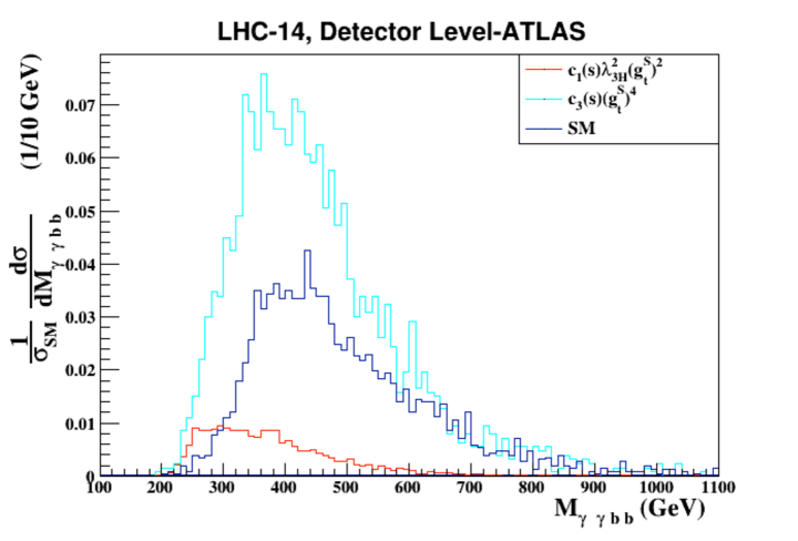
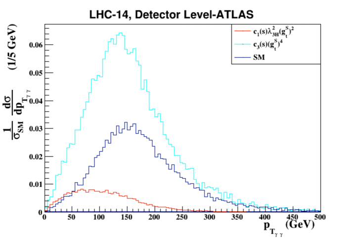
Figure 2: CPC1: Distributions in $M_{\gamma\gamma bb}$ (upper) and $p_{T_{\gamma\gamma}}$ (lower) in the decay products of the Higgs boson pair with detector simulation.

We first look at the distribution of events versus the invariant mass of the Higgs-boson pair via $HH\to\gamma\gamma b\bar{b}$ in Fig. 2 (upper panel) and versus the transverse momentum of the photon pair $p_{T_{\gamma\gamma}}$ (lower panel). In principle, up to detector simulations and higher-order emissions, the transverse momentum distribution of the photon pair is the same as that of the $b\bar{b}$ pair. The triangle diagram (red line) peaks at the lower invariant mass and decreases with $M_{\gamma\gamma b\bar{b}}$, because of the $s$-channel Higgs propagator. The box diagram (skyblue line), on the other hand, is larger than the triangle diagram at high invariant mass. The (darkblue) SM line represents the whole contributions including the destructive interference between the triangle and box diagrams. Similar behavior can be seen in the $p_{T}$ distribution of the photon pair.

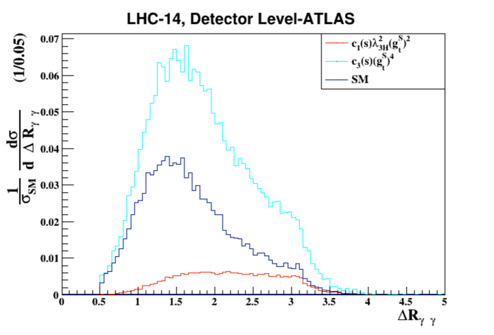
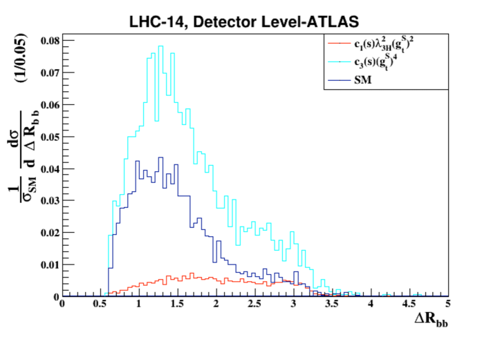
Figure 3: CPC1: Distributions in $\Delta R_{\gamma\gamma}$ (upper) and $\Delta R_{bb}$ (lower) in the decay products of the Higgs boson pair with detector simulation.

Next, we look at the distributions versus $\Delta R_{\gamma\gamma}$ and $\Delta R_{bb}$ in Fig. 3. The lines are the same as in Fig. 2. As we have explained in the previous section, $\Delta R_{\gamma\gamma}$ and $\Delta R_{bb}$ between the decay products of each Higgs boson are useful variables to separate the triangle and box contributions. The angular distribution $\Delta R$ between the two decay products of each Higgs boson correlates with the energy of the Higgs boson, which in turns correlates with the invariant of the Higgs-boson pair. The higher the invariant mass, the more energetic the Higgs boson will be, and the smaller the angular separation between the decay products will be. Therefore, the triangle diagram has wider separation than the box diagram.

It is clear that the distributions of $\Delta R_{\gamma\gamma}$ and $\Delta R_{bb}$ have similar behavior within uncertainties. The box diagram and also the SM, which is dominated by the box contribution, have a peak at $\Delta R_{\gamma\gamma}$ or $\Delta R_{bb}$ less than $2.0$, while the triangle diagram prefers to have the majority at larger $\Delta R_{\gamma\gamma}$ or $\Delta R_{bb}$, say between $2$ and $3$. We therefore come up with (i) $\Delta R_{\gamma\gamma}>2$ ($<2$), (ii) $\Delta R_{bb}>2$ ($<2$), and (iii) $\Delta R_{\gamma\gamma}>2$ and $\Delta R_{bb}>2$ (both $<2$) to enrich the sample of triangle (box) contribution. In the following, we use $\Delta R$ to denote either $\Delta R_{\gamma\gamma}$ or $\Delta R_{bb}$, unless stated distinctively.

We can now look at Table 2, where the coefficients for the ratio of the cross sections $\sigma(gg\to HH)/\sigma_{\rm SM}(gg\to HH)$ as in Eq. (7) are shown. In the CPC1 case, the relevant coefficients are $c_{1}$, $c_{2}$, and $c_{3}$ in which $c_{1}$ is induced by the triangle diagram, $c_{3}$ by the box diagram, and $c_{2}$ by the interference between them. The rows labeled “Basic Cuts” are the ratio of cross sections under the set of cuts in Eq. (8). In the same Table, we also show the coefficients obtained after applying the angular-separation cuts of $\Delta R>2$ or $<2$ and both $\Delta R_{\gamma\gamma,bb}>2$ or $<2$. It is clear that $\Delta R_{\gamma\gamma}>2$ ($<2$) enriches the triangle-diagram (box-diagram) contribution. Similar is true for $\Delta R_{bb}>2$ ($<2$). Further enhancement of triangle diagram can be obtained with both $\Delta R_{\gamma\gamma}>2$ and $\Delta R_{bb}>2$, and vice versa for box diagram.

In the following, we investigate the sensitivity in the parameter space $(g_{t}^{S},\;\lambda_{3H})$ that one can reach at the 14 TeV with 3000 fb^-1 luminosity by using the measurements of cross sections in various kinematical regions. Since we have found that the triangle and box contributions can be distinguished using the $\Delta R$ cuts, we make use of the measured cross sections in the kinematical regions separated by these cuts.

There are two issues that we have to considered when we take the measured cross sections in the kinematical regions. First, the SM backgrounds for the decay channel that we consider, and second, the Next-to-Leading-Order (NLO) corrections hh-nlo . It was shown in Ref. hh-nlo that the NLO and NNLO corrections can be as large as 100% with uncertainty of order 10–20%. The SM backgrounds, on the other hand, can be estimated with uncertainties less than the NNLO corrections. We therefore adopt an approach that the signal cross sections (after background subtraction) are measured with uncertainties of order 25–50%.

About the signal cross sections, the first and the second columns of Table 3 show the SM cross sections for the process $pp\to HH\to\gamma\gamma b\bar{b}$ with detector simulations under various cuts at the 14 TeV LHC . We have taken account of the SM NLO cross section $\sigma_{\rm SM}(pp\to HH)\simeq 34$ fb, the Higgs branching fractions, and both the photon and $b$-quark reconstruction efficiencies with angular-separation cuts of $\Delta R_{bb\,,\gamma\gamma}$. In various kinematical regions depending on the angular cuts, the cross sections range from $\sim 0.001$ fb to $\sim 0.01$ fb. With an integrated luminosity of 3000 fb^-1, we expect of order $30$ signal events when the cross section is 0.01 fb. An estimate of the statistical error is given by the square root of the number of events $\sqrt{N}$, which is then roughly $20\%$ of the total number. Taking into account the uncertainty of order $10-20\%$ from NLO and NNLO corrections, in this work, we use a total uncertainty of $25-50\%$ in the signal cross section in the estimation of sensitivity of the couplings. Our approach is more or less valid except for the case in which both the $\Delta R_{bb}>2$ and $\Delta R_{\gamma\gamma}>2$ cuts are imposed simultaneously. It would be challenging to measure this size of cross section only in the $HH\to\gamma\gamma b\bar{b}$ mode and one may need to combine the measurements in different Higgs-decay channels. Or, one may rely on the future colliders such as a 100 TeV $pp$ machine with larger cross sections and/or higher luminosities.

In Fig. 4, we show the contour lines of $\sigma(gg\to HH)/\sigma_{\rm SM}(gg\to HH)=0.5$ and $1.5$ with the Higgs boson pair decaying into $(\gamma\gamma)(b\bar{b})$. In each panel, we assume three measurements of the ratios corresponding to basic cuts (orange lines), $\Delta R>2$ (dashed black lines), and $\Delta R<2$ (solid black lines): here $\Delta R$ represents $\Delta R_{\gamma\gamma}$ (upper left), $\Delta R_{bb}$ (upper right), or $\Delta R_{\gamma\gamma,bb}$ (lower). Therefore, for example, if the bacis-cuts cross section ratio is measured to be consistent with the SM prediction within $50\%$ error, any points in the two bands bounded by the two pairs of orange lines are allowed. In each band, a rather wide range of $g_{t}^{S}$ and $\lambda_{3H}$ is allowed although they are correlated. Suppose we only make one measurement of the cross section without or with a cut on $\Delta R$, we would not be able to pin down useful values for $g_{t}^{S}$ and $\lambda_{3H}$. However, since the shape of the three bands are not exactly the same, we can make use of three simultaneous measurements in order to obtain more useful information for the couplings $g_{t}^{S}$ and $\lambda_{3H}$.

In the upper-left panel of Fig. 4, we suppose that one can make three measurements of cross sections: with basic cuts, $\Delta R_{\gamma\gamma}>2$, and $\Delta R_{\gamma\gamma}<2$. We assume that the measurements agree with the SM predictions within 25% or 50% uncertainty. The region of parameter space in $(g_{t}^{S},\lambda_{3H})$ bounded by the three measurements is shown by the lighter purple region for 50% uncertainty and darker purple region for 25% uncertainty. Similarly the upper-right panel is for the regions with the $\Delta R_{bb}$ cut. In the lower panel, we show the regions with the combined cuts of $\Delta R_{\gamma\gamma}$ and $\Delta R_{bb}$: both larger than or smaller than 2. The implications from the measurements are very significant. First, all panels show that $g_{t}^{S}$ is significantly away from zero if one can simultaneously measure the cross sections (no matter with 25% or 50% uncertainties) with basic cuts, $\Delta R_{\gamma\gamma}>2$, and $\Delta R_{\gamma\gamma}<2$; and similarly for $\Delta R_{bb}$ and using both distributions. Second, as shown in the lower panel, the value for $\lambda_{3H}$ is statistically distinct from zero if one measures the cross sections with a 25% uncertainty. This is achieved by using both $\Delta R_{\gamma\gamma}$ and $\Delta R_{bb}>2$ or $<2$. Furthermore, from the lower panel in Fig. 4 we can see that with 25% level uncertainty the values of $\lambda_{3H}$ sensitivity regions are $0.3\lesssim|\lambda_{3H}|\lesssim 2.6$.

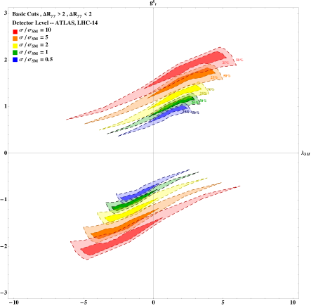
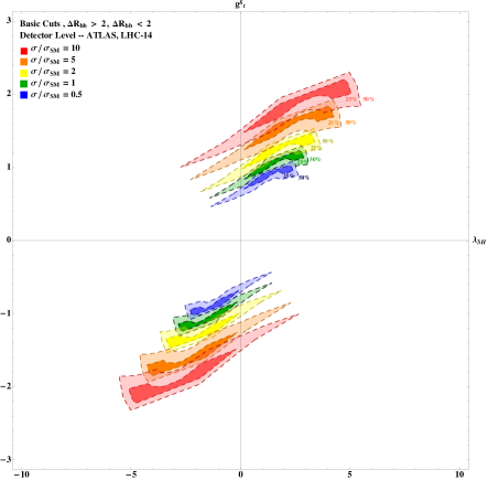
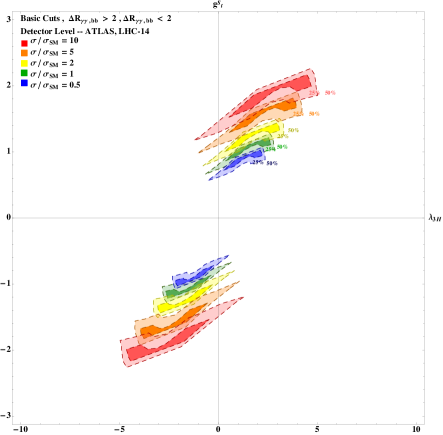
Figure 5: CPC1: The same as Fig. 4 but we assume $\sigma/\sigma_{\rm SM}=0.5-10$.

We can repeat the exercise with the measured cross sections being multiples of the SM predictions. We show the corresponding 25% and 50% regions in Fig. 5 for $\sigma/\sigma_{\rm SM}=0.5,\,1,\,2,\,5,\,10$. Only with both $\Delta R_{\gamma\gamma}$ and $\Delta R_{bb}$, one can really tell if $\lambda_{3H}$ is significantly distinct from zero. The sensitivity regions for $\lambda_{3H}$ for various $\sigma/\sigma_{\rm SM}$ are indicated by the darker color areas.

If the top-Yukawa coupling can be constrained more effectively by Higgs production, by $t\bar{t}H$ production, or by single top with Higgs production in the future measurements, say $g^{S}_{t}=1\pm 0.1$ (10% uncertainty), it can help pinning down the acceptable range of $\lambda_{3H}$. However, even in this case, we emphasize the importance of simultaneous independent measurements, as illustrated in the following argument. In the limit of $g^{S}_{t}=1$, the ratio of the cross sections is given by

$$\frac{\sigma(gg\to HH)}{\sigma_{\rm SM}(gg\to HH)}=c_{1}(s)\,\lambda_{3H}^{2}+c_{2}(s)\,\lambda_{3H}+c_{3}(s)\,.$$ (9)

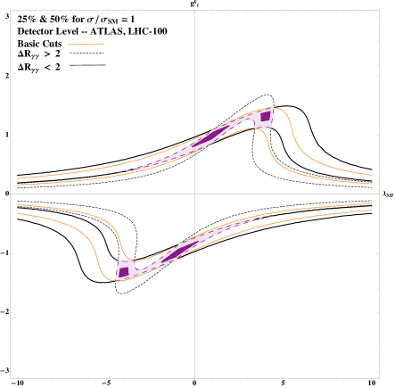
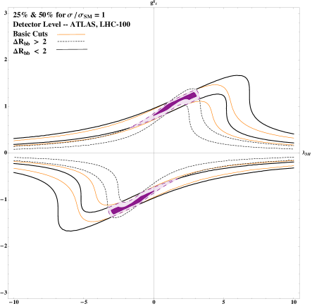
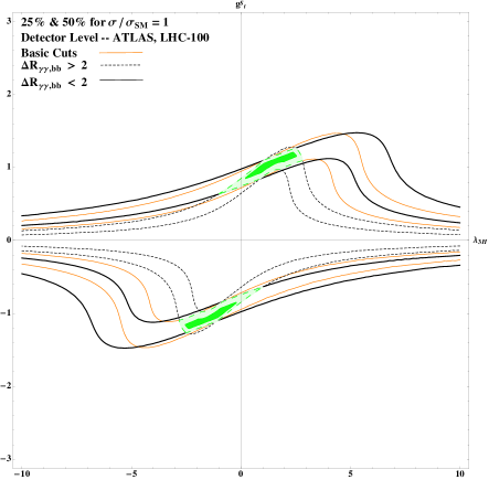
Figure 24: CPC1 at 100 TeV: Exactly the same as Fig. 4, except that it is the case of the 100 TeV $pp$ machine.

Suppose $\sigma(gg\to HH)$ is measured to be the same as $\sigma_{\rm SM}(gg\to HH)$ and then, using the relation $c_{1}(s)+c_{2}(s)+c_{3}(s)=1$, one may find the two solutions for $\lambda_{3H}$: $1$ or $-c_{2}(s)/c_{1}(s)-1$. For example, one may have $\lambda_{3H}=1$ or $4$ at most if only the basic-cuts ratio is measured, see Table 2. Therefore, one cannot determine $\lambda_{3H}$ uniquely with only one measurement even when the measurement is very precise and the exact value of $g^{S}_{t}$ is known. It is unlikely to resolve this two-fold ambiguity at the LHC even we assume the three measurements of the ratios, as shown in Fig. 4. Also, the situation remains the same at the 100 TeV $pp$ machine in which we have $\lambda_{3H}=1$ or $5$ in the bacis-cuts case when $\sigma(gg\to HH)=\sigma_{\rm SM}(gg\to HH)$, see Table 4 and Fig. 24. If a future $e^{+}e^{-}$ linear collider and/or the 100 TeV $pp$ machine are operating in the era of the high-luminosity LHC, combined efforts are desirable to determine the value of $\lambda_{3H}$ uniquely future .

IV.2 CPC2: $g_{t}^{S}$, $\lambda_{3H}$, and $g_{tt}^{S}$

This is the scenario that involves all scalar-type couplings in the triangle, box, and contact diagrams. The corresponding coefficients in Eq. (7) are $c_{1},c_{2},c_{3},e_{1},e_{2},e_{3}$. Results at the detector level using the ATLAS template in Delphes v.3 are shown in Table 2.

We first examine the cross section versus one input parameter at a time, shown in Fig. 6, while keeping the two parameters at their corresponding SM values. In the upper-left panel for $\sigma/\sigma_{\rm SM}$ versus $\lambda_{3H}$, the lowest point occurs at $\lambda_{3H}\approx 2.5$ when the interference term strongly cancels the triangle and box diagrams. Then the ratio increases from the lowest point on either side of $\lambda_{3H}\approx 2.5$. Negative $\lambda_{3H}$s give constructive interference while positive $\lambda_{3H}$s give destructive interference. One may observe similar behavior when $g^{S}_{tt}$ is varied as shown in the lower panel. Taking $\lambda_{3H}=g^{S}_{t}=1$,

$$\frac{\sigma(gg\to HH)}{\sigma_{\rm SM}(gg\to HH)}=e_{3}(s)\,(g^{S}_{tt})^{2}+[e_{2}(s)+e_{1}(s)]\,g^{S}_{tt}+1\,.$$ (10)

Since $e_{1}(s)>0$ and $e_{2}(s)<0$, we see that the contact diagram interferes constructively with the triangle diagram but destructively with the box diagram. The dominance of the box diagram leads to the totally destructive interference when $g^{S}_{tt}>0$, resulting in the minimum at $g^{S}_{tt}\approx 0.5$.

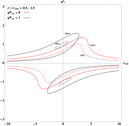
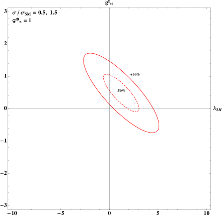
Figure 7: CPC2: Contours marked by $\sigma/\sigma_{\rm SM}=0.5,1.5$ for $(\lambda_{3H},\,g_{t}^{S})$ (upper-left), $(\lambda_{3H},\,g_{tt}^{S})$ (upper-right), and $(g_{t}^{S},\,g_{tt}^{S})$ (lower).

We show contours for the ratio $\sigma/\sigma_{\rm SM}=0.5,1.5$ in the plane of $(\lambda_{3H},\,g_{t}^{S})$ (upper-left), $(\lambda_{3H},\,g_{tt}^{S})$ (upper-right), and $(g_{t}^{S},\,g_{tt}^{S})$ (lower) in Fig. 7. The dashed lines denoted by $-50\%$ is for $\sigma/\sigma_{\rm SM}=0.5$ and those by $+50\%$ for $\sigma/\sigma_{\rm SM}=1.5$. In the upper-left panel in the plane of $(\lambda_{3H},\,g_{t}^{S})$, we show contours for $g_{tt}^{S}=0,1$. The $g_{tt}^{S}=0$ is the same as the SM so that the contours are exactly the same as in Fig. 4, while with $g_{tt}^{S}=1$, the contact diagram contributes significantly to the cross section, so that the contours shift more to negative (positive) $\lambda_{3H}$ for positive (negative) $g_{t}^{S}$. In the upper-right panel, where we show the contours in the plane of $(\lambda_{3H},\,g_{tt}^{S})$, the $g_{tt}^{S}$ negatively correlates with $\lambda_{3H}$ because $e_{1}(s)>0$. In the lower panel, where we fix $\lambda_{3H}=1$, somewhat nontrivial correlation between $g_{t}^{S}$ and $g_{tt}^{S}$ exists.

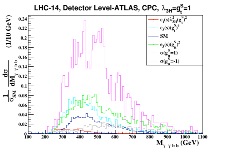
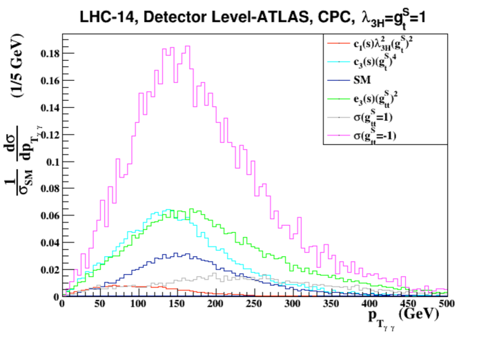
Figure 8: CPC2: Distributions in $M_{\gamma\gamma bb}$ (upper) and $p_{T_{\gamma\gamma}}$ (lower) in the decay products of the Higgs boson pair with detector simulation.

We use the same tools as in the CPC1 case to investigate the decay channel $HH\to\gamma\gamma b\bar{b}$ with parton showering and detector simulations. We first show the invariant mass ($M_{\gamma\gamma b\bar{b}}$) distribution of the Higgs-boson pair and the transverse momentum distribution of the photon pair in Fig. 8. The figure clearly illustrates the behavior of each contributing diagram. The triangle diagram (red lines) peaks at the lower invariant mass and decreases with $M_{\gamma\gamma b\bar{b}}$, because of the $s$-channel Higgs propagator. Then followed by the box diagram (skyblue lines) which is larger than the triangle diagram at high invariant mass. The (darkblue) SM line represents the contributions from the triangle and box diagram including the destructive interference between them. These three distributions are the same as in the CPC1 case. The contact diagram (green lines) shows similar behavior as the box diagram (skyblue lines) at low $M_{\gamma\gamma b\bar{b}}$ and $P_{T_{\gamma\gamma}}$ but with higher and larger tails. The grey and magenta lines represent the full contributions including the destructive and constructive interferences among the triangle, box, and contact diagrams when $g^{S}_{tt}=+1$ and $g^{S}_{tt}=-1$, respectively. The contact diagram is the largest at the high invariant mass. It demonstrates what we describe earlier that the contact diagram grows with energy.

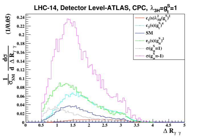
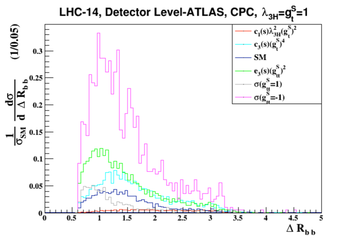
Figure 9: CPC2: Angular distributions of $\Delta R_{\gamma\gamma}$ and $\Delta R_{bb}$ between the two photons and between the two $b$ quarks.

We show the angular distributions $\Delta R_{\gamma\gamma}$ and $\Delta R_{bb}$ between the two decay products of each Higgs boson in Fig. 9. The lines are the same as in Fig. 8. Similar to the CPC1 case, the higher the invariant mass, the more energetic the Higgs boson, and the smaller the angular separation between the decay products will be. Therefore, triangle diagram (red lines) has the widest separation, then followed by the box diagram (skyblue lines), and finally the contact diagram (green lines) has the smallest angular separation. We come up with the similar cuts as in the CPC1 case: $\Delta R$ larger or smaller than $2$ to discriminate the triangle, box, and contact diagrams. We show in Table 2 the coefficients $c_{1},\,c_{2},\,c_{3},\,e_{1},\,e_{2},\,e_{3}$ such that the ratio of cross sections to the SM predictions can be given by Eq. (7).

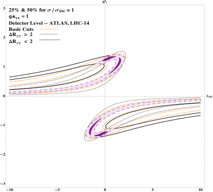
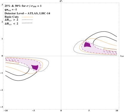
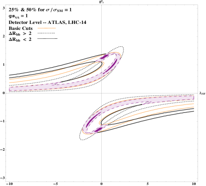
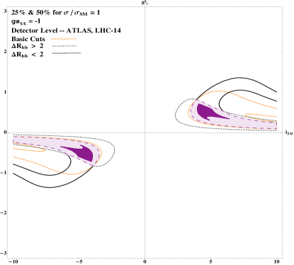
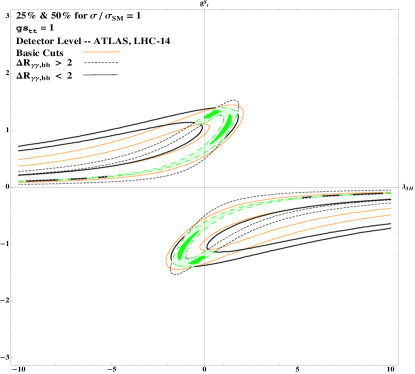
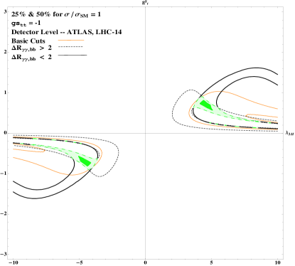
Figure 10: CPC2: The 25% and 50% sensitivity regions in $(\lambda_{3H},g_{t}^{S})$ bounded by three measurements of cross sections with basic cuts, $\Delta R_{\gamma\gamma}>2$, and $\Delta R_{\gamma\gamma}<2$ (the upper panels); with basic cuts, $\Delta R_{bb}>2$, and $\Delta R_{bb}<2$ (the middle panels); and basic cuts, $\Delta R_{\gamma\gamma},\,\Delta R_{bb}>2$, and $\Delta R_{\gamma\gamma},\,\Delta R_{bb}<2$ (the lower panels). The left panels are for $g_{tt}^{S}=1$ while those on the right are for $g_{tt}^{S}=-1$. We assume that the measurements agree with the SM values with uncertainties of 25% and 50%, respectively.

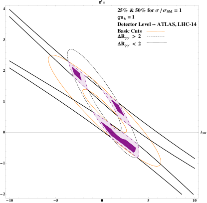
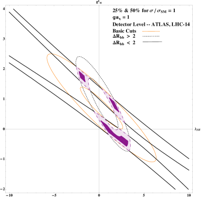
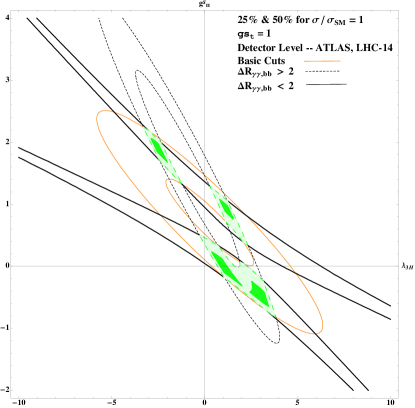
Figure 11: CPC2: similar to Fig. 10 but in the plane of $(\lambda_{3H},\,g_{tt}^{S})$.

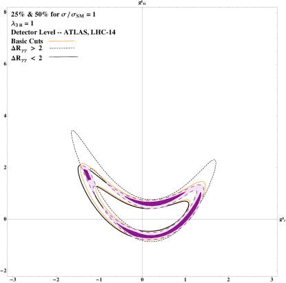
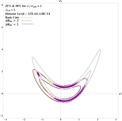
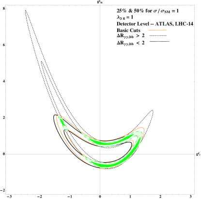
Figure 12: CPC2: similar to Fig. 10 but in the plane of $(g_{t}^{S},\,g_{tt}^{S})$.

Similar to what we have done for CPC1, we can make use of three simultaneous measurements of cross sections with basic cuts, $\Delta R>2$, and $\Delta R<2$. We show the region of parameter space that we can obtain using $\Delta R_{\gamma\gamma}$ (upper panels), $\Delta R_{bb}$ (middle panels), and $\Delta R_{\gamma\gamma}$ and $\Delta R_{bb}$ (lower panels) in the plane of $(\lambda_{3H},\,g_{t}^{S})$ in Fig. 10. Those on the left are for $g_{tt}^{S}=1$ while those on the right are for $g_{tt}^{S}=-1$. Similarly, we show the parameter space in the plane of $(\lambda_{3H},\,g_{t}^{S})$ in Fig. 11 and in the plane of $(g_{t}^{S},\,g_{tt}^{S})$ in Fig. 12.

IV.3 CPV1: $g_{t}^{S}$, $g_{t}^{P}$, and $\lambda_{3H}$

In this scenario, we entertain the possibility that the top Yukawa coupling allows an imaginary part. In most of the measurements of the Higgs boson production cross sections, for example, Higgs boson production cross section via gluon fusion and $t\bar{t}H$ production, both the real and imaginary parts of the coupling come in the form $|g_{t}^{S}|^{2}+|g_{t}^{P}|^{2}$, therefore one cannot tell the phase in the coupling . The relevant coefficients for this CPV1 scenario are $c_{1},c_{2},c_{3},d_{1},d_{2},d_{3},d_{4}$. They are shown in Table 2 at the detector simulation level (ATLAS).

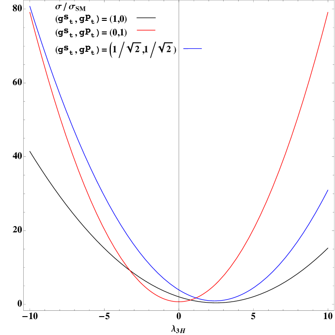
Figure 13: CPV1: The ratio $\sigma/\sigma_{\rm SM}$ versus $\lambda_{3H}$ for $(g_{t}^{S},\,g_{t}^{P})=(1,0),(0,1),(1/\sqrt{2},1/\sqrt{2})$

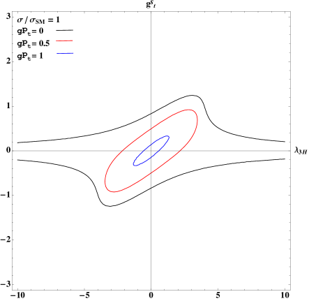
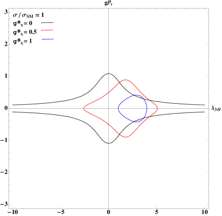
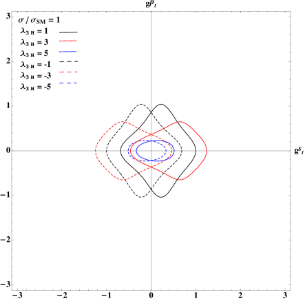
Figure 14: CPV1: Contours for the ratio $\sigma/\sigma_{\rm SM}=1$ in the plane of $(\lambda_{3H},g_{t}^{S})$ (upper-left), $(\lambda_{3H},\,g_{t}^{P})$ (upper-right), and $(g^{S}_{t},g_{t}^{P})$ (lower) for a few values of the third parameter.

We first show the variations of cross sections versus $\lambda_{3H}$ with some fixed values of $g_{t}^{S}$ and $g_{t}^{P}$ in Fig. 13 . Also, the contours for the ratio $\sigma/\sigma_{\rm SM}=1$ in the plane of $(\lambda_{3H},\,g_{t}^{S})$ (upper-left), $(\lambda_{3H},\,g_{t}^{P})$ (upper-right), and $(g_{t}^{S},\,g_{t}^{P})$ (lower) for a few values of the third parameter are shown in Fig. 14.

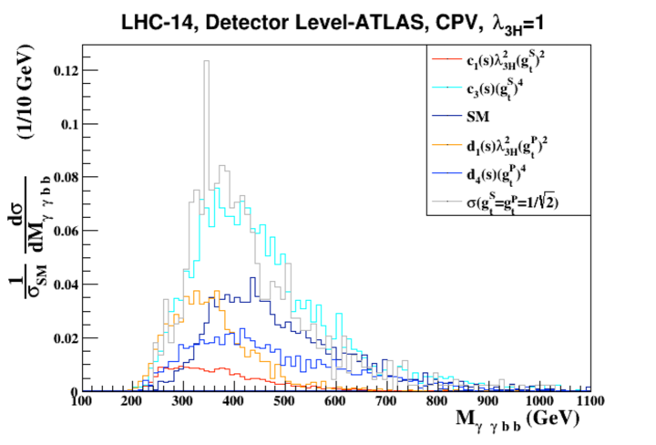
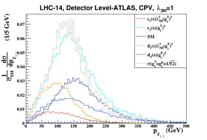
Figure 15: CPV1: Invariant mass distribution $M_{\gamma\gamma bb}$ and $p_{T_{\gamma\gamma}}$ for the decay products of the Higgs-boson pair.

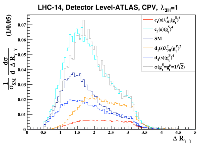
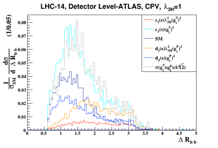
Figure 16: CPV1: Angular distributions of $\Delta R_{\gamma\gamma}$ and $\Delta R_{bb}$ between the two photons and between the two $b$ quarks

Similar to previous two scenarios, we use the same tools to analyze the decay channel $HH\to\gamma\gamma b\bar{b}$ with parton showering and detector simulations. We show the invariant mass $M_{\gamma\gamma b\bar{b}}$ and $p_{T_{\gamma\gamma}}$ in Fig. 15, and the angular distributions $\Delta R_{\gamma\gamma}$ and $\Delta R_{bb}$ between the two decay products of each Higgs boson in Fig. 16.

The terms by the triangle diagram (proportional to $c_{1}$ and $d_{1}$ in red and orange lines, respectively) give the widest separation among all the terms. The terms by the box diagram (proportional to $c_{3}$ and $d_{4}$ in skyblue and blue lines, respectively) give smaller angular separation. The full set of diagrams at the SM values (darkblue lines) and at $g_{t}^{S}=g_{t}^{P}=1/\sqrt{2}$ (grey lines) give similar results as the box diagram.

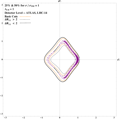
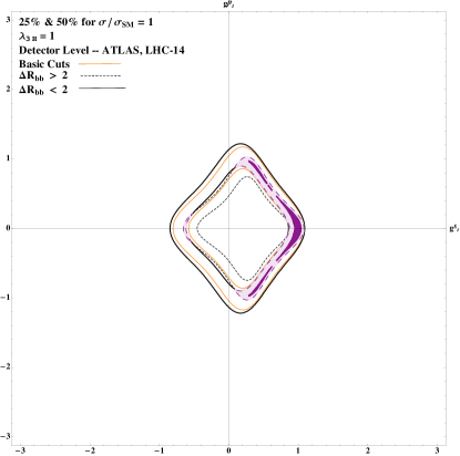
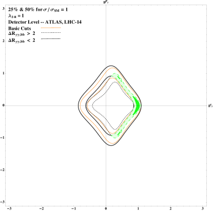
Figure 17: CPV1: The 25% and 50% sensitivity regions in the plane $(g_{t}^{S},\,g_{t}^{P})$ bounded by three measurements of cross sections with basic cuts, $\Delta R_{\gamma\gamma}>2$, and $\Delta R_{\gamma\gamma}<2$ (the upper-left panel); with basic cuts, $\Delta R_{bb}>2$, and $\Delta R_{bb}<2$ (the upper-right panel); and basic cuts, $\Delta R_{\gamma\gamma},\,\Delta R_{bb}>2$, and $\Delta R_{\gamma\gamma},\,\Delta R_{bb}<2$ (the lower panel). We assume that the measurements agree with the SM values with uncertainties of 25% and 50%, respectively.

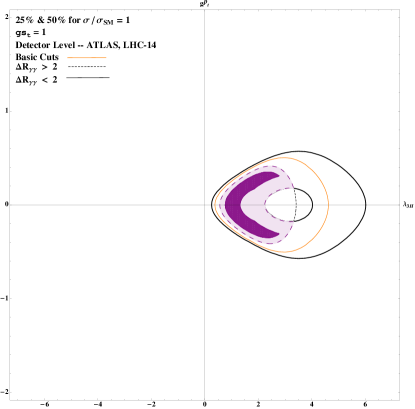
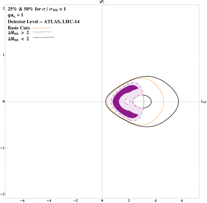
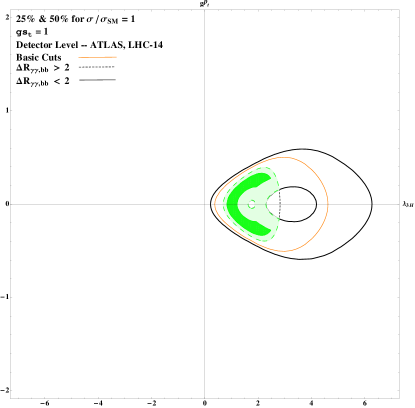
Figure 18: CPV1: similar to Fig. 17 but in the plane of $(\lambda_{3H},\,g_{t}^{P})$.

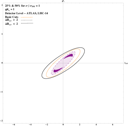
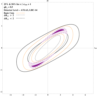
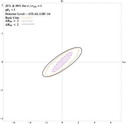
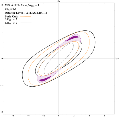
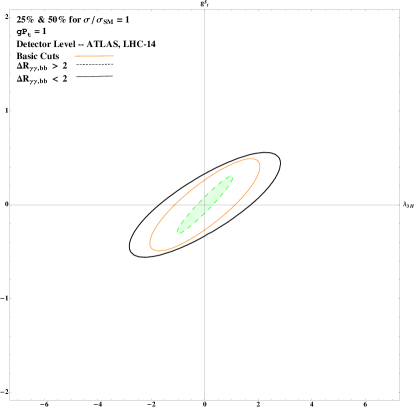
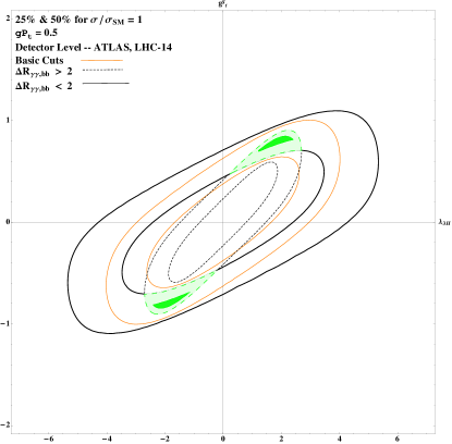
Figure 19: CPV1: similar to Fig. 17 but in the plane of $(\lambda_{3H},\,g_{t}^{S})$. The left panels are for $g_{t}^{P}=1$ while those on the right are for $g_{t}^{P}=0.5$.

Similar to the CPC1 and CPC2 cases, we use the cuts $\Delta R$ larger or smaller than $2$ to discriminate the triangle and box diagrams. We show in Table 2 the coefficients $c_{1},\,c_{2},\,c_{3},\,d_{1},\,d_{2},\,d_{3},d_{4}$, which are relevant ones in the CPV1 scenario, such that the ratio of cross sections to the SM predictions can be obtained by Eq. (7). We show the region of parameter space that we can obtain using $\Delta R_{\gamma\gamma}$, $\Delta R_{bb}$, and $\Delta R_{\gamma\gamma}$ and $\Delta R_{bb}$ in the plane of $(g_{t}^{S},\,g_{t}^{P})$ in Fig. 17, in the plane of $(\lambda_{3H},\,g_{t}^{P})$ in Fig. 18, and in the plane of $(\lambda_{3H},\,g_{t}^{S})$ in Fig. 19.

IV.4 CPV2: $g_{tt}^{S}$, $g_{tt}^{P}$, and $\lambda_{3H}$

Here we study another CP-violating scenario with the CP-even and CP-odd components of the $ttHH$ coupling with the top-Yukawa couplings $g_{t}^{S}$ and $g_{t}^{P}$ at fixed values. Note that the CP-odd coupling $g_{tt}^{P}$ only appears in the product with $g_{t}^{P}$ or by itself squared. In this case, all the coefficients are relevant and they are shown in Table 2 at the detector simulation level (ATLAS).

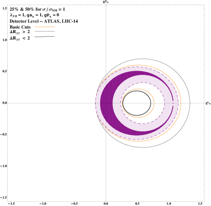
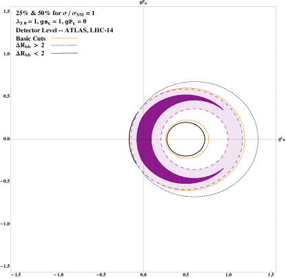
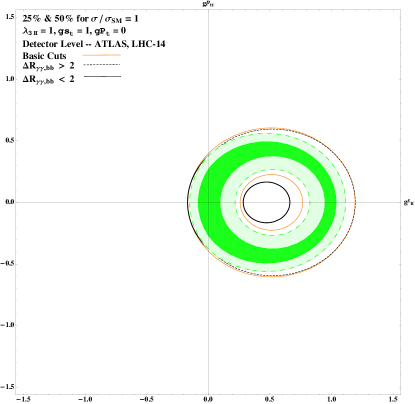
Figure 20: CPV2: The 25% and 50% sensitivity regions in the plane $(g_{tt}^{S},\,g_{tt}^{P})$ (with fixed $\lambda_{3H}=1$, $g_{t}^{S}=1$, and $g_{t}^{P}=0$) bounded by three measurements of cross sections with basic cuts, $\Delta R_{\gamma\gamma}>2$, and $\Delta R_{\gamma\gamma}<2$ (the upper-left panel); with basic cuts, $\Delta R_{bb}>2$, and $\Delta R_{bb}<2$ (the upper-right panel); and basic cuts, $\Delta R_{\gamma\gamma},\,\Delta R_{bb}>2$, and $\Delta R_{\gamma\gamma},\,\Delta R_{bb}<2$ (the lower panel). We assume that the measurements agree with the SM values with uncertainties of 25% and 50%, respectively.

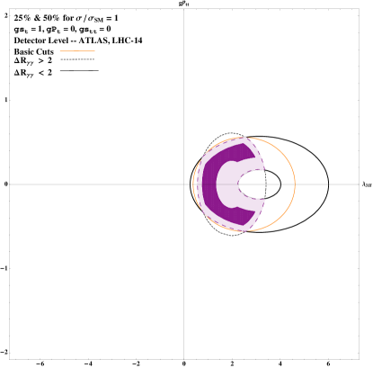
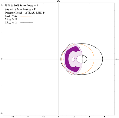
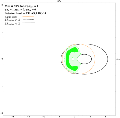
Figure 21: CPV2: similar to Fig. 20 but in the plane of $(\lambda_{3H},\,g_{tt}^{P})$ for $g_{t}^{S}=1$, $g_{t}^{P}=g_{tt}^{S}=0$.

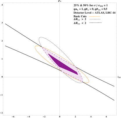
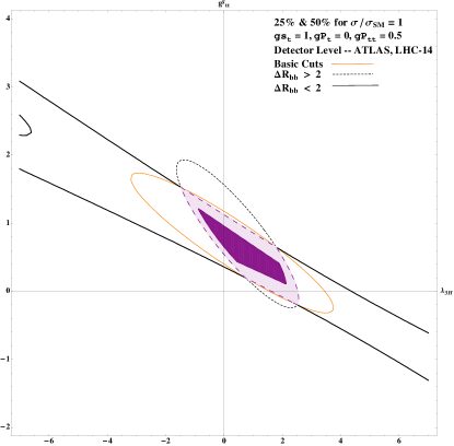
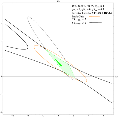
Figure 22: CPV2: similar to Fig. 20 but in the plane of $(\lambda_{3H},\,g_{tt}^{S})$ for $g_{t}^{S}=1$, $g_{t}^{P}=0$, and $g_{tt}^{P}=0.5$.

Similar to previous scenarios we used $HH\to\gamma\gamma b\bar{b}$ with parton showering and detector simulations. We use the cuts $\Delta R$ larger or smaller than 2 to discriminate the triangle and box diagrams. Using the coefficients presented in Table 2, the ratio of cross sections to the SM predictions can be obtained by Eq. (7). We show the region of parameter space that we can obtain using $\Delta R_{\gamma\gamma}$, $\Delta R_{bb}$, and $\Delta R_{\gamma\gamma,bb}$ in the plane of $(g_{tt}^{S},\,g_{tt}^{P})$ for fixed $\lambda_{3H}=1$, $g_{t}^{S}=1$, and $g_{t}^{P}=0$ in Fig. 20; and similarly in the plane of $(\lambda_{3H},\,g_{tt}^{P})$ for $g_{t}^{S}=1$, $g_{t}^{P}=g_{tt}^{S}=0$ in Fig. 21; and finally in the plane of $(\lambda_{3H},\,g_{tt}^{S})$ for $g_{t}^{S}=1$, $g_{t}^{P}=0$, and $g_{tt}^{P}=0.5$ in Fig. 22;

IV.5 100 TeV Prospect

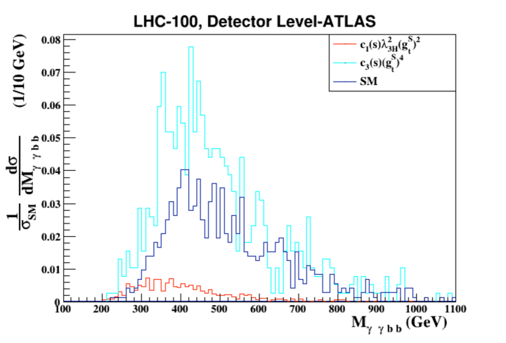
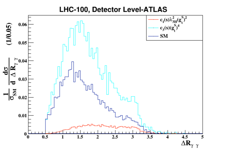
Figure 23: Distributions in the invariant mass distribution $M_{\gamma\gamma bb}$ and the angular separation $\Delta R_{\gamma\gamma}$ in the decay products of the Higgs boson pair with detector simulation at the 100 TeV $pp$ machine.

All the results represented for the 14 TeV run were obtained by manipulating the coefficients represented in Table 2. We represent the coefficients $c_{1,2,3},\,d_{1,2,3,4},\,e_{1,2,3},\,f_{1,2,3,4}$ for the 100 TeV $pp$ machine in Table 4. Just for illustrations, we show the distributions of the invariant mass $M_{\gamma\gamma b\bar{b}}$ and angular separation $\Delta R_{\gamma\gamma}$ for the CPC1 case at the 100 TeV machine in Fig. 23. We found that the behavior of the distributions at 100 TeV is very similar to those at 14 TeV. Therefore, the kinematic regions of interests separated by $\Delta R$ can be taken to be the same as 14 TeV. We can make simultaneous measurements of cross sections at 100 TeV $pp$ machine to isolate the Higgs trilinear coupling. We show the sensitivity regions of parameter space in the CPC1 case at the 100 TeV $pp$ machine in Fig. 24. The regions are very similar to those in 14 TeV, though not exactly the same. Sensitivity reach for each coupling in other cases can be obtained by similar methods with the assumed luminosity.

V Conclusions

In this work, we have studied the behavior of Higgs-boson pair production via gluon fusion at the 14 TeV LHC and the 100 TeV $pp$ machine. We have performed an exploratory study with heavy degrees of freedom being integrated out and resulting in possible modifications of the top-Yukawa coupling, Higgs trilinear coupling, and a new contact $ttHH$ coupling, as well as the potential CP-odd component in the Yukawa and contact couplings. We have identified useful variables – the angular separation between the decay products of the Higgs boson – to discriminate among the contributions from the triangle, box, and contact diagrams. We have successfully demonstrated that with three simultaneous measurements of the Higgs-pair production cross sections, defined by the kinematic cuts, one can statistically show a nonzero value for the Higgs trilinear coupling $\lambda_{3H}$ if we can measure the cross sections with less than 25% uncertainty. This is the key result of this work.

We also offer the following comments with regards to our findings.

1. The triangle diagram, which contains an $s$-channel Higgs propagator, does not increase as much as the box diagram or the contact diagram with the center-of-mass energy $\sqrt{\hat{s}}$. This explains why the opening angle ($\Delta R_{\gamma\gamma}$ or $\Delta R_{bb}$) in the decay products of each Higgs boson is a useful variable to separate between the triangle and the box diagram. Thus, it helps to isolate the Higgs trilinear coupling $\lambda_{3H}$.

2. The contact diagram contains a dim-5 operator $ttHH$, which actually breaks the unitarity at about $\sqrt{\hat{s}}\sim 17.6/g_{tt}^{S}$ TeV. This implies that it could become dominant at high invariant mass.

3. Suppose we take a measurement of cross sections, we can map out the possible region of parameter space. Since in different kinematic regions the regions of parameter space are mapped out differently, such that simultaneous measurements can map out the intersected regions. With measurement uncertainties less than 25% one can statistically show a nonzero value for the Higgs trilinear coupling, and also obtain the sensitivity regions of $\lambda_{3H}$: $0.3\lesssim|\lambda_{3H}|\lesssim 2.6$. for $\sigma/\sigma_{\rm SM}=1$.

4. We found that the behavior of the distributions of the invariant mass $M_{\gamma\gamma b\bar{b}}$ and angular separation $\Delta R_{\gamma\gamma}$ or $\Delta R_{bb}$ at 14 TeV are very similar to those at 100 TeV. We can then use the same method as in 14 TeV to isolate the Higgs trilinear coupling.

5. It is difficult, if not impossible, to determine the Higgs trilinear coupling uniquely at the LHC and 100 TeV $pp$ machine even in the simplest case assuming very high luminosity and precise independent input for the top-Yukawa coupling. We suggest to combine the LHC results with information which can be obtained at a future $e^{+}e^{-}$ linear collider.

6. If the couplings deviate from their SM values, the Higgs-boson pair production cross section can easily increase by an order of magnitude. For example, in the CPC2 case, $\sigma/\sigma_{\rm SM}>10$ for $\lambda_{3H}>9\,{\rm or}\,<-4$ when $g^{S}_{t}=1$ and $g^{S}_{tt}=0$, $g^{S}_{t}>1.7\,{\rm or}\,<-1.3$ when $\lambda_{3H}=1$ and $g^{S}_{tt}=0$, and $g^{S}_{tt}>2.6\,{\rm or}\,<-1.4$ when $\lambda_{3H}=g^{S}_{t}=1$: see Fig. 6. The cross section larger than the SM prediction may reveal the new physics hidden behind the SM and we can have better prospect to measure the Higgs self coupling at the LHC.

Appendix A

In Table 3, we show the SM cross sections for $pp\to HH\to\gamma\gamma b\bar{b}$ at the 14 TeV LHC with and without angular-separation cuts. Note that the cross section before applying any cuts is about $0.09$ fb and it becomes $0.005$ fb after applying the basic cuts. In the region of $\Delta R_{\gamma\gamma}>2(<2)$, the cross section is 0.0013 fb (0.0038 fb) where it is dominated by the triangle (box) diagram. The ratio is about $1:2.8$. We also show the cross sections for the 100 TeV $pp$ machine, and the corresponding ratio is about $1:3.7$. It shows the fact that the triangle diagram is more suppressed because of the $s$-channel Higgs propagator at higher energy. In the regions of $\Delta R_{bb}$ larger and smaller than 2, the ratios are $1:5.7$ and $1:8.2$ at the 14 TeV LHC and the 100 TeV $pp$ machine, respectively.

As we have promised, we are going to comment on the $HH\to\tau^{+}\tau^{-}b\bar{b}$ decay mode. This mode has the obvious advantage of a larger branching ratio than the $\gamma\gamma b\bar{b}$ mode, but the identification efficiency and momentum measurements of $\tau$ leptons are much weaker than photons. In Table 3, we show the SM cross sections for $pp\to HH\to\tau^{+}\tau^{-}b\bar{b}$ at the 14 TeV LHC with and without angular-separation cuts. Taking into account the branching ratios, and the identification and selection efficiencies, the event rates of $\tau^{+}\tau^{-}b\bar{b}$ are similar to those of the $\gamma\gamma b\bar{b}$ mode.

Table 2: 14 TeV LHC: The coeffcients for the ratio of the cross sections $\sigma(gg\to HH)/\sigma_{\rm SM}(gg\to HH)$ as in Eq. (7) with and without the angular-separation cuts of $\Delta R_{\gamma\gamma}>\;{\rm or}<2$; $\Delta R_{bb}>\;{\rm or}<2$; and $\Delta R_{\gamma\gamma}$ and $\Delta R_{bb}$ both $>2$ or $<2$. The relevant coefficients for the CPC1 scenario are $c_{1},\,c_{2},\,c_{3}$; those for the CPC2 scenario are $c_{1},\,c_{2},\,c_{3},e_{1},e_{2},e_{3}$; and those for the CPV1 scenario are $c_{1},\,c_{2},\,c_{3},d_{1},d_{2},d_{3},d_{4}$. All the coefficients are involved in the CPV2 case. Results are at the detector level using the ATLAS template in Delphes v.3.

$\sqrt{s}:14$ TeV	$c_{1}(s)$	$c_{2}(s)$	$c_{3}(s)$	$d_{1}(s)$	$d_{2}(s)$	$d_{3}(s)$	$d_{4}(s)$
Cuts	$\left[\lambda_{3H}^{2}(g_{t}^{S})^{2}\right]$	$\left[\lambda_{3H}(g_{t}^{S})^{3}\right]$	$\left[(g_{t}^{S})^{4}\right]$	$\left[\lambda_{3H}^{2}(g_{t}^{P})^{2}\right]$	$\left[\lambda_{3H}g_{t}^{S}(g_{t}^{P})^{2}\right]$	$\left[(g_{t}^{S})^{2}(g_{t}^{P})^{2}\right]$	$\left[(g_{t}^{P})^{4}\right]$
No cuts	$0.263$	$-1.310$	$2.047$	$0.820$	$-5.961$	$13.348$	$0.707$
Basic Cuts	0.221	-1.104	1.883	0.665	-4.738	11.757	0.650
$\Delta R_{\gamma\gamma}>2$	0.470	-1.868	2.398	1.481	-9.754	19.859	0.858
$\Delta R_{\gamma\gamma}<2$	0.133	-0.834	1.701	0.376	-2.959	8.884	0.576
$\Delta R_{bb}>2$	0.666	-2.512	2.847	2.040	-13.425	25.316	1.074
$\Delta R_{bb}<2$	0.143	-0.857	1.714	0.424	-3.214	9.378	0.575
$\Delta R_{bb}>2\ \&\ \Delta R_{\gamma\gamma}>2$	0.895	-3.150	3.255	2.613	-17.210	30.456	1.278
$\Delta R_{bb}<2\ \&\ \Delta R_{\gamma\gamma}<2$	0.121	-0.785	1.664	0.319	-2.630	8.257	0.563
$\sqrt{s}:14$TeV	$e_{1}(s)$	$e_{2}(s)$	$e_{3}(s)$	$f_{1}(s)$	$f_{2}(s)$	$f_{3}(s)$	$f_{4}(s)$
Cuts	$\left[\lambda_{3H}g_{t}^{S}g_{tt}^{S}\right]$	$\left[g_{tt}^{S}(g_{t}^{S})^{2}\right]$	$\left[(g_{tt}^{S})^{2}\right]$	$\left[\lambda_{3H}g_{t}^{P}g_{tt}^{P}\right]$	$\left[g_{tt}^{S}(g_{t}^{P})^{2}\right]$	$\left[g_{t}^{S}g_{t}^{P}g_{tt}^{P}\right]$	$\left[(g_{tt}^{P})^{2}\right]$
No cuts	$1.364$	$-4.224$	$2.617$	$1.848$	$2.269$	$-6.886$	$3.769$
Basic Cuts	1.381	-3.966	2.521	1.939	2.328	-5.239	3.178
$\Delta R_{\gamma\gamma}>2$	1.857	-4.506	2.267	4.014	2.555	-11.188	2.569
$\Delta R_{\gamma\gamma}<2$	1.212	-3.774	2.611	1.203	2.247	-3.130	3.394
$\Delta R_{bb}>2$	2.248	-5.214	2.474	5.517	3.367	-16.349	3.003
$\Delta R_{bb}<2$	1.229	-3.747	2.529	1.311	2.146	-3.290	3.208
$\Delta R_{bb}>2\ \&\ \Delta R_{\gamma\gamma}>2$	3.047	-5.947	2.780	7.274	3.759	-21.142	3.547
$\Delta R_{bb}<2\ \&\ \Delta R_{\gamma\gamma}<2$	1.238	-3.758	2.664	1.095	2.211	-2.716	3.500

Table 3: The SM cross sections for the process $pp\to HH\to\gamma\gamma b\bar{b}$ with various angular-separation cuts on $\Delta R_{bb\,,\gamma\gamma}$ at the 14 TeV LHC (second column) and at the 100 TeV $pp$ machine (third column). The last column shows them for the process $pp\to HH\to\tau^{+}\tau^{-}b\bar{b}$ at the 14 TeV LHC. We have taken account of the SM NLO cross section $\sigma_{\rm SM}(pp\to HH)\simeq 34$ fb, the Higgs branching fractions, and both the photon and $b$-quark reconstruction efficiencies. The $p_{T}$ dependence of $b$-tagging efficiency is considered and $0.5$ is taken for the $\tau$-tagging efficiency. Also considered is the mis-tagging probability of $P_{j\rightarrow\tau}=0.01$. Results are at the detector level using the ATLAS template in Delphes v.3.

Cuts	SM-14$~{}(\gamma\gamma b\bar{b})~{}~{}~{}~{}$	SM-100$~{}(\gamma\gamma b\bar{b})~{}~{}~{}~{}$	SM-14$~{}(\tau^{+}\tau^{-}b\bar{b})~{}~{}~{}~{}$
	Cross Section (fb)
No cuts	$8.92\times 10^{-2}$	3.73	2.41
Basic Cuts	$5.1\times 10^{-3}$	$2.05\times 10^{-1}$	$3.53\times 10^{-3}$
$\Delta R_{\gamma\gamma/\tau^{+}\tau^{-}}>2$	$1.34\times 10^{-3}$	$4.34\times 10^{-2}$	$6.43\times 10^{-4}$
$\Delta R_{\gamma\gamma/\tau^{+}\tau^{-}}<2$	$3.76\times 10^{-3}$	$1.61\times 10^{-1}$	$2.89\times 10^{-3}$
$\Delta R_{bb}>2$	$7.61\times 10^{-4}$	$2.23\times 10^{-2}$	$4.82\times 10^{-4}$
$\Delta R_{bb}<2$	$4.34\times 10^{-3}$	$1.83\times 10^{-1}$	$3.05\times 10^{-3}$
$\Delta R_{bb}>2\ \&\ \Delta R_{\gamma\gamma/\tau^{+}\tau^{-}}>2~{}~{}~{}~{}$	$4.79\times 10^{-4}$	$1.40\times 10^{-2}$	$3.21\times 10^{-4}$
$\Delta R_{bb}<2\ \&\ \Delta R_{\gamma\gamma/\tau^{+}\tau^{-}}<2~{}~{}~{}~{}$	$3.48\times 10^{-3}$	$1.53\times 10^{-1}$	$2.73\times 10^{-3}$

Table 4: 100 TeV $pp$ machine: The coeffcients for the ratio of the cross sections $\sigma(gg\to HH)/\sigma_{\rm SM}(gg\to HH)$ as in Eq. (7) with and without the angular-separation cuts of $\Delta R_{\gamma\gamma}>\;{\rm or}<2$; $\Delta R_{bb}>\;{\rm or}<2$; and $\Delta R_{\gamma\gamma}$ and $\Delta R_{bb}$ both $>2$ or $<2$. The relevant coefficients for the CPC1 scenario are $c_{1},\,c_{2},\,c_{3}$; those for the CPC2 scenario are $c_{1},\,c_{2},\,c_{3},e_{1},e_{2},e_{3}$; and those for the CPV1 scenario are $c_{1},\,c_{2},\,c_{3},d_{1},d_{2},d_{3},d_{4}$. All the coefficients are involved in the CPV2 case. Results are at the detector level using the ATLAS template in Delphes v.3.

$\sqrt{s}:100$ TeV	$c_{1}(s)$	$c_{2}(s)$	$c_{3}(s)$	$d_{1}(s)$	$d_{2}(s)$	$d_{3}(s)$	$d_{4}(s)$
Cuts	$\left[\lambda_{3H}^{2}(g_{t}^{S})^{2}\right]$	$\left[\lambda_{3H}(g_{t}^{S})^{3}\right]$	$\left[(g_{t}^{S})^{4}\right]$	$\left[\lambda_{3H}^{2}(g_{t}^{P})^{2}\right]$	$\left[\lambda_{3H}g_{t}^{S}(g_{t}^{P})^{2}\right]$	$\left[(g_{t}^{S})^{2}(g_{t}^{P})^{2}\right]$	$\left[(g_{t}^{P})^{4}\right]$
No cuts	$0.208$	$-1.108$	$1.900$	$0.635$	$-4.789$	$11.225$	$0.683$
Basic Cuts	0.173	-1.032	1.860	0.503	-4.045	10.019	0.633
$\Delta R_{\gamma\gamma}>2$	0.389	-1.904	2.515	1.275	-6.972	13.375	0.853
$\Delta R_{\gamma\gamma}<2$	0.115	-0.798	1.683	0.295	-3.258	9.116	0.574
$\Delta R_{bb}>2$	0.607	-2.419	2.813	1.845	-9.336	17.393	1.057
$\Delta R_{bb}<2$	0.120	-0.863	1.743	0.340	-3.400	9.119	0.581
$\Delta R_{bb}>2\ \&\ \Delta R_{\gamma\gamma}>2$	0.753	-2.662	2.909	2.248	-10.518	17.691	1.245
$\Delta R_{bb}<2\ \&\ \Delta R_{\gamma\gamma}<2$	0.102	-0.733	1.632	0.249	-3.041	8.700	0.565
$\sqrt{s}:100$TeV	$e_{1}(s)$	$e_{2}(s)$	$e_{3}(s)$	$f_{1}(s)$	$f_{2}(s)$	$f_{3}(s)$	$f_{4}(s)$
Cuts	$\left[\lambda_{3H}g_{t}^{S}g_{tt}^{S}\right]$	$\left[g_{tt}^{S}(g_{t}^{S})^{2}\right]$	$\left[(g_{tt}^{S})^{2}\right]$	$\left[\lambda_{3H}g_{t}^{P}g_{tt}^{P}\right]$	$\left[g_{tt}^{S}(g_{t}^{P})^{2}\right]$	$\left[g_{t}^{S}g_{t}^{P}g_{tt}^{P}\right]$	$\left[(g_{tt}^{P})^{2}\right]$
No cuts	$1.214$	$-4.137$	$2.974$	$1.474$	$2.154$	$-5.342$	$10.568$
Basic Cuts	1.170	-4.081	2.848	1.300	1.935	-3.379	7.802
$\Delta R_{\gamma\gamma}>2$	1.782	-4.886	2.591	3.675	2.151	-2.696	5.511
$\Delta R_{\gamma\gamma}<2$	1.006	-3.865	2.917	0.662	1.878	-3.563	8.419
$\Delta R_{bb}>2$	2.011	-5.585	2.957	6.947	2.576	-4.961	5.373
$\Delta R_{bb}<2$	1.068	-3.898	2.834	0.612	1.857	-3.186	8.099
$\Delta R_{bb}>2\ \&\ \Delta R_{\gamma\gamma}>2$	2.483	-5.858	3.106	8.165	2.694	-4.722	6.079
$\Delta R_{bb}<2\ \&\ \Delta R_{\gamma\gamma}<2$	0.995	-3.798	2.928	0.437	1.851	-3.466	8.647

Figure 6: CPC2: Variation of the ratio $\sigma/\sigma_{\rm SM}$ using Eq. (7) versus $\lambda_{3H}$ (upper-left), $g_{t}^{S}$ (upper-right), and $g_{tt}^{S}$ (lower) while keeping the other two parameters at their corresponding SM values.

References

- (1) G. Aad et al. [ATLAS Collaboration], Phys. Lett. B 716, 1 (2012) [arXiv:1207.7214 [hep-ex]].
- (2) S. Chatrchyan et al. [CMS Collaboration], Phys. Lett. B 716, 30 (2012) [arXiv:1207.7235 [hep-ex]].
- (3) See for example, K. Cheung, J. S. Lee and P. -Y. Tseng, JHEP 1305, 134 (2013) [arXiv:1302.3794 [hep-ph]].
- (4) K. Cheung, J. S. Lee and P. Y. Tseng, Phys. Rev. D 90, no. 9, 095009 (2014) [arXiv:1407.8236 [hep-ph]].
- (5) P. W. Higgs, Phys. Rev. Lett. 13, 508 (1964); F. Englert and R. Brout, Phys. Rev. Lett. 13, 321 (1964); G. S. Guralnik, C. R. Hagen and T. W. B. Kibble, Phys. Rev. Lett. 13, 585 (1964).
- (6) ATLAS Coll., “Measurements of the Higgs boson production and decay rates and couplings using pp collision data at sqrt(s) = 7 and 8 TeV in the ATLAS experiment”, ATLAS-CONF-2015-007 (March 2015); V. Khachatryan et al. [CMS Collaboration], Eur. Phys. J. C 75, no. 5, 212 (2015) [arXiv:1412.8662 [hep-ex]].
- (7) T. Plehn, M. Spira and P. M. Zerwas, Nucl. Phys. B 479, 46 (1996) [Erratum-ibid. B 531, 655 (1998)] [hep-ph/9603205].
- (8) J. Baglio, A. Djouadi, R. Gröber, M. M. Mühlleitner, J. Quevillon and M. Spira, JHEP 1304, 151 (2013) [arXiv:1212.5581 [hep-ph]].
- (9) C. Englert, F. Krauss, M. Spannowsky and J. Thompson, Phys. Lett. B 743, 93 (2015) [arXiv:1409.8074 [hep-ph]]; T. Liu and H. Zhang, arXiv:1410.1855 [hep-ph]; D. E. Ferreira de Lima, A. Papaefstathiou and M. Spannowsky, JHEP 1408, 030 (2014) [arXiv:1404.7139 [hep-ph]]; V. Barger, L. L. Everett, C. B. Jackson and G. Shaughnessy, Phys. Lett. B 728, 433 (2014) [arXiv:1311.2931 [hep-ph]]; E. Asakawa, D. Harada, S. Kanemura, Y. Okada and K. Tsumura, Phys. Rev. D 82, 115002 (2010) [arXiv:1009.4670 [hep-ph]]; A. Papaefstathiou, L. L. Yang and J. Zurita, Phys. Rev. D 87, no. 1, 011301 (2013) [arXiv:1209.1489 [hep-ph]]; A. Papaefstathiou, arXiv:1504.04621 [hep-ph].
- (10) R. Frederix, S. Frixione, V. Hirschi, F. Maltoni, O. Mattelaer, P. Torrielli, E. Vryonidou and M. Zaro, Phys. Lett. B 732, 142 (2014) [arXiv:1401.7340 [hep-ph]].
- (11) K. Nishiwaki, S. Niyogi and A. Shivaji, JHEP 1404, 011 (2014) [arXiv:1309.6907 [hep-ph]]; M. Gouzevitch, A. Oliveira, J. Rojo, R. Rosenfeld, G. P. Salam and V. Sanz, JHEP 1307, 148 (2013) [arXiv:1303.6636 [hep-ph]]; M. J. Dolan, C. Englert and M. Spannowsky, JHEP 1210, 112 (2012) [arXiv:1206.5001 [hep-ph]]; A. Azatov, R. Contino, G. Panico and M. Son, arXiv:1502.00539 [hep-ph]; N. Liu, S. Hu, B. Yang and J. Han, JHEP 1501, 008 (2015) [arXiv:1408.4191 [hep-ph]]; F. Goertz, A. Papaefstathiou, L. L. Yang and J. Zurita, JHEP 1504, 167 (2015) [arXiv:1410.3471 [hep-ph]]; R. Grober, M. Muhlleitner, M. Spira and J. Streicher, arXiv:1504.06577 [hep-ph];
- (12) F. Goertz, A. Papaefstathiou, L. L. Yang and J. Zurita, JHEP 1306, 016 (2013) [arXiv:1301.3492 [hep-ph]];
- (13) R. Contino, M. Ghezzi, M. Moretti, G. Panico, F. Piccinini and A. Wulzer, JHEP 1208, 154 (2012) [arXiv:1205.5444 [hep-ph]];
- (14) C. R. Chen and I. Low, Phys. Rev. D 90, no. 1, 013018 (2014) [arXiv:1405.7040 [hep-ph]].
- (15) S. Dawson, E. Furlan and I. Lewis, Phys. Rev. D 87, no. 1, 014007 (2013) [arXiv:1210.6663 [hep-ph]]; M. Gillioz, R. Grober, C. Grojean, M. Muhlleitner and E. Salvioni, JHEP 1210 (2012) 004 [arXiv:1206.7120 [hep-ph]]; V. Barger, L. L. Everett, C. B. Jackson, A. Peterson and G. Shaughnessy, Phys. Rev. Lett. 114, 011801 (2015) [arXiv:1408.0003 [hep-ph]]; M. J. Dolan, C. Englert and M. Spannowsky, Phys. Rev. D 87 (2013) 5, 055002 [arXiv:1210.8166 [hep-ph]]; G. D. Kribs and A. Martin, Phys. Rev. D 86, 095023 (2012) [arXiv:1207.4496 [hep-ph]]; A. Arhrib, R. Benbrik, C. H. Chen, R. Guedes and R. Santos, JHEP 0908, 035 (2009) [arXiv:0906.0387 [hep-ph]]; C. O. Dib, R. Rosenfeld and A. Zerwekh, JHEP 0605, 074 (2006) [hep-ph/0509179]; R. Grober and M. Muhlleitner, JHEP 1106, 020 (2011) [arXiv:1012.1562 [hep-ph]]; J. M. No and M. Ramsey-Musolf, Phys. Rev. D 89, no. 9, 095031 (2014) [arXiv:1310.6035 [hep-ph]]; B. Hespel, D. Lopez-Val and E. Vryonidou, JHEP 1409, 124 (2014) [arXiv:1407.0281 [hep-ph]].
- (16) C. Han, X. Ji, L. Wu, P. Wu and J. M. Yang, JHEP 1404, 003 (2014) [arXiv:1307.3790 [hep-ph]]; U. Ellwanger, JHEP 1308, 077 (2013) [arXiv:1306.5541 [hep-ph]]; J. Cao, Z. Heng, L. Shang, P. Wan and J. M. Yang, JHEP 1304, 134 (2013) [arXiv:1301.6437 [hep-ph]]; B. Bhattacherjee and A. Choudhury, Phys. Rev. D 91, no. 7, 073015 (2015) [arXiv:1407.6866 [hep-ph]].
- (17) K. Cheung, J. S. Lee, E. Senaha and P. Y. Tseng, JHEP 1406, 149 (2014) [arXiv:1403.4775 [hep-ph]].
- (18) See N. Liu, S. Hu, B. Yang and J. Han in Ref. hh-mi .
- (19) J. Pumplin, D. R. Stump, J. Huston, H. L. Lai, P. M. Nadolsky and W. K. Tung, JHEP 0207, 012 (2002) [hep-ph/0201195].
-
(20)
LHC Higgs Cross Section Working Group,
https://twiki.cern.ch/twiki/bin/view/LHCPhysics/CrossSections - (21) G. Aad et al. [ATLAS Collaboration], Phys. Rev. D 90, no. 11, 112015 (2014) [arXiv:1408.7084 [hep-ex]].
- (22) V. Khachatryan et al. [CMS Collaboration], Eur. Phys. J. C 74, no. 10, 3076 (2014) [arXiv:1407.0558 [hep-ex]].
-
(23)
For more information please see
https://cp3.irmp.ucl.ac.be/projects/madgraph/wiki/HiggsPairProduction - (24) MADGRAPH: J. Alwall, M. Herquet, F. Maltoni, O. Mattelaer and T. Stelzer, JHEP 1106, 128 (2011) [arXiv:1106.0522 [hep-ph]].
- (25) J. Alwall and the CP3 development team, The MG/ME Pythia-PGS package; the Madgraph at http://madgraph.hep.uiuc.edu/; Pythia at https://pythia6.hepforge.org/; and PGS at http://www.physics.ucdavis.edu/conway/research/software/pgs/pgs4-general.htm.
- (26) J. de Favereau et al. [DELPHES 3 Collaboration], JHEP 1402, 057 (2014) [arXiv:1307.6346 [hep-ex]].
- (27) E. Conte, B. Fuks and G. Serret, Comput. Phys. Commun. 184 (2013) 222 [arXiv:1206.1599 [hep-ph]]; E. Conte, B. Dumont, B. Fuks and C. Wymant, arXiv:1405.3982 [hep-ph].
- (28) S. Dawson, S. Dittmaier and M. Spira, Phys. Rev. D 58, 115012 (1998) [hep-ph/9805244]; D. de Florian and J. Mazzitelli, Phys. Rev. Lett. 111, 201801 (2013) [arXiv:1309.6594 [hep-ph]]; F. Maltoni, E. Vryonidou and M. Zaro, JHEP 1411, 079 (2014) [arXiv:1408.6542 [hep-ph]].
- (29) J. Chang, K. Cheung, J. S. Lee and C. T. Lu, in preparation.
- (30) J. Chang, K. Cheung, J. S. Lee and C. T. Lu, JHEP 1405, 062 (2014) [arXiv:1403.2053 [hep-ph]].