An Introduction to Multilevel Monte Carlo for Option Valuation

Abstract

Monte Carlo is a simple and flexible tool that is widely used in computational finance. In this context, it is common for the quantity of interest to be the expected value of a random variable defined via a stochastic differential equation. In 2008, Giles proposed a remarkable improvement to the approach of discretizing with a numerical method and applying standard Monte Carlo. His multilevel Monte Carlo method offers a speed up of $O(\epsilon^{-1})$, where $\epsilon$ is the required accuracy. So computations can run 100 times more quickly when two digits of accuracy are required. The “multilevel philosophy” has since been adopted by a range of researchers and a wealth of practically significant results has arisen, most of which have yet to make their way into the expository literature. In this work, we give a brief, accessible, introduction to multilevel Monte Carlo and summarize recent results applicable to the task of option evaluation.

Keywords computational complexity, control variate, Euler–Maruyama, Monte Carlo, option value, stochastic differential equation, variance reduction.

1 Aims

Finding the appropriate market value of a financial option can usually be formulated as an expected value computation [20, 23, 38]. In the case where the product underlying the option is modelled as a stochastic differential equation (SDE), we may

• simulate the SDE numerically to compute many independent sample paths, and then

• combine the option payoff from each path in order to obtain a Monte Carlo estimate, and an accompanying confidence interval.

Compared with other approaches, notably the direct discretization of a partial differential equation based formulation of the problem, a Monte Carlo computation has the advantages of (a) being simple to implement and (b) being flexible enough to cope with a wide range of underlying SDE models and option payoffs. On the downside, Monte Carlo is typically expensive in terms of computation time [20, 23].

In the seminal 2008 paper [14], Giles pulled together ideas from numerical analysis, stochastic analysis and applied statistics in order to deliver a dramatic improvement on the efficiency of the “SDE simulation plus Monte Carlo” approach. If the required level of accuracy, in terms of confidence interval, is $\epsilon$, the multilevel approach essentially improves the computational complexity by a factor of $\epsilon$. So for a calculation requiring two digits of accuracy, we obtain a hundredfold improvement in computation time. Multilevel Monte Carlo has rapidly become an extremely hot topic in the field of stochastic computation, impacting on a wide range of application areas. In particular, technical reviews of research progress in the field have begun to appear [16, 18] and a comprehensive survey is currently in progress by Giles for the journal Acta Numerica. However, the area is still sufficiently new that most textbooks in computational finance do not introduce the topic, and hence it has not been fully integrated into typical graduate-level classes and development courses for practitioners. For this reason, we present here an accessible introduction to the multilevel Monte Carlo approach, and give a brief overview of the current state of the art with respect to financial option valuation.

In section 2 we discuss the underlying SDE simulation. Section 3 then considers the complexity of standard Monte Carlo in this setting. In section 4 we give some motivation for the multilevel approach, which is introduced and analysed in section 5. Section 6 illustrates the performance of the algorithm in practice, using code that has been made available by Giles. In section 7 we give pointers to multilevel research in option valuation that has built on [14]. Section 8 concludes with a brief discussion.

2 Convergence in SDE Simulation

We consider an Ito SDE of the form

$$dX(t)=f(X(t))dt+g(X(t))dW(t),\quad X(0)=X_{0}.$$ (1)

Here, $f:\mathbb{R}^{m}\to\mathbb{R}^{m}$ and $g:\mathbb{R}^{m}\to\mathbb{R}^{m\times d}$ are given functions, known as the drift and diffusion coefficients, respectively, and $W(t)\in\mathbb{R}^{d}$ is standard Brownian motion. The initial condition $X_{0}$ is supplied and we wish to simulate the SDE over the fixed time interval $[0,T]$. The Euler–Maruyama method [31, 33] computes approximations $X_{n}\approx X(t_{n})$, where $t_{n}=n\Delta t$, according to $X_{0}=X(0)$ and, for $n=1,2,\ldots N-1$,

$$X_{n+1}=X_{n}+f(X_{n})\Delta t+g(X_{n})\Delta W_{n},$$ (2)

where $\Delta t=T/N$ is the stepsize and $\Delta W_{n}=W(t_{n+1})-W(t_{n})$ is the relevant Brownian motion increment.

In the study of the accuracy of SDE simulation methods, the two most widely used convergence concepts are referred to as weak and strong [31, 33]. Roughly,

• weak convergence controls the error of the means, whereas,

• strong convergence controls the mean of the error.

To prove weak and strong convergence results, we must impose conditions on the SDE. For example it is standard to assume that $f$ and $g$ in (1) satisfy global Lipschitz conditions; that is, there exists a constant $L$ such that

$$|f(x)-f(y)|\leq L|x-y|\quad\mathrm{and}\quad|g(x)-g(y)|\leq L|x-y|,\quad\mathrm{for~{}all~{}}x,y\in\mathbb{R}^{m}.$$ (3)

Here and throughout we take $\|\cdot\|$ to be the Euclidean norm. Under such conditions, and for appropriate initial data, it follows that the Euler–Maruyama method has weak order one, so that

$$\sup_{0\leq t_{n}\leq T}\left(\mathbb{E}[X(t_{n})]-\mathbb{E}[X_{n}]\right)=O(\Delta t).$$ (4)

In the sense of strong error, which involves the mean of the absolute difference between the two random variables at each grid point, Euler–Maruyama achieves only an order of one half in general:

$$\mathbb{E}\left[\sup_{0\leq t_{n}\leq T}\left|X(t_{n})-X_{n}\right|\right]=O(\Delta t^{{\scriptstyle{{\frac{1}{2}}}}}).$$ (5)

More generally, for any $m>1$ and sufficiently small $\Delta t$ there is a constant $C=C(m)$ such that

$$\mathbb{E}\left[\sup_{0\leq t_{n}\leq T}\left|X(t_{n})-X_{n}\right|^{m}\right]\leq C\Delta t^{m/2}.$$ (6)

Strong convergence is sometimes described as a pathwise property. This can be understood via the Borel-Cantelli Lemma. For example, in [30] it is shown that given any $\epsilon>0$ there exists a path-dependent constant $K=K(\epsilon)$ such that, for all sufficiently small $\Delta t$,

$$\sup_{0\leq t_{n}\leq T}\left|X(t_{n})-X_{n}\right|\leq K(\epsilon)h^{{\scriptstyle{{\frac{1}{2}}}}-\epsilon}.$$

In the setting of this work, it is tempting to argue that strong convergence is not relevant; if we wish to compute an expected value based on the SDE solution then following individual paths accurately is not important. However, we will see in section 5 that the analysis in [14] justifying multilevel Monte Carlo makes use of both weak and strong convergence properties.

To conclude this section, we remark that the analysis of SDE simulation on problems that violate the global Lipschitz conditions (3) is far from complete. In the case of SDE models for financial assets and interest rates, issues may arise through faster than linear growth at infinity and also through unbounded derivatives at the origin. For example, both complications occur in the class of scalar interest rate models from [1],

$$dX(t)=\left(\alpha_{-1}X(t)^{-1}-\alpha_{0}+\alpha_{1}X(t)-\alpha_{2}X(t)^{r}\right)dt+\alpha_{3}X(t)^{\rho}dW(t),$$

where the $\alpha_{i}$ are positive constants and $r,\rho>1$. Although some positive results are available for specific nonlinear structures [24, 25, 26, 39], there has also been a sequence of negative results showing how Euler–Maruyama can break down on nonlinear SDEs [24, 27, 34].

3 SDE Simulation and Standard Monte Carlo

Given the SDE (1), suppose we wish to approximate the final time expected value of the solution, $\mathbb{E}[X(T)]$, using Monte Carlo with Euler–Maruyama. We will let $\epsilon$ denote the accuracy requirement in terms of confidence interval width; fixing on a 95%  confidence level to be concrete, we therefore wish to be in a position where applying the algorithm independently a large number of times, the exact answer would be within $\pm\epsilon$ of our computed answer with frequency at least $0.95$.

Let $X_{N}^{[s]}$ denote the Euler–Maruyama final time approximation along the $s$th path. Using $M$ Monte Carlo samples we may form the sample average

$$a_{M}=\frac{1}{M}\sum_{s=1}^{M}X_{N}^{[s]}.$$

The overall error in our approximation has the form

$$a_{M}-\mathbb{E}[X(T)] = a_{M}-\mathbb{E}[X(T)-X_{N}+X_{N}]$$ (7)

$$= a_{M}-\mathbb{E}[X_{N}]+\mathbb{E}[X_{N}-X(T)].$$

Note that $X_{N}$ denotes a random variable describing the result of applying Euler–Maruyama (2), whereas each $X_{N}^{[s]}$ is an independent sample from the distribution given by $X_{N}$. The expression (7) breaks down the error into two terms. The statistical error, $a_{M}-\mathbb{E}[X_{n}]$, is concerned with how well we can approximate an expected value from a finite number of samples; it does not depend on how accurately the numerical method approximates the SDE (in particular it does not depend significantly on $\Delta t$) and it will generally decrease if we take more sample paths. The discretization error, or bias, $\mathbb{E}[X_{N}-X(T)]$, arises because we have approximated the SDE with a difference equation; this is the discrepancy that would remain if we had access to the exact expected value of the numerical solution and it will generally decrease if we reduce the stepsize.

Standard results [20, 37] tell us that the statistical error $a_{M}-\mathbb{E}[X_{n}]$ can be described via a confidence interval of width $O(1/\sqrt{M})$. The weak convergence property (4) shows that the bias $\mathbb{E}[X_{N}-X(T)]$ behaves like $O(\Delta t)$; so we must add this amount to the confidence interval width. We arrive at an overall confidence interval of width $O(1/\sqrt{M})+O(\Delta t)$. To achieve our required target accuracy of $\epsilon$, we see that $1/\sqrt{M}$ and $\Delta t$ should scale like $\epsilon$. In other words, $M$ should scale like $\epsilon^{-2}$ and $\Delta t$ should scale like $\epsilon$.

It is reasonable to measure computational cost by counting either the number of times that the drift and diffusion coefficients, $f$ and $g$, are evaluated, or the number of times that a random number generator is called. In either case, the cost per path is proportional to $1/\Delta t$, and hence the total cost of the computation scales like $M/\Delta t$. We argued above that $M$ should scale like $\epsilon^{-2}$ and $\Delta t$ should scale like $\epsilon$. Here is the conclusion:

we may achieve accuracy $\epsilon$ by combining Euler–Maruyama and standard Monte Carlo at an overall cost that scales like $\epsilon^{-3}$.

One approach to improving the computational complexity is to replace Euler–Maruyama with a simulation method of higher weak order [4, 31, 33]. If we use a second order method, so that (4) is replaced by

$$\sup_{0\leq t_{n}\leq T}\left(\mathbb{E}[X(t_{n})]-\mathbb{E}[X_{n}]\right)=O(\Delta t^{2}),$$

then a straightforward adaption of the arguments above lead to the following conclusion:

we may achieve accuracy $\epsilon$ by combining a second order weak method and standard Monte Carlo at an overall cost that scales like $\epsilon^{-2.5}$.

We note, however, that establishing second order weak convergence requires extra smoothness assumptions to be placed on the SDE coefficients.

As we show in section 5, the method of Giles [14] has the following feature:

we may achieve accuracy $\epsilon$ by using Euler–Maruyama in a multilevel Monte Carlo setting at an overall cost that scales like $\epsilon^{-2}(\log\epsilon)^{2}$.

Moreover, by using a higher strong order method, such as Milstein [31, 33], it is possible to reduce the multilevel Monte Carlo cost to the order of $\epsilon^{-2}$ [13].

It is worth pausing to admire an $O(\epsilon^{-2})$ computational complexity count. Suppose we are given an exact expression for the SDE solution, as a function of $W(t)$. Hence, we are able to compute exact samples, without the need to apply a numerical method. A standard Monte Carlo approach requires $1/\sqrt{M}$ to scale like $\epsilon$ in order to achieve the required confidence interval width. If we regard the evaluation of each exact $X(T)$ sample as having $O(1)$ cost, then the cost overall will be proportional to $M$; that is, $\epsilon^{-2}$. In this sense, with a multilevel approach the numerical analysis comes for free; we can solve the problem as quickly as one for which we have an exact pathwise expression for the SDE solution.

4 Motivation for the Multilevel Approach

We can motivate the multilevel approach by considering a series expansion of Brownian motion, where the coefficients are random variables. The Paley-Wiener representation over $[0,2\pi]$ has the form

$$W(t)=Z_{0}\frac{t}{\sqrt{2\pi}}+\frac{2}{\sqrt{\pi}}\sum_{n=1}^{\infty}Z_{n}\frac{\sin({\scriptstyle{{\frac{1}{2}}}}nt)}{n},$$ (8)

where the $\{Z_{i}\}_{i\geq 0}$ are i.i.d. and $N(0,1)$; see, for example, [32]. In Figure 1 we draw samples for the $Z_{i}$ and plot the curves arising when the infinite series in (8) is truncated to $\sum_{n=1}^{M}$, for $M=1$, $2$, $5$, $10$, $50$ and $200$. It is clear that the early terms in the series affect the overall shape, while the later terms add fine detail. From this perspective, it is intuitively reasonable that we can build up information at different resolution scales, with the finer scales having less impact on the overall picture.

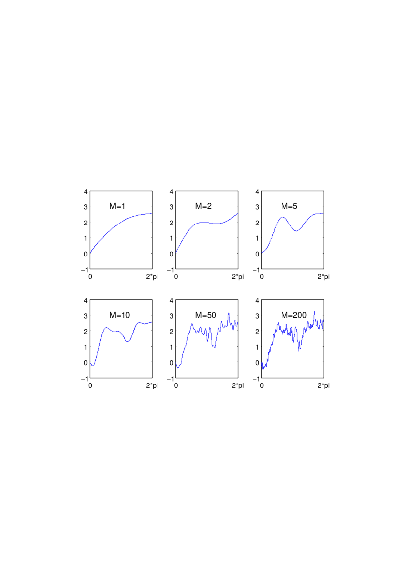
Figure 1: Paths based on the Paley-Wiener representation (8). As indicated, the six plots show the sum truncated after $M=1$, $2$, $5$, $10$, $50$ and $200$ sine terms.

Now, we may view Monte Carlo as requiring a “black box”  that returns independent samples. In our numerical SDE context, the samples come from a distribution that is only approximately correct, and the black box (the Euler–Maruyama method) comes with a dial. Turning the dial corresponds to changing $\Delta t$. Samples with a smaller $\Delta t$ are more expensive—we have to wait longer for them because the paths contain more steps. The multilevel Monte Carlo algorithm cleverly exploits this dial. The black box is used to produce samples across a range of stepsizes. Most of the samples that we ask for will be obtained quickly with relatively large $\Delta t$ values. Relatively few samples will be generated at the expensive small $\Delta t$ levels. In a sense, the large $\Delta t$ paths cover the low-frequency information so that expensive, high-frequency paths are used sparingly. Figure 1 might convince you that this idea has some merit. The next section works through the details.

5 Multilevel Monte Carlo with Euler–Maruyama

We focus now on the more general case where we wish to approximate the expected value of some function of the final time solution, $\mathbb{E}[h(X(T))]$. We have in mind the case where $X(t)$ represents an underlying asset, in risk-neutral form, and $h(\cdot)$ is the payoff of a corresponding European-style option [20, 23]. For example, $h(x)=\max(x-E,0)$ for a European call option with exercise price $E$ and expiry time $T$. For simplicity, we will consider the scalar case, so that $m=d=1$ in (1), but we note that all arguments generalise to the case of systems, with the same conclusions. We assume that the payoff function $h$ satisfies a global Lipschitz condition; this covers the call and put option cases.

Multilevel Monte Carlo uses a range of different discretization levels. At level $l$ we have a stepsize of the form

$$\Delta t_{l}=M^{-l}T,\quad\mathrm{where~{}}l=0,1,2,\ldots,L.$$ (9)

Here $M>1$ is a fixed quantity whose precise value does not affect the overall complexity of the method, in terms of the asymptotic rate as $\epsilon\to 0$. For simplicity we may think of $M=2$. As the upper limit on the level index we choose

$$L=\frac{\log\epsilon^{-1}}{\log M}.$$ (10)

In this way, at the coarsest level, $l=0$, we have the largest stepsize, $\Delta t_{0}=T$, covering the whole interval in one step. At the most refined level, $l=L$, we have $\Delta t_{L}=O(\epsilon)$—from (4), this the stepsize needed by Euler–Maruyama to achieve weak error of $O(\epsilon)$.

With each choice of stepsize, $\Delta t_{l}$, we may apply Euler–Maruyama to the SDE (1) and evaluate the payoff function $h$ at the final time. We will let the random variable $\widehat{P}_{l}$ denote this approximation to $h(X(T))$. Now, from the linearity of the expectation operator we have the telescoping sum

$$\mathbb{E}[\widehat{P}_{L}]=\mathbb{E}[\widehat{P}_{0}]+\sum_{l=1}^{L}\mathbb{E}[\widehat{P}_{l}-\widehat{P}_{l-1}].$$ (11)

In multilevel Monte Carlo, we use the expansion on the right hand side as an indirect means to evaluate the left hand side. This may be thought of as a recursive application of the control variate technique, which is widely used in applied statistics [20, 23, 37, 38]. To estimate $\mathbb{E}[\widehat{P}_{0}]$ we form the usual sample mean, based on, say, $N_{0}$, paths. This gives

$$\widehat{Y}_{0}=\frac{1}{N_{0}}\sum_{s=1}^{N_{0}}\widehat{P}_{0}^{[s]}.$$ (12)

Generally, for $\mathbb{E}[\widehat{P}_{l}-\widehat{P}_{l-1}]$ with $l>0$ we will use $N_{l}$ paths so that

$$\widehat{Y}_{l}=\frac{1}{N_{l}}\sum_{s=1}^{N_{l}}\left(\widehat{P}_{l}^{[s]}-\widehat{P}_{l-1}^{[s]}\right).$$ (13)

It is vital to point out that $\widehat{P}_{l}^{[s]}$ and $\widehat{P}_{l-1}^{[s]}$ in (13) come from the same discretized Brownian path, with different stepsizes $\Delta t_{l}$ and $\Delta t_{l-1}$, respectively. Figure 2 illustrates the idea for the case $M=2$. In words, at a general level $l$, we compute $N_{l}$ Brownian paths and, for each path, apply Euler–Maruyama twice; once with stepsize $\Delta t_{l}$ and once with stepsize $\Delta t_{l-1}$. (In practice, we compute a path at resolution $\Delta t_{l}$ and then combine Brownian increments over pairs of steps in order to get a path at resolution $\Delta t_{l-1}$.) Having constructed our $N_{l}$ independent paths for level $l$, we start afresh at level $l+1$; none of the earlier information is re-used and new (independent) pseudo-random numbers are generated.

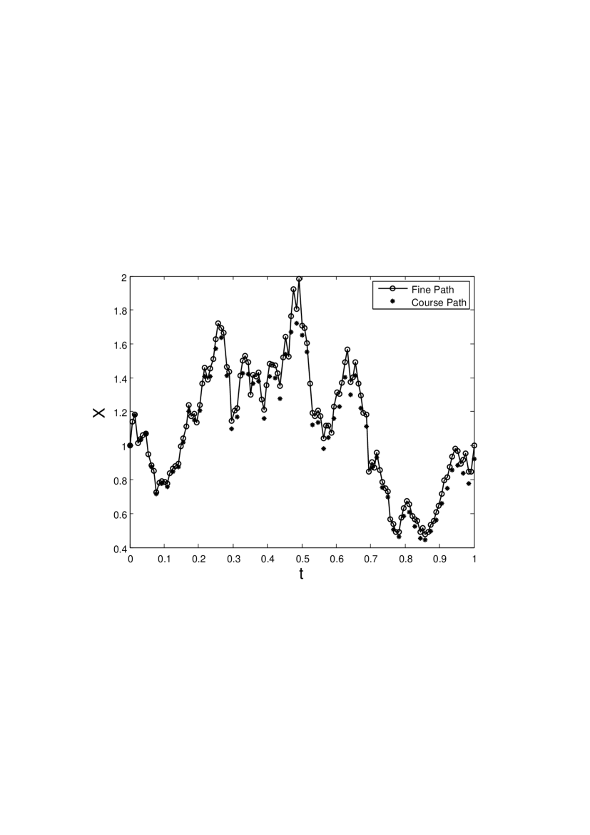
Figure 2: Illustration of how the estimator $\widehat{Y}_{l}$ in (13) is constructed. Circles (joined by straight lines for clarity) show the refined Euler–Maruyama path, with stepsize $\Delta t=2^{-l}T$. Asterisks show the coarser Euler–Maruyama path, with stepsize $\Delta t=2^{-l+1}T$, computed with the same Brownian increments.

Because of the choice of $L$ in (10) we know from (11) that our estimator will have the required $O(\epsilon)$ bias. Now we will see how to choose the values of $\{N_{l}\}_{l=0}^{L}$ to achieve the corresponding accuracy in the overall confidence interval.

Considering a general level where $l>0$, appealing to the strong convergence behaviour (6) of Euler–Maruyama and our assumption that $h$ is globally Lipschitz, we have

$$\mathsf{var}[\widehat{P}_{l}-h(X(T))] = \mathbb{E}[(\widehat{P}_{l}-h(X(T)))^{2}]-(\mathbb{E}[\widehat{P}_{l}-h(X(T))])^{2}$$ (14)

$$\leq \mathbb{E}[(\widehat{P}_{l}-h(X(T)))^{2}]$$ (15)

$$\leq \mathrm{constant}\times\mathbb{E}[(X_{N}-X(T))^{2}]$$ (16)

$$= O(\Delta t_{l}).$$ (17)

It then follows from Minkowski’s Inequality [8] that

$$\mathsf{var}[\widehat{P}_{l}-\widehat{P}_{l-1}] = \mathsf{var}[\widehat{P}_{l}-h(X(T))+h(X(T))-\widehat{P}_{l-1}]$$ (18)

$$\leq \left(\sqrt{\mathsf{var}[\widehat{P}_{l}-h(X(T))]}+\sqrt{\mathsf{var}[h(X(T))-\widehat{P}_{l-1}]}\right)^{2}$$

$$= O(\Delta t_{l}).$$

Applying this result in (13) we conclude that $\widehat{Y}_{l}$ has a variance of $O(\Delta t_{l}/N_{l})$ for $l>1$. Because all levels are independent, we deduce that

$$\mathsf{var}\left[\widehat{Y}_{0}+\sum_{l=1}^{L}\widehat{Y}_{l}\right]=\mathsf{var}[\widehat{Y}_{0}]+\sum_{l=1}^{L}O(\Delta t_{l}/N_{l}).$$

To balance the variance evenly across levels $l=1,2,\ldots,L$ and to control the variance at level $l=0$, we choose $N_{l}=O(\epsilon^{-2}L\Delta t_{l})$. It then follows that our overall estimator has variance

$$O(\epsilon^{2})+\sum_{l=1}^{L}O(\epsilon^{2}/L)=O(\epsilon^{2}).$$

In this way, we have achieved the bias and variance required to give a confidence interval of the specified $\epsilon$ level of accuracy.

To quantify how the complexity of this algorithm scales with $\epsilon$, we sum the cost of level $l$ from $l=0$ to $L$ to give

$$\sum_{l=0}^{L}N_{l}\Delta t_{l}^{-1}=\sum_{l=0}^{L}\epsilon^{-2}L\Delta t_{l}\Delta t_{l}^{-1}=L^{2}\epsilon^{-2}.$$

From (10) this expression becomes $O(\epsilon^{-2}\left(\log\epsilon\right)^{2})$, as we quoted in section 3.

At this stage, a few remarks are in order:

Constructive Upper Bound:

In the course of the analysis above, we came up with a general-purpose choice for the number of paths at each level, $\{N_{l}\}_{l=0}^{L}$. The final complexity count is therefore an upper bound on the best possible value. In practice, for a given problem and accuracy requirement, we can perform a cheap pre-processing step where appropriate variances are estimated and an optimization problem is solved in order to give a sequence $\{N_{l}\}_{l=0}^{L}$; see, for example, [18].

Weak versus Strong:

The key inequality (18), which guarantees tight coupling between coarse and fine paths, made use of the strong convergence property. For small $\Delta t_{l}$, both paths are close to the true path, so the paths must be close to each other. In this sense, both strong and weak error rates are key ingredients in the analysis. We note, however, that Giles [13] has also developed estimators that do not rely directly on strong convergence.

Variance and Second Moment

In deriving the inequality (17), we discarded the square of the first moment and used the second moment as an upper bound for the variance. This may appear to be a very crude step, but in our context it does not degrade the final conclusion. (In a different, Poisson-driven setting where a multilevel method was developed and analysed, the step (14)–(15) is no longer optimal—it is beneficial to analyse the variance directly [3].)

Exploiting Structure:

As mentioned above, multilevel Monte Carlo may be viewed as a recursive version of the control variate approach. In the simplest version of control variates, if we wish to compute $\mathbb{E}[X]$, we may instead compute $\mathbb{E}[X-Y]$ and add $\mathbb{E}[Y]$, where $Y$ is a suitably constructed random variable such that $X-Y$ has small variance and $\mathbb{E}[Y]$ is readily available [20, 23]. However, the success of this technique usually relies on incorporating some extra knowledge of the problem: a structure such as symmetry or convexity, or the existence of a “nearby”  problem that is analytically tractable. In this respect, the multilevel Monte Carlo method for SDEs is very different from traditional control variates: the analysis is completely general and no special insights are needed about the nature of the underlying SDE, other than knowledge of the basic weak and strong convergence properties.

Multilevel versus Multigrid:

In [16], Giles explains that the multigrid approach in numerical PDEs was “the inspiration for the author in developing the MLMC method for SDE path simulation.” There are clear similarities between the two: the use of geometrically refined/coarsened grids and the idea that relatively little work needs to be expended on the fine grids in order to resolve high frequency components. However, it is important to keep in mind that there are also conceptual differences between the two techniques: multilevel Monte Carlo is distinct, and novel. For example, multilevel Monte Carlo does not involve the notion of passing information up and down the refinement levels, as is done with multigrid V or W cycles.

Related Earlier Methods:

As discussed in [16, section 1.3], related earlier work on improving Monte Carlo when samples are generated via discretization was performed by Heinrich, see, for example [21, 22], and Kebaier [29] devised a two-level approach to path simulation.

Based on the type of analysis that we summarized above, it is possible to state a general theorem about multilevel simulation:

Theorem 5.1 (Giles; see for example, [16])

Let $P$ denote a random variable, and let $P_{l}$ denote the corresponding level $l$ numerical approximation. If there exist independent estimators $Y_{l}$ based on $N_{l}$ Monte Carlo samples, and positive constants $\alpha,\beta,\gamma,c_{1},c_{2},c_{3}$ such that $\alpha\geq{\scriptstyle{{\frac{1}{2}}}}\min(\beta,\gamma)$ and

1. $|\mathbb{E}[P_{l}-P]|\leq c_{1}2^{-\alpha l}$

2. $\mathbb{E}[Y_{0}]=\mathbb{E}[P_{0}]$ and  $\mathbb{E}[Y_{l}]=\mathbb{E}[P_{l}-P_{l-1}]$ for $l>0$

3. $\mathsf{var}[Y_{l}]\leq c_{2}N_{l}^{-1}2^{-\beta l}$

4. $\mathbb{E}[C_{l}]\leq c_{3}N_{l}2^{\gamma l}$, where $C_{l}$ is the computational complexity of $Y_{l}$

then there exists a positive constant $c_{4}$ such that for any $\epsilon<e^{-1}$ there are values $L$ and $N_{l}$ for which the multilevel estimator

$$Y=\sum_{l=0}^{L}Y_{l}$$

has a mean-square error with bound

$$\mathbb{E}\left[(Y-\mathbb{E}[P])^{2}\right]<\epsilon^{2}$$

with a computational complexity $C$ with bound

$$\mathbb{E}[C]\leq\left\{\begin{array}[]{ll}c_{4}\epsilon^{-2},&\beta>\gamma\\ c_{4}\epsilon^{-2}(\log(\epsilon))^{2},&\beta=\gamma\\ c_{4}\epsilon^{-2-(\gamma-\beta)/\alpha},&\beta<\gamma.\end{array}\right.$$

Giles [13] has also shown how to construct estimators for which $\beta>\gamma=1$, by replacing Euler–Maruyama with the more strongly accurate Milstein scheme. For European-style options with Lipschitz payoff functions, this makes $O(\epsilon^{-2})$ complexity achievable. From the arguments in section (3), it is intuitively reasonable that this is the optimal rate. The issue is formalized in [35], and optimality is confirmed.

In section 2 we mentioned that the basic Euler–Maruyama method (1) may fail to converge in a weak or strong sense on nonlinear SDEs in the asymptotic limit $\Delta t\to 0$. A closely related question, of direct relevance to this review, is whether the combination of “Euler–Maruyama plus Monte Carlo” converges in the $\epsilon\to 0$ limit. In [25, 26], Hutzenthaler and Jentzen showed that Euler–Maruyama Monte Carlo can achieve convergence in a $\mathbb{P}$-almost sure sense in cases where the underlying Euler–Maruyama scheme diverges. This can happen when the events causing Euler–Maruyama to diverge are so rare that they are extremely unlikely to impact on any of the Monte Carlo samples. However, in [28] Hutzenthaler, Jentzen and Platen showed that the multilevel Monte Carlo method does not inherit this property. They established this result using a counterexample of the form

$$dX(t)=-X(t)^{5}dt,$$ (19)

with $X(0)$ having a standard Gaussian distribution, where $\mathbb{E}[X(t)^{2}]$ is the required moment. Note that the SDE (19) has a zero drift term, so it may also be regarded as a random ODE. A modified version of Euler–Maruyama, known as a tamed method, was shown in [28] to recover convergence in the multilevel setting.

6 Computational Experiments

Asymptotic, $\epsilon\to 0$, analysis indicates that multilevel Monte Carlo offers a dramatic improvement in computational complexity. Numerous computational studies have confirmed that this potential can be realised in practice.

Giles has made MATLAB code available at

Ψhttp://people.maths.ox.ac.uk/gilesm/acta/
Ψ

that can be used as the basis for computational experimentation. In Figure 3 we show results based on this code. Here, we have an asset model given by geometric Brownian motion

$$dX(t)=0.05X(t)dt+0.25X(t)dW(t),\quad X(0)=100.$$

We consider (a) a European call and (b) a digital call option over $[0,T]$ with $T=1$ and exercise price $100$. So the payoff functions, after discounting for interest, are

$$h(x)=e^{-0.05T}\max(x-100,0)$$

for the call option and

$$h(x)=\left\{\begin{array}[]{ll}e^{-0.05T}100&\mathrm{~{}when~{}}x>100\\ 0&\mathrm{~{}when~{}}x<100\end{array}\right.$$

for the digital option. (For those who worry about probability zero events, the code defines $h(100)=e^{-0.05T}(100+0)/2$.) The code repeats the Monte Carlo simulation for accuracy requests of $\epsilon=0.1,0.05,0.02,0.01,0.005$. The upper left picture in Figure 3 shows, for the call option, the number of paths $N_{l}$ used at each level $l$ in the multilevel method. We see that for a given $\epsilon$ more paths are used at the cheaper (small $l$) levels, and as $\epsilon$ is decreased, so that more accuracy is required, extra levels are added. The upper right picture indicates the corresponding computational cost in terms of run time. More precisely, the asterisks (joined by dashed lines) show the cost weighted by $\epsilon^{2}$ as a function of $\epsilon$. We see that this quantity remains approximately constant, as predicted by the analysis. The picture also shows the scaled cost for an equivalent standard Monte Carlo computation, using a solid linetype. We see a much larger cost that appears to grow faster than $\epsilon^{-2}$. The lower pictures in Figure 3 give the same results for the case of the digital option, and again the multilevel version is seen to be more efficient than standard Monte Carlo.

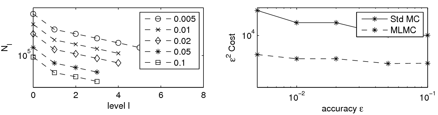
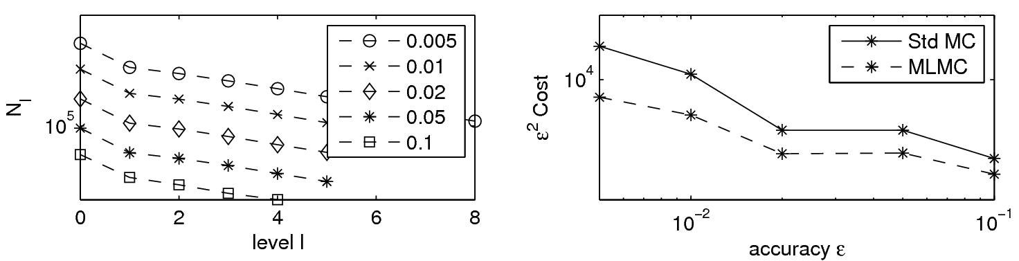
Figure 3: Output from the multilevel Monte Carlo code made available by Giles (see text for web site address). Left hand pictures show the number of paths per level at each target accuracy. Right hand pictures show the computation time, scaled by $\epsilon^{2}$. Upper pictures are for a European call option. Upper pictures are for a digital option.

7 Follow-on Research

In this section we summarize some of the key advances that have been made since the original multilevel breakthrough [14]. We focus on work that is directly relevant to financial option valuation. The comprehensive overviews [16, 18] can be consulted for further details on these, and other, areas. The webpage maintained by Giles at

http://people.maths.ox.ac.uk/~gilesm/mlmc_community.html

is also an excellent source of up-to-date information.

7.1 Beyond European Calls and Puts

A key step in the analysis of section 5 was to show that the coarse and refined paths are tightly coupled, in the sense that they produce payoffs whose difference has small variance. The logic behind the analysis may be loosely summarized as

A

strong convergence of Euler–Maruyama $\Rightarrow$

B

coarse and refined paths close to the true path $\Rightarrow$

C

coarse and refined paths close to each other $\Rightarrow$

D

coarse and refined payoffs close to each other.

The C $\Rightarrow$ D step appealed to the global Lipschitz property of $h$. This is valid for European call and put options, where $h(x)=\max(x-E,0)$ and $h(x)=\max(E-x,0)$, respectively. However, the analysis must be refined for those European-style options where $\mathbb{E}[h(X(T))]$ is required for functions $h$ that violate the global Lipschitz criterion. We may also wish to deal with path-dependent options where an expected value operation is applied to a functional depending on some or all of the values $X(t)$ for $0\leq t\leq T$.

These more exotic options include problematic classes where, for certain SDE paths, the payoff may be very sensitive to small changes. For example, with digital options that expire close to the money, a small change in the asset path can lead to an $O(1)$ change in the payoff. Similarly, the payoff from a barrier option is very sensitive to those paths that flirt with the barrier. In these cases, the logical flow above above must be adapted. Intuitively, we should be able to exploit the fact that troublesome paths are the exception rather than the rule, and hence C $\Rightarrow$ D with high probability. In some cases this allows us to recover the computational complexity that we saw for European calls and puts. In other cases we must accept a slight increase in cost.

The behaviour of multilevel Monte Carlo for Asian, lookback and digital options was considered computationally in the original work of Giles [14]. Rigorous analysis to back up these results for barrier, lookback and digital options was first given in [17]. Further work has been targeted at binary options [5], Asian options [2], basket options [15], barrier options [10] and American options [6]. The use of multilevel Monte Carlo to compute sensitivities with respect to problem parameters, that is, Greeks, was considered in [7].

7.2 Further Developments

It is common practice to combine more than one variance reduction technique. Given that antithetic variables can be effective in option valuation [20, 23], it is natural to consider embedding this approach within the multilevel framework. Giles and Szpruch [11, 19] have shown that this can be effective, particularly when Milstein is used for the numerical integration. A conditional Monte Carlo approach has also been shown to be fruitful in the mutlilevel setting [13]. In a different direction, Rhee and Glynn [36] have proposed an extra level of randomization that produces an unbiased multilevel estimator.

To go beyond the asymptotic $O(\epsilon^{-2})$ complexity barrier it is possible to move to quasi Monte Carlo, where a low-discrepancy sequence replaces a pseudo-random sequence. Giles and Waterhouse [12] have demonstrated that a combination of quasi Monte Carlo and multilevel can outperform each separate technique.

Finally, we note that the multilevel methodology has also been extended to asset models that are not driven purely by Brownian motion [9, 40].

8 Discussion

Our aim in this article was to explain in an accessible manner the key ideas behind the multilevel Monte Carlo method. We focussed on the case of SDE-based financial option valuation, where Monte Carlo is a widely used tool. At the heart of the technique is a very general and widely applicable philosophy—a recursive application of control variates that relies on tight coupling between simulations at different resolutions. The resulting algorithm is sufficiently simple and effective that it can be implemented straightforwardly and used to produce noticable gains in computational efficiency in very general circumstances. However, as evidenced by the wealth of current research activity, there is also substantial scope for (a) refining the multilevel approach in order to exploit problem-specific information and (b) developing multilevel methods in many other stochastic simulation scenarios. For these reasons we envisage multilevel Monte Carlo evolving into a cornerstone of computational finance.

Acknowledgement The author is funded by a Royal Society/Wolfson Research Merit Award and an EPSRC Digital Economy Fellowship. He is grateful to Mike Giles for creating and placing in the public domain the code that was used as the basis for Figure 3.

References

- [1] Y. Ait-Sahalia, Testing continuous-time models of the spot interest rate, Review of Financial Studies, (1999), pp. 385–426.
- [2] M. B. Alaya and A. Kebaier, Multilevel Monte Carlo for Asian options and limit theorems, Monte Carlo Methods and Applications, 20 (2014), pp. 181–194.
- [3] D. F. Anderson, D. J. Higham, and Y. Sun, Complexity of multilevel Monte Carlo tau-leaping, SIAM Journal on Numerical Analysis, 52 (2015), pp. 3106–3127.
- [4] D. F. Anderson and J. C. Mattingly, A weak trapezoidal method for a class of stochastic differential equations, Communications in Mathematical Sciences, 9 (2011), pp. 301–318.
- [5] R. Avikainen, Convergence rates for approximations of functionals of SDEs, 13 (2009), pp. 381 –401.
- [6] D. Belomestny, J. Schoenmakers, and F. Dickmann, Multilevel dual approach for pricing American style derivatives, Finance and Stochastics, 17 (2013), pp. 717–742.
- [7] S. Burgos and M. B. Giles, Computing Greeks using multilevel path simulation, in Monte Carlo and Quasi Monte Carlo Methods 2010, L. Plaskota and H. Wozniakowski, eds., Springer, 2012, pp. 281–296.
- [8] M. Capiński and E. Kopp, Measure, Integral and Probability, Springer, Berlin, 1999.
- [9] S. Dereich and F. Heidenreich, A multilevel Monte Carlo algorithm for Lévy-driven stochastic differential equations, Stochastic Processes and their Applications, (2011), pp. 1565–1587.
- [10] M. Giles, K. Debrabant, and A. Rößler, Numerical analysis of multilevel Monte Carlo path simulation using the Milstein discretisation, ArXiv preprint: 1302.4676, (2013).
- [11] M. Giles and L. Szpruch, Antithetic multilevel Monte Carlo estimation for multidimensional SDEs, in Monte Carlo and Quasi-Monte Carlo Methods 2012, J. Dick, F. Kuo, G. Peters, and I. Sloan, eds., Springer, 2013, pp. 367–384.
- [12] M. Giles and B. Waterhouse, Multilevel quasi-Monte Carlo path simulation, in Advanced Financial Modelling, Radon Series on Computational and Applied Mathematics, De Gruyter, 2009, pp. 165–181.
- [13] M. B. Giles, Improved multilevel Monte Carlo convergence using the Milstein scheme, in Monte Carlo and Quasi-Monte Carlo Methods, Springer, 2007, pp. 343–358.
- [14] , Multilevel Monte Carlo path simulation, Operations Research, 56 (2008), pp. 607–617.
- [15] , Multilevel Monte Carlo for basket options, in Proceedings of the 2009 Winter Simulation Conference, Austin, M. D. Rossetti, R. R. Hill, B. Johansson, A. Dunkin, and R. G. Ingalls, eds., IEEE, 2009, pp. 1283–1290.
- [16] , Multilevel Monte Carlo methods, in Monte Carlo and Quasi Monte Carlo Methods 2012, J. Dick, F. Y. Kuo, G. W. Peters, and I. H. Sloan, eds., Springer, 2014, pp. 79–98.
- [17] M. B. Giles, D. J. Higham, and X. Mao, Analysing multi-level Monte Carlo for options with non-globally Lipschitz payoff, Finance and Stochastics, 13 (2009), pp. 403–413.
- [18] M. B. Giles and L. Szpruch, Multilevel Monte Carlo methods for applications in finance, in Recent Developments in Computational Finance, T. Gerstner and P. E. Kloeden, eds., World Scientific, 2013.
- [19] , Antithetic multilevel Monte Carlo estimation for multi-dimensional SDEs without Lévy area simulation, Annals of Applied Probability, 24 (2014), pp. 15850–1620.
- [20] P. Glasserman, Monte Carlo Methods in Financial Engineering, Springer, Berlin, 2004.
- [21] S. Heinrich, Monte Carlo complexity of global solution of integral equations, Journal of Complexity, 14 (1998), pp. 151–175.
- [22] , Monte Carlo approximation of weakly singular integral operators, Journal of Complexity, 22 (2006), pp. 192–219.
- [23] D. J. Higham, An Introduction to Financial Option Valuation: Mathematics, Stochastics and Computation, Cambridge University Press, Cambridge, 2004.
- [24] D. J. Higham, X. Mao, and A. M. Stuart, Strong convergence of Euler-type methods for nonlinear stochastic differential equations, SIAM J. Num Anal., 40 (2002), pp. 1041–1063.
- [25] M. Hutzenthaler and A. Jentzen, Convergence of the stochastic Euler scheme for locally Lipschitz coefficients, Found. Comput. Math., 11 (2011), pp. 657–706.
- [26] , Numerical approximations of stochastic differential equations with non-globally Lipschitz continuous coefficients, Memoirs of the American Mathematical Society, 236 (2014), p. in press.
- [27] M. Hutzenthaler, A. Jentzen, and P. E. Kloeden, Strong and weak divergence in finite time of Euler’s method for stochastic differential equations with non-globally Lipschitz continuous coefficients, Proc. R. Soc. A, 467 (2011), pp. 1563–1576.
- [28] M. Hutzenthaler, A. Jentzen, and P. E. Kloeden, Divergence of the multilevel Monte Carlo Euler method for nonlinear stochastic differential equations, Annals of Applied Probability, 23 (2013), pp. 1913–1966.
- [29] A. Kebaier, Statistical Romberg extrapolation: a new variance reduction method and applications to option pricing, Annals of Applied Probabilty, 14 (2005), pp. 2681–2705.
- [30] P. E. Kloeden and A. Neuenkirch, The pathwise convergence of approximation schemes for stochastic differential equations, London Mathematical Society, 10 (2007), pp. 235–253.
- [31] P. E. Kloeden and E. Platen, Numerical Solution of Stochastic Differential Equations, Springer Verlag, Berlin, Third Printing, 1999.
- [32] T. Mikosch, Elementary Stochastic Calculus (with Finance in View), World Scientific, Singapore, 1998.
- [33] G. N. Milstein and M. V. Tretyakov, Stochastic Numerics for Mathematical Physics, Springer-Verlag, Berlin, 2004.
- [34] G. N. Milstein and M. V. Tretyakov, Numerical integration of stochastic differential equations with nonglobally Lipschitz coefficients, SIAM J. Numer. Anal., 43 (2005), pp. 1139–1154.
- [35] T. Müller-Gronbach and K. Ritter, Variable subspace sampling and multi-level algorithms, in Monte Carlo and Quasi-Monte Carlo Methods 2008, P. L’Ecuyer and A. Owen, eds., Springer, 2009, pp. 131–156.
- [36] C. Rhee and P. W. Glynn, A new approach to unbiased estimation for SDE’s, in Proceedings of the 2012 Winter Simulation Conference, C. Laroque, J. Himmelspach, R. Pasupathy, O. Rose, and A. Uhrmacher, eds., 2012, pp. 201–207.
- [37] C. P. Robert and G. Casella, Monte Carlo Statistical Methods, Springer, Berlin, 2nd ed., 2004.
- [38] R. Seydel, Tools for Computational Finance, Springer, Berlin, fifth ed., 2012.
- [39] L. Szpruch, X. Mao, D. J. Higham, and J. Pan, Strongly nonlinear Ait-Sahalia-type interest rate model and its numerical approximation, BIT Numerical Mathematics, 51 (2011), pp. 405–425.
- [40] Y. Xia and M. B. Giles, Multilevel path simulation for jump-diffusion SDEs, in Monte Carlo and Quasi Monte Carlo Methods 2010, L. Plaskota and H. Wozniakowski, eds., Springer, 2012, pp. 695–708.