Large deviations, condensation, and giant response in a statistical system

Abstract

We study the probability distribution $P$ of the sum of a large number of non-identically distributed random variables $n_{m}$. Condensation of fluctuations, the phenomenon whereby one of such variables provides a macroscopic contribution to the global probability, is discussed and interpreted in analogy to phase-transitions in Statistical Mechanics. A general expression for $P$ is derived, and its sensitivity to the details of the distribution of a single $n_{m}$ is worked out. These general results are verified by the analytical and numerical solution of some specific examples.

I Introduction

Condensation is the phenomenon whereby a finite fraction of some quantity, e.g. a particle density, concentrates into a small region of phase-space, as in the paradigmatic example of a vapor transforming into a liquid when crossing a phase-transition. Condensation is observed in a number of different models, related to magnetic properties condzrp1 , gravity bialas1 ; bialas2 ; bialas3 , mass transport and other issues condzrp2 ; condzrp3 ; condzrp4 ; condzrp5 ; condzrp6 ; condzrp7 ; condzrp7a ; condzrp7b ; condzrp7c ; condzrp7d ; condzrp8 ; condzrp9 ; god1 ; god2 ; god3 ; god4 . Despite the prominent role played by molecular interactions in most cases, condensation can also be observed in non-interacting systems as, for instance, in a quantum Bose-Einstein condensate bec or in classical models such as the spherical model of a ferromagnet condzrp2 . In the above mentioned cases condensation occurs because the condensing quantity – the particle number in the former example or the spin variance in the latter – is conserved. This constraint acts like an effective interaction among the constituents bringing about the transition effint1 ; effint2 . Indeed, condensation does not occur in a non-interacting boson gas – as in the case of photons – which does not conserve the number of constituents.

A different manifestation of condensation is observed when probability distributions of a fluctuating collective variable ${\cal N}$, such as the number of particles in a thermodynamic system, are considered. In this case, a fluctuation ${\cal N}=N$ well above the typical value can be associated to a condensed configuration of the system effint1 ; effint2 ; condfluc1 ; condfluc2 ; condfluc3 ; condfluc4 ; condfluc5 ; condfluc6 ; condfluc7 ; condfluc8 ; mars . This phenomenon, referred to as condensation of fluctuations, is not restricted to the particle number ${\cal N}$ but was observed for quantities as diverse as energy, exchanged heats, particles currents etc… effint1 ; effint2 ; condfluc1 ; condfluc2 ; condfluc3 ; condfluc4 ; condfluc5 ; condfluc6 ; condfluc7 ; condfluc8 ; mars . It was shown effint1 ; effint2 that in some systems condensation of fluctuations may occur because, from the mathematical point of view, asking for a specific value ${\cal N}=N$ constraints the system similarly to what a conservation law does.

In this paper we study the probability distribution $P$ of the sum ${\cal N}$ of $M$ non-identically distributed random variables. We discuss how an interpretation can be provided, along the guidelines of Statistical Mechanics, in terms of a phase-transition between a normal phase with a vanishing order parameter $\rho_{\ell}$ and a condensed one with $\rho_{\ell}>0$. A general expression for the probability $P$ is found and the radically different behavior of this quantity in the normal and in the condensed phase are discussed and illustrated by comparing the analytical and numerical solution of some specific models. In particular, in the condensed phase, the notable phenomenon of the giant response – a dramatic change of $P$ as the statistical properties of even a single random variable is modified – is pointed out.

This paper is organized as follows: In Sec. II we introduce the statistical model that will be studied and set the notation. In Secs. III and IV its behavior is discussed when condensation does not occur and when it does, providing also an example by means of an analytically tractable case for identically distributed variables (Secs. III.1 and IV.1, respectively). In Sec. V the case of non identically distributed variables is addressed and the phenomenon of the giant response is discussed (Sec. V.1). Some examples are considered in Sec. V.2. Finally, In Sec. VI we briefly summarize and conclude the paper.

II The statistical model

In order to set the stage, let us consider the independent variables $n_{m}$ ($m=1,M$) subject to a probability $p_{m}(n_{m};K)$, where $K$ is a set of parameters. This probabilistic setup is suited to describe at a simple level a variety of systems ranging from physics to chemistry, biology and social sciences. For instance, one can consider $M$ receptors where $n_{m}$ ligand particles, like those of a pollutant, can be adsorbed, or $n_{m}$ electrons populating $M$ atomic levels. One can also think of $M$ individuals, or agents, collecting $n_{m}$ resources with a certain probability $p_{m}$. In the former examples the temperature can be one of the control parameters $K$ but, in general, others can be present.

We fix the language by speaking of $M$ receptors hosting a total number

$${\cal N}=\sum_{m=1}^{M}n_{m}$$ (1)

of particles, with an average value $\langle{\cal N}\rangle=\sum_{m=1}^{M}\langle n_{m}\rangle$, where $\langle n_{m}\rangle=\sum_{n}n\,p_{m}(n;K)$. For ease of notation the dependence on $K$ will be often dropped, and $M$ will be considered large.

We are interested in the probability to observe a total number ${\cal N}=N$ of particles

$$P(N,M) = \sum_{n_{1},n_{2},\dots,n_{M}}p_{1}(n_{1})p_{2}(n_{2})\cdots p_{M}(n_{M})\,\delta_{{\cal N},N}=$$ (2)

$$= \frac{1}{2\pi i}\oint dz\,e^{M[\ln Q(z,M)-\rho\ln z]},$$

where, for discrete variables, we used the representation $\delta_{{\cal N},N}=\frac{1}{2\pi i}\oint dz\,z^{-(N-{\cal N}+1)}$, with

$$Q(z,M)=\left[\prod_{m=1}^{M}\sum_{n_{m}}p_{m}(n_{m})z^{n_{m}}\right]^{\frac{1}{M}}$$ (3)

and $\rho=\frac{N-1}{M}\simeq\frac{N}{M}$ is the particles density.

As explained in condzrp4 ; effint1 ; effint2 the probability distribution $P$ of the fluctuations of the particle number corresponds also to the partition function of a dual model where the number of particles is conserved. For example, with some particular choices of the microscopic probabilities $p$ that will be considered below, such dual model corresponds to specific instances of the so called urn model (or balls in boxes model) or of a zero-range process. This duality, which to the best of our knowledge was never discussed in connection to the above mentioned models, allows us to borrow a number of well established results in this research areas to illustrate the behavior of $P$ – whose properties are here discussed in a rather large generality – in some exemplifying cases.

The following relation holds condzrp3 ; bialas3

$$P(N,M)=\sum_{n=0}^{N}\pi(n,N,M)$$ (4)

where

$$\pi(n,N,M)=P(N-n,M-1)\,p_{M}(n)$$ (5)

is the probability that, when the $M$-th receptor is added to the previous $M-1$, $n$ particles are stored in it. eq. (4) is a recurrence relation allowing one to determine the probability distribution of $M$ variables once the one for $M-1$ is known.

Let us discuss the basic mechanisms whereby the recurrence (4) works to build up the full probability $P(N,M)$. Denoting with $\overline{N}=M\overline{\rho}$ the value of $N$ where $P$ is maximum, the largest $P(N-n,M-1)$ in eq. (5) is the one with $n=N-\overline{N}$. Notice that this term is present in eq. (4) only if $N\geq\overline{N}$.

III Gas phase

According to the previous discussion, for $N\leq\overline{N}$, $\pi$ has a maximum at a value $n=n_{g}$ which is microscopic and does not scale with $M$ (see the inset of fig.1 for a specific example with $n_{g}=0$, to be discussed below). This is so because the quantities $P(N-n,M-1)$ in eq. (5) lower with $n$ (i.e. moving away from the maximum) and the same is true for $p_{M}(n)$, for sufficiently large $n>n_{g}$ (being $p_{M}(n)$ normalized). If the $p_{m}$’s are monotonously decreasing, it is $n_{g}=0$.

A similar setting, with $\pi$ peaked at a microscopic $n_{g}$, is found also for $N>\overline{N}$, when the largest probability $P(\overline{N},M-1)$ is contained in the sum on the r.h.s. of eq. (4), but its maximum is tamed by the microscopic probabilities, i.e. $\lim_{M\to\infty}P(\overline{N},M-1)p_{M}(N-\overline{N})=0$.

The situation with $\pi$ peaked in $n=n_{g}$ is physically intuitive: It expresses the fact that, when $M$ is large, the occupancy $\pi$ of the new receptor (the $M$-th) is microscopic. We will denote this situation, with a uniformly small occupation, the normal (or gas) phase.

III.1 An example

Let us illustrate these behaviors by considering a specific example with power-law distribution

$$p_{m}(n)=c\,(n+1)^{-K_{m}},$$ (6)

where $K_{m}>1$ and $c$ is a normalization.

We start with the simplest case where $K_{m}\equiv K$ does not depend on $m$ mars . In the inset of fig.1, $\pi$ is plotted for $K=3/2$ and different choices of $N$. Here one observes a sharp peak in $n=n_{g}\equiv 0$, as expected.

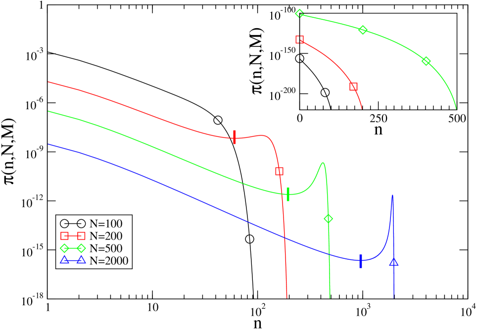
Figure 1: The quantity $\pi(n,N,M)$ is plotted against $n$ for the model with probabilities (6) with a uniform $K_{m}=K=3>K_{c}$, for $M=246$ and the values of $N$ indicated in the key. The location of $n_{gl}$ is indicated with a bold vertical segment. In the inset the same plot is made for $K_{m}=K=3/2<K_{c}$.

In the gas phase, $P$ can be determined in the large-$M$ limit by a steepest-descent evaluation bialas1 ; bialas2 ; god1 ; god2 ; god3 ; god4 ; condzrp3 ; effint1 ; effint2 ; mars ; touch of the integral on the r.h.s. of eq. (2), leading to

$$P(N,M)\simeq e^{-MR(\rho)},$$ (7)

with an $M$-independent rate-function

$$R(\rho)=-\ln Q[z^{*}(\rho)]+\rho\ln z^{*}(\rho),$$ (8)

where $z^{*}(\rho)$ is given by the saddle-point equation

$$z^{*}(\rho)\,\frac{Q^{\prime}[z^{*}(\rho)]}{Q[z^{*}(\rho)]}=\rho.$$ (9)

For the specific example above, this equation can be cast as

$$\frac{Li_{K-1}(z^{*})}{Li_{K}(z^{*})}=\rho+1,$$ (10)

where $Li_{K}(z)$ is the polylogarithm (Jonquière’s function). It admits a solution with $z<1$ for any finite value of $\rho$ if $K\leq K_{c}=2$ condzrp3 ; condzrp7c ; bialas1 ; bialas2 ; bialas3 ; god1 ; god2 ; god3 ; god4 . $P$ is then expressed by Eqs. (7,8) with condzrp3 ; bialas1 ; bialas2 ; bialas3 ; god1 ; god2 ; god3 ; god4

$$Q(z^{*})=Li_{K}(z^{*}).$$ (11)

The rate-function $R(\rho)$ obtained in this way is plotted with a black heavy dashed line in fig.2. In the same picture the quantity

$${\cal R}(\rho,M)=-\frac{1}{M}\ln P(M\rho,M)$$ (12)

obtained from eq. (2) by exact enumeration, is shown for different choices of $M$. One observes that ${\cal R}$ approaches the asymptotic $M$-independent form $R(\rho)$ as $M$ is increased. Notice that the convergence is faster at small densities. It must be recalled that, for $K\leq K_{c}$, the average number $\langle N\rangle$ of particles is not finite, meaning that in the large-$M$ limit fluctuations with large $N$ are very likely, as it is reflected by the vanishing of $R(\rho)$ at large densities. However, for finite $M$ such large values of $N$ cannot be sustained and ${\cal R}$, after reaching a minimum, raises again increasing $\rho$, thus determining the existence of a most probable value of the fluctuations. The position of such value is pushed to larger densities by increasing $M$, providing in this way a gradual convergence, from smaller to larger values of $\rho$, of ${\cal R}$ towards $R$.

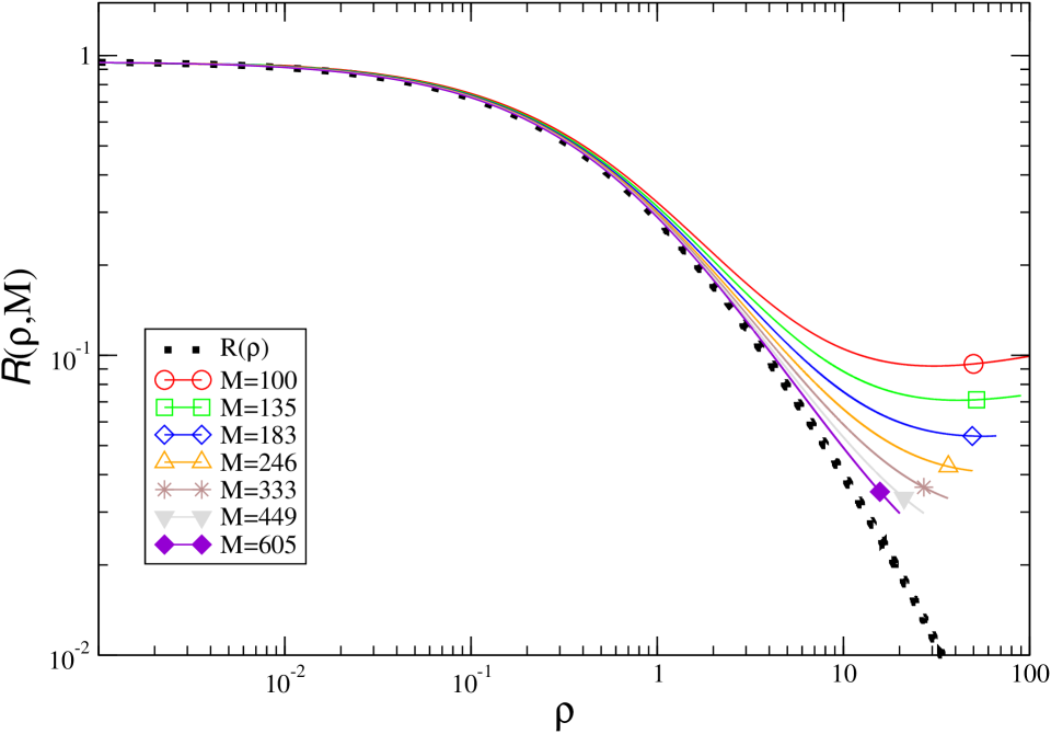
Figure 2: ${\cal R}(\rho,M)$ is plotted against $\rho$ for for the model with probabilities (6) with a uniform $K_{m}=K=3/2<K_{c}$, for different values of $M$ in the key. The heavy dashed line is the asymptotic (for $M\to\infty$) expression $R(\rho)$ obtained from Eqs. (8,10,11).

IV Condensed phase

A radically different situation occurs for $N>\overline{N}$, when $P(\overline{N},M-1)$ grows fast enough to give $\lim_{M\to\infty}P(\overline{N},M-1)p_{M}(N-\overline{N})\neq 0$. For the choice (6) with $K_{m}=K$, this happens when $K>K_{c}$.

In this case the sum in eq. (4) does not only take contributions around the microscopic value $n_{g}$, since $\pi$ can be non-negligible up to a certain $n=n_{\ell}$ of order $M$. This is because $\pi$ is triggered by the maximum of $P(N-n,M-1)$ at a value $n=N-\overline{N}$ which, for given $\rho$, is of order $M$ itself. Usually $P$ is sharply peaked around the maximum as to give $n_{\ell}\simeq N-\overline{N}$ for $N$ sufficiently larger than $\overline{N}$. Fig.1 shows this for the model (6) with $K=3$: $\pi$ develops a second peak at $n=n_{\ell}\simeq N-\overline{N}$ and only for $n>n_{\ell}$ it drops down to negligible values. The properties of this second peak can be described using extreme-value statistics evansmaj .

The physical interpretation is that, when a value of $N$ larger than the typical one $\overline{N}$ is attempted, the occupancy of the new receptor $M$ can be either microscopic or macroscopic. Then, together with the uniformly scarcely populated gas phase, a liquid, or condensed phase coexists characterized by a single $n_{m}$ hosting a finite fraction of the $N$ particles.

From the previous considerations a close resemblance emerges with the problem of a gas-liquid transition, with $N$ being a control parameter playing the role of the volume, $\rho_{\ell}=n_{\ell}/M$ an order-parameter and ${\cal H}\sim-\ln\pi$ an energetic landscape. Notice that the amount of condensed vs normal fluctuations, described by $\rho_{\ell}$, depends on $N$: The fraction of condensate is absent at $N=\overline{N}$, and increases with $N$.

When condensation occurs eq. (10) has no solutions. Therefore the steepest-descent evaluation of the integral in (2) cannot be carried over straightforwardly as done for the gas phase in Sec. III. In mars an upgraded saddle point technique based on a density functional approach was shown for a case with continuous variables related to the example (6). Another way of proceeding – still resorting to the saddle point technique – is illustrated in the Appendix. Here we prefer to determine the form of $P$ in a different way, which is discussed now. Starting for simplicity from equally distributed variables, $p_{m}(n)\equiv p(n)$, we assume that particles condensed in a single receptor contribute a fraction $C(N,M)=(1-a)P$ of the global probability while the others, scattered over the remaining locations, provide the remaining part $G(N,M)=aP$. The parameter $a$ depends on $N$ in such a way that $a=1$ (there is no condensate) at $N\leq\overline{N}$, while $a\to 0$ (all the particles are condensed) for $N\to\infty$. Casting eq. (4) as

$$P(N,M)\simeq\sum_{n=0}^{n_{g\ell}}\pi(n,N,M)+\sum_{n=n_{g\ell}}^{N}\pi(n,N,M)=G(N,M)+C(N,M),$$ (13)

where $n_{g\ell}$ is the value of $n$ where $\pi$ is minimum (see fig.1), allows one to identify $G$ and $C$ as the first and second sum on the r.h.s., respectively.

For $N\gg\overline{N}$ the peak around $n_{\ell}$ becomes sharper and a gaussian approximation for the evaluation of the second term gives

$$C(N,M)=(1-a)P(N,M)\simeq\sigma P(N_{\ell},M-1)p(N-N_{\ell}),$$ (14)

where $N_{\ell}=N-n_{\ell}\simeq\overline{N}$ and $\sigma=\sqrt{2\pi[-(\partial^{2}\ln\pi/\partial n^{2})_{n=n_{\ell}}]^{-1}}$. Assuming that in the large-$N$ limit $\sigma P(N_{\ell},M)$ has only a weak dependence on $N$ eq. (14) has an approximate solution with

$$\sigma P(N_{\ell},M-1)\simeq(1-a)\,b_{M},$$ (15)

and

$$P(N,M)\simeq b_{M}\,p(N-\overline{N}).$$ (16)

where we have confused $N_{\ell}$ with $\overline{N}$ for large $N$ as expressed below eq. (14). Eqs. (16) is a general expression for the probability in the condensed phase for identically distributed variables. A straightforward generalization to the case of non-identically distributed variables will be discussed below.

The quantity $b_{M}$ depends on the structure of the microscopic probabilities. If the $p$’s do not depend on $M$, we can infer $b_{M}$ by observing that $\sum_{N=\overline{N}}^{\infty}C(N,M)$ – the number of particles in the condensed phase – is of order $M$. Recalling Eqs. (14,15,16) one can argue that

$$b_{M}\sim M.$$ (17)

The results (16,17) have a very transparent physical meaning condzrp3 ; tribel : when condensation occurs a single receptor hosts a number $N-\overline{N}$ of particles with a probability $p(N-\overline{N})$. The factor $M$ is the number of ways to choose such receptor out of $M$, which is true when the receptors are identical (indeed we will show in Sec. V that eq. (17) can be violated for non-identically distributed variables). Notice that our derivation is of a general character and does not rely on any specific form of the microscopic probabilities $p(n)$.

We emphasize the crucial role played by the $\delta$-function in eq. (2) which, as mentioned in the introduction, effectively constraints the total particle number thus invalidating the central limit theorem which would otherwise apply for the problem at hand, making the condensation phenomenon possible.

Before moving to the more general case of a non-identical distribution of the $p_{m}$’s, we illustrate all the above with an example.

IV.1 An example

Let us consider again the distribution (6) with $K>K_{c}$. It is easy to show that the saddle point solution to eq. (10) exists only for $\rho\leq\overline{\rho}$ defined by

$$\overline{\rho}=\frac{Li_{K-1}(1)}{Li_{K}(1)}-1$$ (18)

($\overline{\rho}\simeq 0.368433$ for $K=3$). For $\rho\leq\overline{\rho}$ only the normal phase exists, the steepest descent evaluation of the integral in eq. (2) is appropriate, and one arrives at eqs. (8,10). The rate function obtained in this way is shown in the upper panel of fig.3 together with the behavior of ${\cal R}(\rho,M)$ [eq. (12)] which, for $\rho\leq\overline{\rho}$, approaches $R(\rho)$ for large $M$.

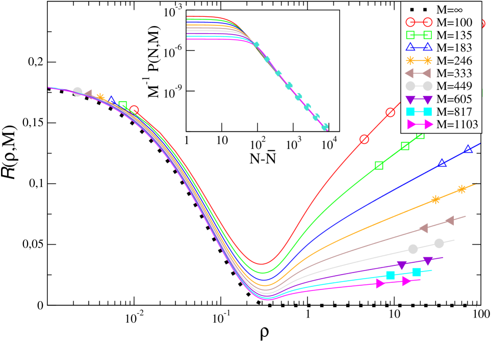
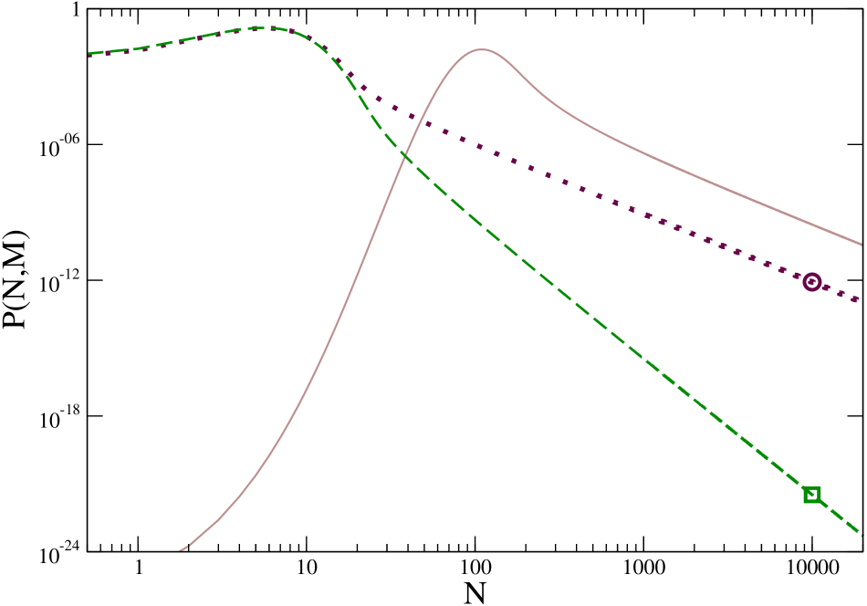
Figure 3: Upper panel: The function ${\cal R}(\rho,M)$ is plotted against $\rho$ for the model with probabilities (6) with a uniform $K_{m}=3>K_{c}$, for the values of $M$ in the key. The heavy-dotted black line is this quantity for $M\to\infty$, which coincide with $R(\rho)$ obtained from Eqs. (8,10) for $\rho\leq\overline{\rho}$ and is identically zero for $\rho\geq\overline{\rho}$. In the inset $M^{-1}P$ is plotted against $N-\overline{N}$. The heavy dotted turquoise line is the law $(N-\overline{N})^{-3}$, i.e. eqs.(16,17). Lower panel: $P$ is plotted for $M=333$ and the three different choices (see text) i) $K_{m}\equiv K=3,\,\forall m$, continuous brown, ii) $K_{m}\equiv K=6,\,\forall m$, green dashed with a square and iii) $K_{1}=3,K_{m}=K=6,\,\forall m>1$, dotted maroon with a circle.

As already discussed, for values of the density larger than $\overline{\rho}$ a straightforward steepest-descent evaluation of the integral in (2) breaks down. In this case $P$ is not exponentially small in $M$, as required by eq. (8), as it can clearly be understood observing in fig. 3 that the dependence on $M$ does not cancels and ${\cal R}$ keeps decreasing to zero for any value of $M$. In this region condensation occurs and, instead of eqs. (8,10), the solution (16,17) applies. In order to see this, in the inset of fig.3 we plot $M^{-1}P(N,M)$, since according to eq. (16,17) this quantity ought to be independent of $M$ and proportional to $p(N-\overline{N})$. As expected, for $\rho\gg\overline{\rho}$ the form (16,17) describes the probability with great accuracy for large $N$. Notice that in the condensed region the convergence to the asymptotic form [eq. (16,17)] is much faster than the one in the gas phase [to eqs. (8,10)], being achieved already for $M\lesssim 100$, a value for which ${\cal R}$ is still quite different from $R$ in the region $\rho<\overline{\rho}$.

V Non identically distributed variables

Now we turn to study the phenomenon of condensation when the microscopic variables are not identically distributed. Specific issues of this and related problems have been addressed in condzrp2 ; condzrp7b ; krug ; bianconi ; igloi1 ; igloi2 ; janowsky ; derrida ; grossinsky . Here we are interest in the derivation of a general form for $P$, generalizing eq. (16), and to discuss the related phenomenon of the giant response on broad grounds.

When the variables are non-identically distributed one can argue that condensation occurs on the most favorable receptor condzrp2 ; condzrp7 , namely the one with the larger $p_{m}(n_{\ell})$. In the example (6), it is the one with the smaller $K_{m}$. Denoting $\overline{m}$ this term [i.e. $p_{\overline{m}}(n_{\ell})>p_{m}(n_{\ell})$ $\forall m\neq\overline{m}$], recalling the physical meaning of $\pi$ in eq. (5), it is clear that a structure like the one in Fig. 3, with a sharp peak around $n_{\ell}$, will be present if the recently added receptor is the one where condensation occurs, namely if $p_{M}\equiv p_{\overline{m}}$ in eq. (5). Then, in order to proceed as in Sec. IV, we define

$$\pi(n,N,M)=P(N-n,M-1)\,p_{\overline{m}}(n),$$ (19)

which amounts only to the choice of a particular labeling of the receptors. Proceeding as in Sec. IV one obtains the following equation

$$C(N,M)=(1-a)P(N,M)\simeq\sigma P(N_{\ell},M-1)p_{\overline{m}}(N-N_{\ell}),$$ (20)

instead of eq. (14), thus arriving at

$$P(N,M)\simeq b_{M}\,p_{\overline{m}}(N-\overline{N})$$ (21)

in place of eq. (16). This form of the probability generalize eqs. (16,17) to the case of non-identically distributed variables. Notice that no assumptions on the form of the microscopic probabilities $p_{m}(n)$ has been made also in this case and, therefore, eq. (21) is expected to hold quite generally. Together with eqs. (16,17), this equation represents the main result of this paper. Notice that the dependence on $M$ of $b_{M}$ can be very different from the one (17) holding for identically distributed variables. Indeed, when the microscopic probabilities depend on $M$, the number of particles in the condensed state may not be simply proportional to $M$, since the $M$-th receptors can promote condensation differently from the previous ones. An example showing this will be shown in Sec. V.2. A straightforward consequence of eq. (21) is the phenomenon of the extreme sensitivity of the global probability $P$ to specific details of the microscopic ones $p_{m}$, that we discuss below.

V.1 Giant response

It must be stressed that the solutions (16,21) are totally different from the one (7), in particular concerning the dependence on $M$. Indeed, while (7) is exponentially small for large $M$ and transforms into a $\delta(N-\overline{N})$, eq. (16,17) shows that in the presence of condensation the dependence can be as weak as linear in $M$, signaling the occurrence of anomalously large fluctuations.

Related to that, an extreme sensitivity of the macroscopic probability $P$ to the details of the microscopic ones $p_{m}$ arises. In fact, eq. (21) clearly shows that the distribution of the single variable $\overline{m}$ fully determines the global quantity $P$. Introducing a susceptibility $\chi$ – the shift of the macroscopic probability due to the variation of a microscopic one – from eq. (21) one has

$$\chi(N,m)=\lim_{M\to\infty}\frac{\Delta P(N,M)}{\Delta p_{m}(N)}=\left\{\begin{array}[]{ll}0\,,&\mbox{gas}\\ B_{M}\,\delta_{m,\overline{m}}\,,&\begin{array}[]{ll}\mbox{condens.}\\ (N\gg\overline{N}),\end{array}\end{array}\right.$$ (22)

where $B_{M}$ is a constant. This shows that in the gas phase a shift of one (or even of a finite number) of the microscopic probabilities cannot alter the global behavior of $P$, since this is determined by the synergic contribution of a number $M\to\infty$ of variables, the situation is profoundly different when condensation occurs. In this case $P$ is fully determined by the statistical properties of the most favorable receptor $\overline{m}$. Therefore $P$ is independent of the form of all the other $M-1$ variables, whereas a macroscopic effect can be determined by altering the statistical properties of the single $p_{\overline{m}}$. As we will show by means of some examples in Sec. V.2 this may have dramatic effects on the form of the probability $P$ in the condensed phase.

This anomalous susceptibility is reminiscent of the large response induced by gapless modes corberi2002 , such as massless Goldstone modes in systems with a spontaneously broken continuous symmetry. Actually, starting from equally distributed variables the symmetry between the receptors is broken by changing the properties of one of them. However the phenomenon of the giant susceptibility discussed here is more general since it occurs also when the modification of the probability of a single variable occurs in a set of (already) non-identically distributed ones, as will be illustrated by the second example of Sec. V.2 (fig. 4). To the best of our knowledge, this remarkable property of the susceptibility (22) was never pointed out before.

V.2 Examples

The occurrence of condensation in the case of non-identically distributed variables and the giant response phenomenon can be illustrated using again the probabilities (6) with $m$-dependent $K_{m}$’s. The simplest non-trivial choice is when all the $K_{m}$’s are equal except one, namely $K_{m}=K$, $\forall m>1$ while $K_{1}$ can be different from $K$.

In the lower panel of fig.3 we compare $P$ for the three cases i) $K_{1}=K=3$, ii) $K_{1}=K=6$ and iii) $K_{1}=3,K=6$. One sees that the curves relative to the choices ii) and iii) coincide for $\rho\leq\overline{\rho}$ (i.e. up to the maximum of $P$). This is because in this region there is no condensation and the macroscopic probability is insensitive to a single $p_{m}$, eq. (22). However, for $\rho>\overline{\rho}$ the two curves become totally different and instead case iii) behaves as i), apart from a vertical displacement due to the different value of the constant $b_{M}$ in eq. (21). This shows that a single variable cannot influence the collective behavior unless it is the one where condensation occurs, in which case a giant response is observed.

The examples considered insofar where based on power-law probabilities (6). However, the features above are more general and not only restricted to this case. We show this by considering the exponential form

$$p_{m}(n)=c\,\exp\left[-K_{m}\cdot n^{\kappa_{m}}\right],$$ (23)

where $K_{m}=\beta\left(\frac{m}{M}\right)^{\alpha}$ ($\beta$ and $c$ are constants), and $\kappa_{m}$ an $M$-independent exponent. This case is interesting also because the microscopic probabilities $p$ do not depend only on $m$, but also on $M$. In this case the scaling (17), which was expected quite generally for $M$-independent $p$’s, can – in principle – be spoiled, and a general form of $b_{M}$ is not available.

In order to illustrate the behavior of $P$ with the exponentially distributed microscopic probabilities we have evaluated it for different choices of the parameters entering eq. (23). Starting with a uniform exponent $\kappa_{m}\equiv\kappa=1$, setting $\beta=1$ and $\alpha=2$, the upper panel of fig.4 shows a pattern of behavior similar to the case (6) with $K>K_{c}$: for $N\leq\overline{N}$, ${\cal R}$ approaches the form (7) with a rate function given by Eqs. (8,9), whereas for $N\gg\overline{N}$ the determination (21) holds (with $\overline{m}=1$), implying $P(N,M)\sim e^{-\frac{(N-\overline{N})}{M^{2}}}$, as shown in the inset. The data collapse is obtained by plotting $M^{2}P(N,M)$ against $(N-\overline{N})/M^{2}$, implying that $b_{M}=bM^{-2}$. Notice that the approach to the asymptotic form is much faster than for the fat-tailed probabilities (6), since already for $M\simeq 100$ one has a good representation of the large-$M$ form in the range of densities considered, at variance with what observed in Fig. 3.

The phenomenon of the giant susceptibility is illustrated by comparing the case above with the one where we change the distribution of $n_{1}$ as to have $\kappa_{1}=0.95$ and all the remaining ones are left untouched ($\kappa_{m}=\kappa,\,\forall\kappa>1$). The lower panel of fig.4 shows that, while in the normal phase $N\leq\overline{N}$ this does not alter $P$ (a residual difference between the two curves is due to the finite value of $M$), a dramatic change is produced in the condensed region $N>\overline{N}$ because, since $\kappa_{1}<\kappa$, the statistical properties of the condensing variable have been changed.

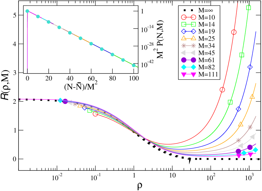
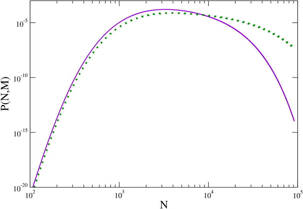
Figure 4: Upper panel: The function ${\cal R}(\rho,M)$ is plotted against $\rho$ for the model with exponential probabilities (see text) with $\beta=1$, $\kappa(m)=\kappa\equiv 1$, $\alpha=2$, for the values of $M$ in the key. The heavy-dotted black line is this quantity for $M\to\infty$, which coincide with $R(\rho)$ obtained from Eqs. (8,9) for $\rho\leq\overline{\rho}$ and is identically zero for $\rho\geq\overline{\rho}$. In the inset $M^{2}P$ is plotted against $(N-\overline{N})/M^{2}$. The heavy dotted turquoise line is the law $e^{-(N-\overline{N})/M^{2}}$, i.e. eq.(21). Lower panel: The $P$ of the main figure with $M=61$ (continuous violet) is compared with the case (dotted green) with $\kappa_{1}=0.95$, $\kappa_{m}\equiv\kappa=1$ $\forall m>1$.

VI Conclusions

In this paper we have discussed the general problem of evaluating the probability distribution $P(N,M)$ of the sum $N$ of a large number $M$ of micro-variables, not necessarily identically distributed.

We have done this by means of the recurrence relation (4), which provides an analogy with a thermodynamic system where a condensation transition occurs and the identification of an order parameter $\rho_{\ell}$. Eq. (4) allows also the derivation of a rather general expression for $P$ [eq. (21)] which is valid, when condensation occurs, for finite values of $M$. From this expression, computing the susceptibility (22), the extreme sensitivity of $P$ to the distribution of even a single variable was explicitly shown.

These properties of the probability $P$ have been discussed by means of specific examples amenable of analytical and numerical computations, including identically and differently distributed variables, with or without fat-tails and also in the case of a specific dependence of the microscopic probabilities $p$ on the number $M$ of micro-variables.

The noteworthy features discussed in this paper are associated to the existence of a condensation phenomenon and, therefore, they are not expected to be only relevant to the large deviations of ${\cal N}$, but also to those of different macrovariables, and to apply to a large class of problems in Physics and other areas, making the issue considered in this paper a broad and general research topic.

VII Appendix: Saddle-point evaluation of $P$ in the condensed phase

In the condensed phase the symmetry between the receptors is broken since, as discussed in Sec. IV, a single variable provides a contribution comparable to all the remaining ones. Let us, without loss of generality, indicate this variable as being the first, namely $n_{1}$. In view of that, we re-write the first line of eq. (2) as follows

$$P(N,M)=\sum_{n_{1}}p(n_{1})\Omega(n_{1},N)$$ (24)

with

$$\Omega(n_{1},N,M)=\sum_{n_{2},n_{3},\dots,n_{M}}p_{2}(n_{2})\cdots p_{M}(n_{M})\,\delta_{{\cal N}_{1},N-n_{1}},$$ (25)

where ${\cal N}_{1}=\sum_{m=2}^{M}n_{m}$. A solution can be found by making the ansatz that in the condensed phase the argument of the sum in eq. (24) is sharply peaked around a certain value $n_{\ell}$, with a certain width $\tilde{b}$, so that it can be evaluated as

$$P(N,M)=M\,\tilde{b}\,p(n_{\ell})\Omega(n_{\ell},N,M)$$ (26)

where $\tilde{b}=\sqrt{2\pi[-(\partial^{2}\ln(p\Omega)/\partial n_{1})_{n_{1}=n_{\ell}}]^{-1}}$ and the factor $M$ in front of the r.h.s. of eq. (26) is due to the $M$ possible ways of choosing the variable denoted by $n_{1}$ among $M$. Using eq. (26) as a starting point, instead of eq. (2), one arrives at

$$P(N,M)=\tilde{b}\,M\,p(n_{\ell})\,\frac{1}{2\pi i}\oint dz\,e^{M[\ln Q(z,M)-(\rho-\rho_{1})\ln z]},$$ (27)

for large $M$, where now

$$Q(z,M)=\left[\prod_{m=2}^{M}\sum_{n_{m}}p_{m}(n_{m})z^{n_{m}}\right]^{\frac{1}{M-1}}$$ (28)

and $\rho_{1}=n_{\ell}/M$ is the condensed particles density. The steepest descend evaluation of the integral leads to the saddle point equation

$$z^{*}(\rho)\,\frac{Q^{\prime}[z^{*}(\rho)]}{Q[z^{*}(\rho)]}=\rho-\rho_{1}.$$ (29)

In the condensed phase there is always a solution with $z=1$ and $\rho_{1}=\rho-\frac{Q^{\prime}(1)}{Q(1)}$, and the evaluation of the integral in eq. (27) gives

$$P(N,M)=b_{M}\,p(n_{\ell})$$ (30)

with $b_{M}\sim\tilde{b}\,M\,e^{M\ln Q(1)}/(2\pi i)=\tilde{b}\,M/(2\pi i)$ (in the last passage we have used $Q(1)\equiv 1$ because of the normalization of the $p$’s). Recalling that $n_{\ell}\simeq N-\overline{N}$ (see Sec. III) one recovers the result (16) that was obtained in a different way – by using the recurrency relation (4) – in Sec. III.

References

- (1) Castellano C., Corberi F. Zannetti M., Phys. Rev. E 56, 4973 (1997).
- (2) Bialas P., Burda Z. Johnston D., Nucl. Phys. B 493, 505 (1997).
- (3) Bialas P., Burda Z. Johnston D., Nucl Phys B 542, 413 (1999).
- (4) Bialas P., Bogacz L., Burda Z. Johnston D., Nucl Phys. B 575, 599 (2000).
- (5) Evans M.R., Braz. J. Phys. 30, 4257 (2000).
- (6) Evans M.R. T.Hanney, J. Phys. A: Math. Gen. 38, R195 (2005).
- (7) Majumdar S.N., Evans M.R. Zia R.K.P., Phys. Rev. Lett. 94, 180601 (2005).
- (8) Godrèche C., Lect. Notes Phys 716, 261 (2007).
- (9) Evans M.R. Waclaw B., J. Phys. A: Math. Theor. 47, 095001 2014.
- (10) L. Ferretti, M. Mamino G. Bianconi, Phys. Rev. E 89, 042810 (2014).
- (11) B. Schmittmann, K. Hwang R. K. P. Zia, Europhys. Lett. 19, 19 (1992).
- (12) M. R. Evans, Europhys. Lett. 36, 13 (1996).
- (13) O.J. O’Loan, M.R. Evans M.E. Cates, Phys. Rev. E 58, 1404 (1998).
- (14) S.N. Majumdar, S. Krishnamurthy M. Barma, Phys. Rev. Lett. 81, 3691 (1998).
- (15) A. Bar D. Mukamel, J. Stat. Mech., P11001 (2014).
- (16) S. Grosskinsky, G. M. Schuetz H. Spohn J. Stat. Phys. 113, 389 (2003).
- (17) Drouffe J-M, Godrèche C Camia F., J. Phys. A: Math. Gen. 31(1), L19 (1998).
- (18) Godrèche C., in Henkel M, Pleimling M, Sanctuary R (Eds.), Ageing and the Glass Transition, Lect. Notes Phys. 716, Springer (2007).
- (19) Godrèche C.Luck JM., J. Phys.: Condens. Matter 14, 1601 (2002).
- (20) Godrèche C. Luck JM., Eur. Phys. J B 23(4), 473 (2001).
- (21) Huang K., Statistical Mechanics John Wiley and Sons eds., New York (1967).
- (22) Zannetti M., Corberi F. Gonnella G., Phys. Rev. E 90, 012143 (2014).
- (23) Zannetti M., Corberi F. Gonnella G., Commun. Theor. Phys. 62, 555 (2014).
- (24) Harris R.J., Rákos A. Schuetz G.M., J. Stat. Mech., P08003 (2005).
- (25) Merhav N. Kafri Y., J. Stat. Mech., P02011 (2010).
- (26) Corberi F. Cugliandolo L.F., J. Stat. Mech., P11019 (2012).
- (27) Corberi F., Gonnella G., Piscitelli A. Zannetti M., J. Phys. A: Math. Theor. 46, 042001 (2013).
- (28) Szavits-Nossan J., Evans M.R. Majumdar S.N., Phys. Rev. Lett. 112, 020602 (2014).
- (29) Szavits-Nossan J., Evans M.R. Majumdar S.N., J. Phys. A: Math. Theor. 47, 042001 (2013).
- (30) Chleboun P. Grosskinsky S., J. Stat. Phys. 140, 846 (2010).
- (31) Gambassi A. Silva A., Phys. Rev. Lett. 109, 250602 (2012).
- (32) Filiasi M., Livan G., Marsili M., Peressi M., Vesselli E. Zarinelli E., J. Stat. Mech.: Theory and Experiment, P09030 (2014).
- (33) Touchette H., Phys. Rep. 478, 1 (2009).
- (34) M.R. Evans S.N. Majumdar, J. Stat. Mech. P05004 (2008).
- (35) M.I. Tribelsky, Phys. Rev. Lett. 89, 070201 (2002).
- (36) J. Krug P.A. Ferrari, J. Phys. A: Mathematical and General 29 (18), L465 (1996).
- (37) G. Bianconi A.-L. Barabási, Phys. Rev. Lett. 86, 5632 (2001).
- (38) R. Juhász, L. Santen F. Iglói. Phys. Rev. E 74, 061101 (2006).
- (39) F. Igloi, R. Juhasz Z. Zimboras, Europhys. Lett. 79, 37001 (2007).
- (40) S.A. Janowsky J.L. Lebowitz, Phys. Rev. A 45, 618 (1992).
- (41) B. Derrida in Statphys19 ed. B-L Hao, (1996) World Scientific.
- (42) S. Grosskinsky, P. Chleboun, G.M. Schütz, Phys. Rev. E 78, 030101(R) (2008).
- (43) F. Corberi, E. Lippiello M. Zannetti, Phys. Rev. E 65, 046136 (2002). R. Burioni, F. Corberi A. Vezzani, J. Stat. Mech. (2009) P02040.