Wave propagation on Euclidean surfaces with conical singularities. I: Geometric diffraction.

Abstract.

We investigate the singularities of the trace of the half-wave group, $\operatorname{Tr}e^{-it\sqrt{\Delta}}$, on Euclidean surfaces with conical singularities $(X,g)$. We compute the leading-order singularity associated to periodic orbits with successive degenerate diffractions. This result extends the previous work of the third author [Hil] and the two-dimensional case of the work of the first author and Wunsch [ForWun] as well as the seminal result of Duistermaat and Guillemin [DuiGui] in the smooth setting. As an intermediate step, we identify the wave propagators on $X$ as singular Fourier integral operators associated to intersecting Lagrangian submanifolds, originally developed by Melrose and Uhlmann [MelUhl].

0. Introduction

In this article, we investigate the spectral geometry of Euclidean surfaces with conical singularities $(X,g)$. We determine the precise microlocal structure of the half-wave propagator, $e^{-it\sqrt{\Delta}}$, near a ray that undergoes one or two degenerate diffractions. Using this, we compute the leading-order singularity of the trace of the half-wave group, $\operatorname{Tr}e^{-it\sqrt{\Delta}}$, associated to an isolated periodic orbit undergoing two degenerate diffractions through cone points. For example, if the periodic orbit has length $L$ and undergoes degenerate diffractions through two cone points at a distance $b$ apart, we show that the associated wave trace singularity is

(0.1) $$\frac{1}{4i\pi^{2}}\cdot\sqrt{b(L-b)}\cdot(t-L-i0)^{-1}.$$

0.1. Background

Spectral geometry typically aims at understanding the relations between the spectrum of the Laplace operator on a Riemannian manifold and the geometry of the associated geodesic flow. These relations may be revealed by the study of wave propagation. For instance, the Poisson relation states that the trace of the wave propagator is smooth except possibly at the lengths of periodic orbits. Moreover, in a generic and smooth situation, the singularity that is brought to the wave trace by a particular periodic orbit can be fully understood and leads to the definition of the so-called wave-invariants (see [DuiGui]). These wave-invariants may then be used for instance in inverse spectral problems. They also serve as a particular motivation to study wave propagation on different kind of singular surfaces. We will focus on Euclidean surfaces with conical singularities since this general setting includes polygonal billiards and translation surfaces, both of which are very interesting and natural.

The basic new feature of wave propagation on singular manifolds is the dichotomy between waves that hit the singularity—that are then diffracted in all possible directions—and waves that miss the singularity and propagate according to the usual laws for smooth manifolds. This fact leads to the definition of the so-called geometric (or direct) front that consists of rays that miss the vertex and the diffracted front that consists of rays that hit the vertex and are reemitted in all possible directions. On a two dimensional cone, these two fronts share two rays in common that correspond to the limit of rays that nearly miss the cone point from one side or the other. In the literature, these two rays are called either “geometrically diffractive” [MelWun] or “singular diffractive” [Hil]. We will use here the former terminology. On a compact surface with conical singularities the situation becomes quickly complicated for a diffractive ray may hit successive conical points and experience new diffractions that may be singular and so on. These diffractive phenomena are established in the quite abundant literature on wave propagation on singular manifolds starting with Sommerfeld’s result for Euclidean sectors or cones [Som]. Among the important milestones of this story are the studies by Cheeger and Taylor for cones of exact product-type [CheTay1, CheTay2] and by Melrose and Wunsch in the general case [MelWun].

Over the years, there has been investigation of the impact of diffraction on the wave-trace. For instance, Wunsch showed in [Wun] that singularities may appear at length of periodic diffractive orbits. For some periodic diffractive geodesics, the leading singularity is then computed in [Hil] in the Euclidean case and in [ForWun] in a more general case (see also [BogoPavSch] for related results from a physics perspective). Both these results are built upon a precise description of the wave propagator that is microlocalized in the vicinity of given periodic (possibly diffractive) geodesic. However, none of these studies attempted to determine the precise microlocal nature of the propagator near a geometrically diffractive ray: in [ForWun], it is assumed that no geometric diffraction occurs (with a non-focusing assumption that would be automatically satisfied in our case), while in [Hil], it is assumed that the periodic geodesic has at most one geometric diffraction. The main purpose of the present paper is to fill this gap, i.e., to give a precise microlocal description of the wave propagator near the geometric diffractive rays, on an ESCS. More precisely, we will identify the microlocalized propagator near a ray that undergoes one or two geometric diffractions as an element of the Melrose-Uhlmann class of singular Fourier Integral Operators ([MelUhl]), associated to either two, or four, Lagrangian submanifolds. One advantage of this identification is the ease of computing wave trace singularities, such as (0.1), using standard methods such as stationary phase.

This is the first article in a planned series of three. In the second paper, we will show how to compute wave traces for any closed orbit on an ESCS (with any number of geometric diffractions). In the third paper, we will apply our results to inverse spectral results, specifically isospectral compactness in the class of ESCSs. To keep the length of the present paper within reasonable bounds, we restrict our attention here to at most two geometric diffractions.

0.2. Cones and ESCSs

The Euclidean cone of cone angle $\alpha>0$ is the product manifold $C_{\alpha}\stackrel{{\scriptstyle\textup{def}}}{{=}}\left(\mathbb{R}_{+}\right)_{r}\times\left(\mathbb{R}/\alpha\mathbb{Z}\right)_{\theta}$ equipped with the exact warped product metric

$$ds^{2}\stackrel{{\scriptstyle\textup{def}}}{{=}}dr^{2}+r^{2}\,d\theta^{2}.$$

The vertex of the cone $\bm{p}$ is the point where all $(0,\theta)$ are identified, and we will denote by $C_{\alpha}^{\circ}\stackrel{{\scriptstyle\textup{def}}}{{=}}C_{\alpha}\setminus\{\bm{p}\}$ the cone without its vertex. Let us recall that the Euclidean distance on $C_{\alpha}$ between two points $\bm{q}_{1}=(r_{1},\theta_{1})$ and $\bm{q}_{2}=(r_{2},\theta_{2})$ in polar coordinates is:

(0.2) $$\begin{cases}\mbox{dist}(\bm{p},\bm{q}_{1})=r_{1},&\\ \mbox{dist}(\bm{q}_{1},\bm{q}_{2})=r_{1}+r_{2},&|\theta_{2}-\theta_{2}|>\pi\\ \mbox{dist}(\bm{q}_{1},\bm{q}_{2})=\sqrt{r_{1}^{2}+r_{2}^{2}-2r_{1}r_{2}\cos(\theta_{2}-\theta_{1})},&|\theta_{2}-\theta_{1}|\leqslant\pi.\\ \end{cases}$$

A Euclidean surface $X$ with conical singularities (denoted by ESCS in the sequel) is a singular Riemannian surface such that any point has a neighbourhood that is isometric either to a Euclidean ball in $\mathbb{R}^{2}$ or to a ball centered at the vertex of some Euclidean cone $C_{\alpha}$.

Example 0.1.

From any polygonal domain $\Omega$ in the plane we may generate an ESCS by taking two copies of the polygon, reflecting one of these copies across the $y$-axis, and identifying the corresponding sides. Starting from a square, we build in this way a surface that is topologically a sphere that is flat with four singularities of angle $\pi.$

Example 0.2.

More generally, a surface that is obtained by gluing Euclidean polygons along their sides also is Euclidean with conical singularities. The surface of a cube is a ESCS that is topologically a sphere with $8$ singularities of angle $\frac{3\pi}{2}.$

Let $X$ be a Euclidean surface with conical singularities, and let $\mathbf{P}$ be the set of its conical points. Define $X^{\circ}\stackrel{{\scriptstyle\textup{def}}}{{=}}X\setminus\mathbf{P}$. Let $u$ be a smooth function that vanishes near the conical points. Using the Euclidean metric, one defines the gradient of $u$, $\nabla u$, and the action of the Laplacian on $u$, $\Delta u$, as usual. The Laplace operator thus defined is not essentially self-adjoint. Among the possible self-adjoint extensions, the most natural one is the Friedrichs extension that is associated with the Dirichlet energy quadratic form

$$Q(u)\stackrel{{\scriptstyle\textup{def}}}{{=}}\int_{X}\left|\nabla u\right|^{2}dS,\quad u\in C_{c}^{\infty}(X^{\circ}),$$

where $dS$ is the Euclidean area measure. Throughout the paper $\Delta$ will always define the Friedrichs extension of the Euclidean Laplace operator. By choice it is a non-negative operator.

Writing $\text{\qed}=D_{t}^{2}-\Delta$ with $D_{t}=\frac{1}{i}\,\partial_{t},$ the associated wave operator is then defined as

(0.3) $$\left\{\begin{aligned} &\text{\qed}_{g}u(t,x)=0\\ &u(0,x)=u_{0}(x)\\ &\partial_{t}u(0,x)=\dot{u}_{0}(x)\end{aligned}\right.$$

We will always take $t\geqslant 0$. The wave propagators that are associated with this wave equation may be defined through functional calculus and we denote them by:

(0.4) $$\mathbf{W}(t)\stackrel{{\scriptstyle\textup{def}}}{{=}}\frac{\sin\!\left(t\sqrt{\smash[b]{\Delta}}\right)}{\sqrt{\smash[b]{\Delta}}}\qquad\text{and}\qquad\dot{\mathbf{W}}(t)\stackrel{{\scriptstyle\textup{def}}}{{=}}\cos\!\left(t\sqrt{\smash[b]{\Delta}}\right).$$

We will also use the half-wave propagator $\mathcal{U}(t)\stackrel{{\scriptstyle\textup{def}}}{{=}}\exp(-it\sqrt{\Delta}).$

Since singularities of solutions to the wave equation propagate with finite speed, the propagator $\mathbf{W}(t)$ can be understood by patching together local propagators that are defined either on the plane or on $C_{\alpha}.$ As a first step it is therefore crucial to understand wave propagation on the flat cone $C_{\alpha}$.

0.3. The wave kernel on cones

It turns out that the wave kernel on $C_{\alpha}$ is explicitly known (see [Som, CheTay1, CheTay2, Fri] for different ways of constructing this kernel — we describe these briefly at the beginning of Sections 2 and 3). Propagation of singularities for the wave equation on $C_{\alpha}$ is then described as follows. Using polar coordinates, we define on $(0,\infty)\times T^{*}C_{\alpha}^{\circ}\times T^{*}C_{\alpha}^{\circ}$ two Lagrangian submanifolds $\Lambda^{\bm{\mathsf{G}}}$ and $\Lambda^{\bm{\mathsf{D}}}$. For $\alpha>\pi$, these can be defined as follows.

The geometric (or “main”) Lagrangian is

(0.5a) $$\Lambda^{\bm{\mathsf{G}}}\stackrel{{\scriptstyle\textup{def}}}{{=}}N^{*}\!\left\{t^{2}=r_{1}^{2}+r_{2}^{2}-2r_{1}r_{2}\cos(\theta_{1}-\theta_{2})\text{ and }|\theta_{1}-\theta_{2}|\leqslant\pi\right\},$$

the diffractive Lagrangian is

(0.5b) $$\Lambda^{\bm{\mathsf{D}}}\stackrel{{\scriptstyle\textup{def}}}{{=}}N^{*}\!\left\{t^{2}=\left(r_{1}+r_{2}\right)^{2}\right\},$$

and their intersection is the singular set

(0.5c) $$\Sigma\stackrel{{\scriptstyle\textup{def}}}{{=}}\Lambda^{\bm{\mathsf{G}}}\cap\Lambda^{\bm{\mathsf{D}}}=\Lambda^{\bm{\mathsf{D}}}\cap\{|\theta_{1}-\theta_{2}|=\pi\}.$$

In the case $\alpha\leq\pi$, we choose an integer $N$ such that $\alpha N>\pi$. Then we consider the $N$-fold covering map from $C^{\circ}_{N\alpha}$ to $C^{\circ}_{\alpha}$ induced by the natural map $\mathbb{R}/N\alpha\mathbb{Z}\to\mathbb{R}/\alpha\mathbb{Z}$. As this is a local isometry, this induces a covering map $T^{*}C^{\circ}_{N\alpha}\to T^{*}C^{\circ}_{\alpha}$. We define $\Lambda^{\bm{\mathsf{G}}}_{\alpha}$ to be the image of $\Lambda^{\bm{\mathsf{G}}}_{N\alpha}$ under this covering map.

The terminology indicates that $\Lambda^{\bm{\mathsf{G}}}$ corresponds to geometric, or non-diffractive geodesics (i.e., geodesics on $C_{\alpha}$ that avoid $\bm{p}$) which carry the main singularity whereas $\Lambda^{\bm{\mathsf{D}}}$ corresponds to diffractive geodesics (i.e., concatenation of two rays emanating from $\bm{p}$.) The singular set thus corresponds to diffractive geodesics that are limits of non-diffractive ones. We will refer to these as geometrically diffractive. We will denote by $\Lambda^{{\bm{\mathsf{G}}}/{\bm{\mathsf{D}}}}_{\pm}$ the Lagrangian submanifolds obtained by restricting $\Lambda^{{\bm{\mathsf{G}}}/{\bm{\mathsf{D}}}}$ to $\mp\tau>0$ where $\tau$ is the dual variable to $t.$

The explicit expression of the propagator implies, first, that singularities propagate according to $\Lambda^{\bm{\mathsf{G}}}\cup\Lambda^{\bm{\mathsf{D}}}$, and second, that away from the intersection $\Sigma$ the propagator is a classical Fourier Integral Operator (FIO). Away from the intersection $\Sigma$, the kernel of the half-wave propagator $e^{-it\sqrt{\Delta}}$ is given by the so-called Geometric Theory of Diffraction (see Appendix B).

0.4. Main results

Our first result is a precise description of the kernel of the wave propagator on the cone $C_{\alpha}$ near the singular set $\Sigma.$ It is actually a bit simpler to describe the result for the half-wave propagator $e^{-it\sqrt{\Delta}}$, whose Schwartz kernel we denote by $\bm{U}_{\alpha}.$

We observe that $(t^{*},\bm{q}_{1}^{*},\bm{q}_{2}^{*})$ is in the projection of $\Sigma$ on $(0,\infty)\times C_{\alpha}^{\circ}\times C_{\alpha}^{\circ}$ if and only if, in polar coordinates, we have $r_{1}^{*}+r_{2}^{*}=t^{*}$ and $\theta_{1}^{*}-\theta_{2}^{*}=\epsilon\pi,\,\epsilon=\pm 1.$ Let $\gamma$ be the parametrization by arclength of the geometrically diffractive geodesic that joins $\bm{q}_{1}^{*}$ to $\bm{q}_{2}^{*}$ normalized in such a way that $\gamma(-r_{2}^{*})=\bm{q}_{2},~{}\gamma(0)=\bm{p},~{}\gamma(r_{1}^{*})=\bm{q}_{1}.$ Since the cone is flat, $\gamma$ can be extended to a local isometry $\mathcal{I}_{\epsilon}$ that is defined on $\mathbb{R}^{2}\setminus\{(0,\epsilon y),~{}y>0,\,\epsilon=\pm 1\,\}.$ Using $\mathcal{I}_{\epsilon}$ we can thus parametrize a neighbourhood of $(\bm{q}_{1}^{*},\bm{q}_{2}^{*})$ in $C_{\alpha}^{\circ}\times C_{\alpha}^{\circ}$ by the product of two Euclidean balls in $\mathbb{R}^{2}$ the first one centered at $(r_{1}^{*},0)$ and the second one at $(-r_{2}^{*},0)$ (in Euclidean coordinates).

Theorem 0.3.

Let $\bm{q}_{1}^{*}$ and $\bm{q}_{2}^{*}$ be the extremities of a geometrically diffractive geodesic of length $t^{*}$ and diffraction angle $\epsilon\pi$ ($\epsilon=\pm 1).$ Locally near $(t^{*},\bm{q}_{1}^{*},\bm{q}_{2}^{*})$ in $(0,\infty)\times C_{\alpha}^{\circ}\times C_{\alpha}^{\circ}$ the kernel $\bm{U}_{\alpha}$ can be written as the following oscillatory integral:

(0.6) $$\bm{U}_{\alpha}(t,\bm{q}_{1},\bm{q}_{2})=(2\pi)^{-2}\int_{s\geq 0}\int_{\omega>0}e^{i\phi_{\epsilon}(t,\bm{q}_{1},\bm{q}_{2},s,\omega)}a_{\alpha,\epsilon}(t,\bm{q}_{1},\bm{q}_{2},s,\omega)\,d\omega ds$$

where (using $\mathcal{I}_{\epsilon}$ for parametrization—i.e., $g_{\epsilon}(x_{1},y_{1})=\bm{q}_{1},~{}g_{\epsilon}(x_{2},y_{2})=\bm{q}_{2}$)

1. the phase $\phi_{\epsilon}$ is defined by

   $$\phi_{\epsilon}(t,\bm{q}_{1},\bm{q}_{2},s,\omega)=\omega\left[\sqrt{x_{1}^{2}+(y_{1}+s\epsilon)^{2}}+\sqrt{{x_{2}}^{2}+({y_{2}}+s\epsilon)^{2}}-t\right],$$

2. the amplitude $a_{\alpha,\epsilon}$ is a classical symbol that is smooth in $(t,\bm{q}_{1},\bm{q}_{2},s)$ and of order $1$ in $\omega$ so that we have

   $$a_{\alpha,\epsilon}\sim\sum_{k\geq 0}a_{\alpha,\epsilon,1-k}(t,\bm{q}_{1},\bm{q}_{2},s)\,\omega^{1-k}.$$

3. In polar coordinates, we have at leading order

   $$a_{\alpha,\epsilon}(\bm{q}_{1},\,\bm{q}_{2}\,,\,s=0,\omega)=-2\pi i\epsilon\cdot\frac{S_{\alpha}(\theta_{1}-\theta_{2})}{(r_{1}r_{2})^{\frac{1}{2}}}\cdot\Big{[}\sin\theta_{1}+\sin\theta_{2}\Big{]}\cdot\omega.$$

   where $S_{\alpha}$ is the (absolute) scattering matrix for the cone $C_{\alpha}$. An explicit expression for $S_{\alpha}$ is given by (B.11).

From this expression we deduce the following corollary.

Theorem 0.4.

The half-wave propagator $\mathcal{U}_{\alpha}(t)$ on the Euclidean cone $C_{\alpha}$ is in the Melrose-Uhlmann class $I^{m}(\Lambda^{\bm{\mathsf{D}}}_{+},\Lambda^{\bm{\mathsf{G}}}_{+})$ of singular Fourier Integral operators. The order $m$ is equal to $0$ if $t$ is regarded as a parameter, or $-1/4$ if $t$ is regarded as a ‘spatial’ variable. Similarly, the sine propagator $\mathbf{W}(t)$ on the Euclidean cone $C_{\alpha}$ is in the Melrose-Uhlmann class $I^{m-1}(\Lambda^{\bm{\mathsf{D}}},\Lambda^{\bm{\mathsf{G}}})$ of singular Fourier Integral operators.

It can be noted that elements of this class are standard FIOs away from the intersection $\Sigma$ so that this theorem doesn’t say anything new away from $\Sigma$. On the other hand, although the explicit expression of the propagator was already known near $\Sigma$, the fact that it belonged to the Melrose-Uhlmann class was not. It is also worth remarking that it may be possible to obtain the latter theorem by some brute computations starting from the explicit expression of the propagator. We propose a different method, the ‘moving conical point’ method, that exploits geometric features of wave propagation on cones. It has the advantage that the parameter $s$ in (0.6) then has geometric significance: it is the distance by which the conical point is shifted.

Remark 0.5.

It is actually convenient to use the Riemannian metric to identify functions and half-densities. This amounts to multiply the oscillatory integral representation by the half-density $|d\bm{q}^{\prime}d\bm{q}|^{\frac{1}{2}}$ or $|dtd\bm{q}^{\prime}d\bm{q}|^{\frac{1}{2}}$.

Remark 0.6.

Recall (or see Section 1) that in the Melrose-Uhlmann calculus, the order of the distribution on the first Lagrangian $\Lambda^{\bm{\mathsf{D}}}$ is $\frac{1}{2}$-order less than on the second, $\Lambda^{\bm{\mathsf{G}}}$. This allows to recover the fact that the diffracted wave is $\frac{1}{2}$-order smoother (in a Sobolev sense) than the direct wave (in two dimensions).

The oscillatory integral representation of the preceding theorem has several interesting applications mainly because it allows one to compute simply the wave propagator on an ESCS when microlocalized near a geodesic with several geometric diffractions. We will illustrate this by obtaining, for a geodesic with two geometric diffractions in a row an oscillatory integral representation that fits into the class of singular FIO that is constructed in [MelUhl, Sections 7–10] and associated with a system of four intersecting Lagrangians. More precisely, consider a geodesic of length $t$ between $\bm{q}$ and $\bm{q}^{\prime}$ with two geometric diffractions at $\bm{p}_{1}$ and $\bm{p}_{2}$. There are four types of nearby geodesics:

1. non-diffractive geodesics;

2. geodesics that are diffractive at $\bm{p}_{1}$ but not at $\bm{p}_{2}$;

3. non-diffractive geodesics at $\bm{p}_{1}$ that diffract at $\bm{p}_{2}$; and

4. geodesics that diffracts at $\bm{p}_{1}$ and $\bm{p}_{2}.$

Each type corresponds to a particular Lagrangian and these four Lagrangians form a intersecting system in the sense of [MelUhl].

Using the preceding theorem and standard stationary phase arguments we obtain the theorem.

Theorem 0.7.

Microlocally near a geodesic with two geometric diffractions, the half-wave propagator on a ESCS is in the Melrose-Uhlmann class of operators associated with a system of four intersecting Lagrangians.

We actually get much more accurate information since we can derive the principal symbol of the half-wave propagator on the twice diffracted front — see (4.15) and (4.16).

Finally we will use our new expression for $\bm{U}_{\alpha}$ to compute the contribution to the wave-trace of an isolated periodic geodesic with two geometric diffractions.

Proposition 0.8.

On a ESCS, the leading contribution to the wave trace of an isolated periodic diffractive orbit with two geometric diffractions is

$$-\frac{1}{4i\pi^{2}}\cdot\sqrt{b(L-b)}\cdot(t-L-i0)^{-1}.$$

This is perhaps the simplest setting for which neither [ForWun] nor [Hil] applies. This proposition shows that such a geodesic creates in the wave-trace a singularity that is comparable to the singularity that is created in a smooth setting by an isolated periodic orbit. The singularity is $\frac{1}{2}$ stronger than a diffractive geodesic with one non-geometric diffraction and $\frac{1}{2}$ weaker than a cylinder of periodic orbits.

With our new representation of the wave kernel, it should actually be possible to compute the full asymptotic expansion of the contribution to the wave-trace of any kind of periodic diffractive geodesic. This is a far-reaching generalization of results in [Hil] and it leads to the possible computation of many wave-invariants. This opens new questions concerning inverse spectral problems in this kind of geometric setting which, we recall, includes Euclidean polygons. For instance it can be asked whether the full asymptotic expansion of a particular geodesic allows to recover the full picture describing the geodesic: that is the number of diffractions, the lengths of the legs between two diffractions, the diffraction angles and the angles of the cone at which the diffractions occur. We will tackle some of these questions in the second and third parts of this series.

0.5. Organisation of the paper

In Section 1 we will recall the definition of singular Fourier Integral Operators as defined in [MelUhl]. We will first study the case of two intersecting Lagrangians. We will give the oscillatory integral representation using a phase function that depends on an extra parameter $s$. We will then give the generalization to a system of four intersecting Lagrangians.

In Section 2 we will study wave propagation on a cone of total angle $4\pi.$ The first reason why we study this particular cone is that it is the simplest case in which we can implement our method of ‘moving the conical point’ that leads to our new expression for the wave propagator. The fact that the wave propagator belongs to the Melrose-Uhlmann class can then be directly read off from this expression. It is also worth remarking that, in this case the extra parameter $s$ has a geometric meaning since it represents the amount of which the conical point has moved.

The second reason why we can first study the cone of angle $4\pi$ is that the most singular part of the wave propagator near $\Sigma$ actually does not depend on its angle. This can be seen using the construction of the wave kernel made by Friedlander in [Fri]. We will recall this fact in Section 3 and then proceed to prove Theorem 0.3.

In Section 4 we will use Theorem 0.3 to compute the wave propagator when microlocalized near some particular kind of geodesics. We will focus on the case of a geodesic with two geometric diffractions for which a desciption of the microlocalized propagator is not already available in the literature.

In Section 5 we will end this paper by computing the leading contribution to the wave-trace of an isolated periodic orbit with two geometric diffractions.

1. Intersecting Lagrangian distributions

The class of distributions central to our study of the wave propagators on $C_{\alpha}$ is that of intersecting Lagrangian distributions, introduced by Melrose and Uhlmann [MelUhl]. These are distributions whose singularities (in terms of wavefront set) lie along a pair of conic Lagrangian submanifolds $(\Lambda_{0},\Lambda_{1})$ of the cotangent bundle. Here, $\Lambda_{1}$ is a manifold with boundary, and $\Lambda_{0}$ and $\Lambda_{1}$ intersect cleanly at $\partial\Lambda_{1}$. In particular, the intersection is codimension $1$ in both Lagrangians. These distributions were introduced to construct fundamental solutions to operators of real principal type. An analogous class of distributions associated to four intersecting Lagrangian submanifolds, also introduced in [MelUhl], will show up in our study of the wave kernel on a ESCS after two diffractions—see Section 1.3.

1.1. Model Lagrangian submanifolds

Let $X$ be a manifold, and let $(\Lambda_{0},\Lambda_{1})$ be a pair of conic Lagrangian submanifolds of $T^{*}X\setminus\{0\}$ with the geometry described above: $\Lambda_{1}$ is a manifold with boundary, and $\Lambda_{0}$ and $\Lambda_{1}$ intersect cleanly at $\partial\Lambda_{1}$. Moreover, let $q\in\Lambda_{0}\cap\Lambda_{1}$ be a point in the intersection. Melrose and Uhlmann showed that there is a normal form for this geometry. Indeed, let $(\tilde{\Lambda}_{0},\tilde{\Lambda}_{1})$ be the model Lagrangian submanifolds in $T^{*}\mathbb{R}^{n}$:

(1.1) $$\Lambda_{0} =N^{*}\{0\}=\{(x,\xi):x=0,\}$$

$$\Lambda_{1} =N^{*}\{x^{\prime}=0,x_{1}\geq 0\}=\{(x,\xi):x^{\prime}=0,\xi_{1}=0,x_{1}\geq 0\}.$$

Here we decompose $x=(x_{1},x^{\prime})$, where $x^{\prime}=(x_{2},\dots,x_{n})$; similarly, $\xi=(\xi_{1},\xi^{\prime})$. Choose any point $\tilde{q}\in\tilde{\Lambda}_{0}\cap\tilde{\Lambda}_{1}$. Then Melrose and Uhlmann showed that there is a homogeneous sympectic map from a conic neighbourhood of $\tilde{q}$ to a conic neighbourhood of $q$, such that $\tilde{\Lambda}_{i}$ gets mapped to $\Lambda_{i}$. To define intersecting Lagrangian distributions, they first defined them in the model situation. We recall this definition.

Definition 1.1 (Melrose-Uhlmann).

An intersecting Lagrangian distribution of order $m$ associated to the model pair $(\tilde{\Lambda}_{0},\tilde{\Lambda}_{1})$ is a distributional half-density given by an oscillatory integral of the form

(1.2) $$(2\pi)^{-n-\frac{1}{2}}\int\int_{0}^{\infty}e^{i(x\cdot\xi-s\xi_{1})}a(x,s,\xi)\,ds\,d\xi|dx|^{\frac{1}{2}}$$

where $a$ is smooth, compactly supported in $x$ and $s$, and a symbol of order $m+\frac{1}{2}-\frac{n}{4}$ in $\xi$. The space of such distributions is denoted $I^{m}(X;\tilde{\Lambda}_{0},\tilde{\Lambda}_{1})$.

It is shown in [MelUhl] that elements of $I^{m}(X;\tilde{\Lambda}_{0},\tilde{\Lambda}_{1})$ are Lagrangian distributions of order $m$ on $\tilde{\Lambda}_{1}$ when microlocalized away from $\tilde{\Lambda}_{0}$, and Lagrangian distributions of order $m-\frac{1}{2}$ on $\tilde{\Lambda}_{0}$ when microlocalized away from $\tilde{\Lambda}_{1}$. Also, they showed that the space $I^{m}(X;\tilde{\Lambda}_{0},\tilde{\Lambda}_{1})$ is invariant under the action of Fourier integral operators that fix $\tilde{\Lambda}_{0}$ and $\tilde{\Lambda}_{1}$. Consequently, one can define intersecting Lagrangian distributions for a general pair $(\Lambda_{0},\Lambda_{1})$ to be the image of the model space $I^{m}(X;\tilde{\Lambda}_{0},\tilde{\Lambda}_{1})$ under an FIO mapping $\tilde{\Lambda}_{i}$ to $\Lambda_{i}$. The precise definition is as follows:

Definition 1.2.

Let $(\Lambda_{0},\Lambda_{1})$ be a pair of intersecting conic Lagrangian distributions in $T^{*}X\setminus\{0\}$ with the geometry described above. The space $I^{m}(X;\Lambda_{0},\Lambda_{1})$ consists of those distributional half-densities $u$ that can be written as a locally finite sum

$$u=u_{0}+u_{1}+\sum_{i}F_{i}(v_{i})+u_{\infty},$$

where $u_{0}\in I^{m-\frac{1}{2}}(X;\Lambda_{0})$, $u_{1}\in I^{m}(X;\Lambda_{1}\setminus\Lambda_{0})$, $v_{i}\in I^{m}(X;\tilde{\Lambda}_{0},\tilde{\Lambda}_{1})$, $F_{i}$ are FIOs mapping $(\tilde{\Lambda}_{0},\tilde{\Lambda}_{1})$ to $(\Lambda_{0},\Lambda_{1})$, and $u_{\infty}$ is $\mathcal{C}^{\infty}$.

In what follows, we will often omit the space ‘$X$’ from the notation for these distributions, i.e., we will write $I^{m}(\Lambda_{0},\Lambda_{1})$ in the place of $I^{m}(X;\Lambda_{0},\Lambda_{1})$.

1.2. Parametrization of intersecting Lagrangian submanifolds

Over the course of this paper, we will construct the fundamental solution of the wave kernel on a two-dimensional cone directly; we will want to be able to identify it as an intersecting Lagrangian distribution. To do this, we need a direct definition of intersecting Lagrangian distribution in terms of a phase function parametrizing a given pair $(\Lambda_{0},\Lambda_{1})$ in place of the indirect Definition 1.2.

Definition 1.3.

Let $(\Lambda_{0},\Lambda_{1})$ be a pair of intersecting Lagrangian submanifolds, and let $q\in\Lambda_{0}\cap\Lambda_{1}$ be a point in the intersection. A local parametrization of $(\Lambda_{0},\Lambda_{1})$ near $q$ is a function $\phi(x,\theta,s)$, defined in neighbourhood of $(x_{0},\theta_{0},0)\subseteq X\times\mathbb{R}^{k}\times\mathbb{R}_{\geqslant 0}$ such that

• $d_{\theta,s}\phi(x_{0},\theta_{0},0)=0$, and $q=(x_{0},d_{x}\phi(x_{0},\theta_{0},0))$;

• the differentials

  $$d_{x,\theta}\bigg{(}\frac{\partial\phi}{\partial\theta_{i}}\bigg{)}\quad\text{and}\quad d_{x,\theta}\bigg{(}\frac{\partial\phi}{\partial s}\bigg{)}$$

  in the $(x,\theta)$ directions are linearly independent at $(x_{0},\theta_{0},0)$;

• the map

  (1.3) $$C_{0}\stackrel{{\scriptstyle\textup{def}}}{{=}}\{(x,\theta):d_{\theta}\phi(x,\theta,0)=0\}\mapsto\{(x,d_{x}\phi(x,\theta,0))\}\subseteq T^{*}X$$

  is a local diffeomorphism from $C_{0}$ onto a neighbourhood of $q$ in $\Lambda_{0}$;

• the map

  (1.4) $$C_{1}\stackrel{{\scriptstyle\textup{def}}}{{=}}\{(x,\theta,s):d_{\theta,s}\phi(x,\theta,s)=0,\ s\geq 0\}\mapsto\{(x,d_{x}\phi(x,\theta,s))\}\subseteq T^{*}X$$

  is a local diffeomorphism from $C_{1}$ onto a neighbourhood of $q$ in $\Lambda_{1}$.

Let us make some remarks about the definition above. The second condition ensures that the sets $C_{0}$ is a smooth submanifold of $X\times\mathbb{R}^{k}$ of dimension $n=\dim X$, and $C_{1}$ is a smooth submanifold of $X\times\mathbb{R}^{k}\times\mathbb{R}_{\geqslant 0}$ of dimension $n$ transverse to $\{s=0\}$. This makes it possible to speak of diffeomorphisms from $C_{i}$ to $\Lambda_{i}$ as in the third and fourth conditions. The first condition simply says that the base point $(x_{0},\theta_{0},0)$ corresponds to the base point $q$.

Proposition 1.4.

(i) Let $(\Lambda_{0},\Lambda_{1})\subseteq T^{*}X$ be a pair of intersecting Lagrangian submanifolds, and let $q$ be a point in the intersection. Then there exists a local parametrization of $(\Lambda_{0},\Lambda_{1})$ near $q$.

(ii) Let $\phi$, defined in a neighbourhood $U$ of $(x_{0},\theta_{0},0)\in X\times\mathbb{R}^{k}\times R_{\geq 0}$, be a local parametrization of $(\Lambda_{0},\Lambda_{1})$ near $q$. Let $a(x,\theta,s)$ be a classical symbol of order $m-\frac{k}{2}+\frac{1}{2}+\frac{n}{4}$ in the $\theta$ variables which is compactly supported in $U$. Then the oscillatory integral

(1.5) $$(2\pi)^{-\frac{k}{2}-\frac{n}{4}-\frac{1}{2}}\int_{\mathbb{R}^{k}}\int_{0}^{\infty}e^{i\phi(x,\theta,s)}a(x,\theta,s)\,ds\,d\theta\,|dx|^{\frac{1}{2}}$$

is in $I^{m}(\Lambda_{0},\Lambda_{1})$.

Proof.

(i) By [MelUhl], there is a homogeneous canonical transformation $\chi$ defined in a neighbourhood of $\tilde{q}\in\tilde{\Lambda}_{0}\cap\tilde{\Lambda}_{1}$ mapping $\tilde{\Lambda}_{0}$ to $\Lambda_{0}$ and $\tilde{\Lambda}_{1}$ to $\Lambda_{1}$, and sending $\tilde{q}$ to $q$. Let $\Psi(x,y,\theta)$ be a phase function parametrizing the graph of this canonical transformation. Consider the sum of the phase functions

$$\Psi(x,y,\theta)+y\cdot\eta-\eta_{1}s,$$

where the second phase function is the standard parametrization of the model Lagrangian pair. Following [HorFIO]*p. 175, we define a new variable

$$Y=|\theta|y.$$

We then write this sum of the phase functions in terms of $Y$. That is, we define

$$\phi(x,Y,\theta,\eta,s)=\Psi\!\left(x,\frac{Y}{|\theta|},\theta\right)+\frac{Y}{|\theta|}\cdot\eta-\eta_{1}s.$$

Notice that $\phi$ is homogeneous of degree 1 in the variables $(Y,\theta,\eta)$. We claim that $\phi$ is a nondegenerate local parametrization of $(\Lambda_{0},\Lambda_{1})$ near $q$.

Let $(y_{0},\eta_{0},0)$ be the point corresponding to $\tilde{q}$ and $(x_{0},y_{0},\theta_{0})$ be the point corresponding to $(q,\tilde{q})$ in the graph of $\chi$. Then $d_{\theta,Y,\eta}\phi=0$ and $s=0$ implies that $d_{\theta}\Psi(x_{0},y_{0},\theta_{0})=0$, $y_{0}=0$, $d_{y}\Psi(x_{0},0,\theta_{0})=-\eta$ and $d_{x}\Psi(x_{0},0,\theta_{0})=\chi(0,\eta)=q$, so the first condition in Definition 1.3 is satisfied.

We next check that the second condition is satisfied, i.e., that $\phi$ is nondegenerate. To do this, we claim that the differentials

$$d_{x,\theta}\bigg{(}\frac{\partial\Psi}{\partial\theta_{i}}\bigg{)}\quad\text{and}\quad d_{x,\theta}\bigg{(}\frac{\partial\Psi}{\partial y_{i}}\bigg{)}$$

are linearly independent at $(x_{0},y_{0},\theta_{0})$. This is a consequence of the fact that $\Psi$ parametrizes $\Lambda_{\Psi}$, the (twisted) graph of the canonical transformation $\chi$, which implies that the functions $y_{i}$ and $d_{y_{j}}\Psi$ are coordinates on $\Lambda_{\Psi}$. Using the diffeomorphism between

$$C_{\Psi}=\{(x,y,\theta):d_{\theta}\Psi=0\}$$

and $\Lambda_{\Psi}$, we see that $y_{i}$ and $d_{y_{j}}\Psi$ are coordinates on $C_{\Psi}$. This implies that

$$y_{i},\quad\frac{\partial\Psi}{\partial y_{j}},\quad\text{and}\quad\frac{\partial\Psi}{\partial\theta_{i}}$$

have linearly independent differentials at $(x_{0},y_{0},\theta_{0})$. Equivalently we can say that

$$d_{x,\theta}\bigg{(}\frac{\partial\Psi}{\partial y_{j}}\bigg{)}\quad\text{and}\quad d_{x,\theta}\bigg{(}\frac{\partial\Psi}{\partial\theta_{i}}\bigg{)}$$

are linearly independent at $(x_{0},y_{0},\theta_{0})$. This in turn is equivalent to the statement that

(1.6) $$d_{x,\theta}\bigg{(}\frac{\partial\phi}{\partial Y_{j}}\bigg{)}\text{ and }d_{x,\theta}\bigg{(}\frac{\partial\phi}{\partial\theta_{i}}\bigg{)}\text{ are linearly independent at }(x_{0},Y_{0},\theta_{0}),$$

where $Y_{0}=y_{0}|\theta_{0}|$. Now, from the explicit form of $\phi$ it is evident that

(1.7) $$d_{Y,\eta}\bigg{(}\frac{\partial\phi}{\partial\eta_{i}}\bigg{)}\text{ and }d_{Y,\eta}\bigg{(}\frac{\partial\phi}{\partial s}\bigg{)}\text{ are linearly independent at }(x_{0},Y_{0},\theta_{0}).$$

Putting (1.6) and (1.7) together we find that $\phi$ is a nondegenerate phase function, i.e., it satisfies the second point in Definition 1.3.

To check the third point, consider a point $(x,Y,\theta,\eta,0)$ where $d_{Y,\theta,\eta}\phi=0$ and $s=0$. This implies that

(1.8) $$d_{\theta}\Psi(x,y,\theta)=0,\quad d_{\eta}(y\cdot\eta)=0,\quad\text{and}\quad d_{y}\Psi(x,y,\theta)+d_{y}(y\cdot\eta)=0.$$

Using the fact that $\Psi$ parametrizes the twisted graph of $\chi$, this implies that

(1.9) $$y=0,\quad d_{y}\Psi=-\eta,\quad\text{and}\quad(x,d_{x}\Psi)=\chi(y,-d_{y}\Psi).$$

Thus, $d_{Y,\theta,\eta}\phi=0$ implies that the Lagrangian parametrized is

$$\{(x,d_{x}\phi)\}=\{(x,d_{x}\Psi)\}=\{\chi(0,\eta)\}.$$

As $(x,Y,\theta,\eta)$ range over a neighbourhood of $(x_{0},Y_{0},\theta_{0},\eta_{0})$, the point $(0,\eta)$ ranges over a neighbourhood of $\tilde{q}\in\tilde{\Lambda}_{0}$, and therefore $\chi(0,\eta)$ ranges over a neighbourhood of $q\in\Lambda_{0}$. This verifies the third condition in the Definition. Exactly the same reasoning shows that the fourth condition in the Definition is also satisfied. This completes the proof of part (i) of the Lemma.

(ii) Choose an FIO $F$ associated to the canonical relation $\chi$ as above, and which is microlocally invertible at $(q,\tilde{q})$. Let $F^{-1}$ denote a microlocal inverse to $F$. Write $F^{-1}$ with respect to a phase function $S(y,x,\omega)$. Then the phase function

$$\Phi=S(y,x,\omega)+\phi(x,\theta,s)$$

parametrizes the model pair $(\tilde{\Lambda}_{0},\tilde{\Lambda}_{1})$ (after we homogenize the $x$ variable by changing to the variable $X=x|\omega|$, as we did in the proof of part (i)). The proof is the same as in part (i), so we omit it. It then suffices to show that an oscillatory integral with phase function $\Phi$,

(1.10) $$\int\int_{0}^{\infty}e^{i\Phi(y,X,\omega,\theta,s)}a(y,X,\omega,\theta,s)\,ds\,dX\,d\theta\,d\omega$$

gives an element of $I^{m}(\tilde{\Lambda}_{0},\tilde{\Lambda}_{1})$, since the original oscillatory integral is, modulo $\mathcal{C}^{\infty}$ functions, the image of (1.10) by the Fourier integral operator $F$, which by definition maps $I^{m}(\tilde{\Lambda}_{0},\tilde{\Lambda}_{1})$ to $I^{m}(\Lambda_{0},\Lambda_{1})$. Thus, we have reduced to the case that the intersecting pair $(\Lambda_{0},\Lambda_{1})$ is the model pair $(\tilde{\Lambda}_{0},\tilde{\Lambda}_{1})$.

We now simplify our notation, and assume that $\Phi(y,\theta,s)$ is a nondegenerate phase function parametrizing $(\tilde{\Lambda}_{0},\tilde{\Lambda}_{1})$ locally near $\tilde{q}$, with $(y_{0},\theta_{0})$ corresponding to the point $\tilde{q}$. Here $\theta\in\mathbb{R}^{k}$, with $k\geq n$. We want to show that

(1.11) $$u=\int\int_{0}^{\infty}e^{i\Phi(y,\theta,s)}a(y,\theta,s)\,ds\,d\theta\quad\text{for}\quad a\in S^{m-\frac{k}{2}+\frac{1}{2}+\frac{n}{4}}(X\times\mathbb{R}_{\geqslant 0};\mathbb{R}^{k})$$

is in the space $I^{m}(\tilde{\Lambda}_{0},\tilde{\Lambda}_{1})$. Essentially this proof follows that of Proposition 3.2 in [MelUhl]. We first note that $\Phi_{0}(y,\theta)\stackrel{{\scriptstyle\textup{def}}}{{=}}\Phi(y,\theta,0)$ parametrizes $\Lambda_{0}$. We have by [HorFIO]*(3.2.12) that the rank of $d^{2}_{\theta\theta}\Phi(y_{0},\theta_{0})$ is $k-n$. By rotating in the $\theta$ variables we can arrange that $\theta=(\theta^{\prime},\theta^{\prime\prime})$ with $\dim\theta^{\prime}=n$, $\dim\theta^{\prime\prime}=k-n$ and such that $d^{2}_{\theta^{\prime\prime}\theta^{\prime\prime}}\Phi(y_{0},\theta_{0})$ is nondegenerate. Integrating in the $\theta^{\prime\prime}$ variables and applying the stationary phase expansion, as in [HorFIO]*p. 142, we find that the result takes the form

(1.12) $$u=\int\int_{0}^{\infty}e^{i\Phi(y,\theta^{\prime},\theta^{\prime\prime}(y,\theta^{\prime},s),s)}\tilde{a}(y,\theta^{\prime},s)\,ds\,d\theta^{\prime\prime}\quad\text{for}\quad\tilde{a}\in S^{{m-\frac{k}{2}+\frac{1}{2}+\frac{n}{4}}}$$

where $\theta^{\prime\prime}(y,\theta^{\prime},s)$ is the critical point, determined by the equation

$$d_{\theta^{\prime\prime}}\phi(y,\theta^{\prime},\theta^{\prime\prime},s)=0;$$

this varies smoothly with $(y,\theta^{\prime},s)$ near $(y_{0},\theta_{0},0)$ thanks to the implicit function theorem and the nondegeneracy of $d^{2}_{\theta^{\prime\prime}\theta^{\prime\prime}}\Phi(y_{0},\theta_{0})$ near $(y_{0},\theta_{0},0)$. Then the phase function $\Phi^{\prime}_{0}(y,\theta^{\prime},0)\stackrel{{\scriptstyle\textup{def}}}{{=}}\Phi(y,\theta^{\prime},\theta^{\prime\prime}(y,\theta^{\prime},0),0)$ parametrizes $\tilde{\Lambda}_{0}$. Moreover, it has the same number of fibre variables as the standard phase function $y\cdot\eta$, and its fibre Hessian, $d_{\theta^{\prime}\theta^{\prime}}\Phi^{\prime}_{0}$ has the same signature (namely, zero) as the fibre Hessian of $y\cdot\eta$. By Hörmander’s equivalence of phase functions, [HorFIO]*(3.2.12), there is a coordinate transformation $\eta=\eta(y,\theta^{\prime})$ mapping $\Phi^{\prime}_{0}$ to $y\cdot\eta$ in a neighbourhood of $(y_{0},\theta^{\prime}_{0},0)$. Employing this change of variables, we are reduced to the case that $\Phi(y,\theta^{\prime},s)$ has the form $y\cdot\theta^{\prime}+O(s)$. We can now follow the proof of Proposition 3.2 in [MelUhl] from Equation (3.7) of [MelUhl] to the conclusion, which completes the proof of the Lemma. ∎

We next want to identify the symbols at $\Lambda_{0}$ and $\Lambda_{1}$ directly from the oscillatory integral expression (1.5). Recall that the symbol on each $\Lambda_{i}$ is half-density taking values in the Maslov bundle. For our purposes, it is enough to do this when our Lagrangians $\Lambda_{0}$ and $\Lambda_{1}$ are conormal bundles. In this case, the Maslov bundle is canonically trivial, which means that we may regard the symbol as being simply a half-density. In the following theorem, we identify functions on $\Lambda_{i}$ and $C_{i}$, where $C_{i}$ is given by (1.3), (1.4). We let $\lambda=(\lambda_{1},\dots,\lambda_{n})$ be local coordinates on $C_{1}$, or equivalently on the Lagrangian $\Lambda_{1}$. Similarly, we let $\tilde{\lambda}$ be local coordinates on $C_{0}$. Notice that we could choose $\lambda,\tilde{\lambda}$ to be of the form $\lambda=(\lambda^{\prime},s)$ and $\tilde{\lambda}=(\lambda^{\prime},d_{s}\phi)$ where $\lambda^{\prime}$ are coordinates on $C_{0}\cap C_{1}$.

Proposition 1.5.

Suppose now that $\Lambda_{0}$ and $\Lambda_{1}$ are both the conormal bundle of codimension one submanifolds $M_{0}$ and $M_{1}$. Then

(i) The symbol of (1.5) at $\Lambda_{1}$ is given by

(1.13) $$e^{\frac{i\pi\sigma}{4}}a(x,\theta,s)|_{C_{1}}\Big{|}\frac{\partial(\lambda,\phi_{\theta},\phi_{s})}{\partial(x,\theta,s)}\Big{|}^{-\frac{1}{2}}\,|d\lambda|^{\frac{1}{2}}$$

where $\sigma$ is the signature of the Hessian $\phi^{\prime\prime}_{(\theta,s)(\theta,s)}$ in the $(\theta,s)$ variables.

(ii) The symbol of (1.5) at $\Lambda_{0}$ is given by

(1.14) $$(2\pi)^{-\frac{1}{2}}e^{\frac{i\pi\sigma^{\prime}}{4}}\frac{ia(x,\theta,0)}{\phi_{s}(x,\theta,0)}\big{|}_{C_{0}}\Big{|}\frac{\partial(\tilde{\lambda},\phi_{\theta})}{\partial(x,\theta)}\Big{|}^{-\frac{1}{2}}\,|d\tilde{\lambda}|^{\frac{1}{2}}$$

where $\sigma$ is the signature of the Hessian $\phi^{\prime\prime}_{\theta\theta}$ at $s=0$.

Remark 1.6.

We remark that $\sigma$ and $\sigma^{\prime}$ are constant, as follows from [HorFIO]*(3.2.10) by comparing with the standard parametrization of a conormal bundle with linear phase function.

This proposition follows directly from [HorFIO]*Section 3.

1.3. Four intersecting Lagrangians

The wave kernel after two diffractions is associated to four different Lagrangian submanifolds: the direct front, one front from a diffraction with each cone point, and a fourth front from diffractions with both cone points. We shall show that the wave kernel in this case is contained in the Melrose-Uhlmann calculus of distributions associated to four Lagrangian distributions described in [MelUhl]*Sections 7–10. We now recall some of this material, starting with the definition of a system of intersecting Lagrangian submanifolds.

Definition 1.7.

A system of four intersecting conic Lagrangian submanifolds of $T^{*}X$ is a quadruple ${\bm{\Lambda}}=(\Lambda_{0},\Lambda_{1},\Lambda_{2},\Lambda_{3})$ of Lagrangian submanifolds, where $\Lambda_{1}$ and $\Lambda_{2}$ are manifolds with boundary and $\Lambda_{2}$ is a manifold with codimension two corner, with the following properties:

• $(\Lambda_{0},\Lambda_{1})$ and $(\Lambda_{0},\Lambda_{2})$ are intersecting pairs in the sense of the previous subsection;

• $\Lambda_{1}\cap\Lambda_{2}=\partial\Lambda_{1}\cap\partial\Lambda_{2}=\Lambda_{0}\cap\Lambda_{3}=c\Lambda_{3}$, where $c\Lambda_{3}$ denotes the codimension 2 corner of $\Lambda_{3}$;

• The two boundary hypersurfaces of $\Lambda_{3}$ are $\Lambda_{3}\cap\Lambda_{1}$ and $\Lambda_{3}\cap\Lambda_{2}$.

For example, the following is a system of intersecting Lagrangian submanifolds:

Definition 1.8.

Suppose $n\geqslant 3$. For $j=0,\ldots,3$, define $\tilde{\bm{\Lambda}}=(\tilde{\Lambda}_{0},\tilde{\Lambda}_{1},\tilde{\Lambda}_{2},\tilde{\Lambda}_{3})$ to be the following quadruple of Lagrangian submanifolds of $T^{*}\mathbb{R}^{n}$:

(1.15) $$\tilde{\Lambda}_{0} =\{(x,\xi):x=0\}$$

$$\tilde{\Lambda}_{1} =\{(x,\xi):x_{1}\geq 0,x_{2}=\dots=x_{n}=0,\xi_{1}=0\}$$

$$\tilde{\Lambda}_{2} =\{(x,\xi):x_{2}\geq 0,x_{1}=x_{3}=\dots=x_{n}=0,\xi_{2}=0\}$$

$$\tilde{\Lambda}_{3} =\{(x,\xi):x_{1}\geq 0,x_{2}\geq 0,x_{3}=\dots x_{n}=0,\xi_{1}=\xi_{2}=0\}.$$

Locally, an intersecting system as in Definition 1.7 may be realized as follows. Let $\Lambda_{0}$ be a Lagrangian submanifold, and let $p_{1}$, $p_{2}$ be two functions on $T^{*}X$ such the Hamilton vector fields $H_{p_{1}}$, $H_{p_{2}}$ are linearly independent, transverse to $\Lambda_{0}$, and commute with each other. Then we define $\Lambda_{i}$, $i=1,2$ to be the flowout from $\Lambda_{0}\cap\{p_{i}=0\}$ by $H_{p_{i}}$, and $\Lambda_{3}$ to be the flowout from $\Lambda_{0}\cap\{p_{1}=p_{2}=0\}$ by the flowout of both Hamilton vector fields. For example, the model system is of this form, where $p_{1}=\xi_{1}$ and $p_{2}=\xi_{2}$. It turns out that, locally, all intersecting systems arise in this way. As a consequence, every system of four intersecting Lagrangian submanifolds is the image of a model system under a homogeneous canonical transformation. We now define the model system. That is, one could alternatively define an intersecting system by the requirement that, locally, it is the same of the model system under a homogeneous canonical transformation.

We next define the space of Lagrangian distributions associated to the model intersecting system $\tilde{\bm{\Lambda}}$ given by (1.15).

Definition 1.9 ([MelUhl]*Definition 8.1).

The space $I^{m}_{\mathrm{c}}(\mathbb{R}^{n};\tilde{\bm{\Lambda}})$ consists of those distributional half-densities that can be expressed in the form

(1.16) $$(2\pi)^{-n-1}\int\int_{0}^{\infty}\int_{0}^{\infty}e^{i(x\cdot\xi-s_{1}\xi_{1}-s_{2}\xi_{2})}a(x,\xi,s_{1},s_{2})\,ds_{1}\,ds_{2}\,d\xi\ |dx|^{\frac{1}{2}}$$

where $a$ is smooth and compactly supported in $(x,s_{1},s_{2})$ and is a symbol of order $m+1-\frac{n}{4}$ in the $\xi$-variables.

It is not hard to check that if $u\in I^{m}_{\mathrm{c}}(\mathbb{R}^{n};\tilde{\bm{\Lambda}})$ then the wavefront set is of $u$ is contained in $\bigcup_{i=0}^{3}\tilde{\Lambda}_{i}$, and if $q\in\tilde{\Lambda}_{i}$ is not contained in $\tilde{\Lambda}_{j}$ for $j\neq i$, then $u$ is a Lagrangian distribution associated to $\tilde{\Lambda}_{i}$ microlocally near $q$, of order $m$ if $i=2$, $m-\frac{1}{2}$ if $i=1$ or $2$ and $m-1$ if $i=0$. We can also observe that if $u$ is microsupported near $\tilde{\Lambda}_{i}\cap\tilde{\Lambda}_{j}$, $i<j$, and away from the other $\tilde{\Lambda}_{k}$, then it is an intersecting pair of order $m-\frac{1}{2}$ associated to $(\tilde{\Lambda}_{i},\tilde{\Lambda}_{j})$ for $(i,j)=(0,1)$ or $(0,2)$, or of order $m$ for $(i,j)=(1,3)$ or $(2,3)$.

It is shown in [MelUhl] that the model space $I^{m}_{\mathrm{c}}(\mathbb{R}^{n};\tilde{\bm{\Lambda}})$ is invariant under FIOs that map each $\tilde{\Lambda}_{i}$ to itself. As a consequence, we can define intersecting Lagrangian distributions associated to a general intersecting system ${\bm{\Lambda}}=(\Lambda_{0},\Lambda_{1},\Lambda_{2},\Lambda_{3})$.

Definition 1.10 ([MelUhl]*Definition 8.7).

Let ${\bm{\Lambda}}$ be an intersecting system of homogeneous Lagrangian submanifolds of $T^{*}X$. The space $I^{m}(X;{\bm{\Lambda}})$ consists of those distributional half-densities $u$ that can be written as a locally finite sum

$$u=u_{01}+u_{02}+u_{13}+u_{23}+\sum_{i}F_{i}(v_{i}),$$

where $u_{ij}\in I^{m-\frac{1}{2}}(X;\Lambda_{i},\Lambda_{j})$ for $(i,j)=(0,1)$ or $(0,2)$, $u_{ij}\in I^{m}(X;\Lambda_{i},\Lambda_{j})$ for $(i,j)=(1,3)$ or $(2,3)$, $F_{i}$ are FIOs mapping the model intersecting system $\tilde{\bm{\Lambda}}$ to ${\bm{\Lambda}}$, and $v_{i}\in I^{m}(\mathbb{R}^{n};\tilde{\bm{\Lambda}})$.

As before, we will often omit the space ‘$X$’ from the notation for these spaces of distributions.

We will find it useful to have a definition of $I^{m}({\bm{\Lambda}})$ defined directly in terms of phase functions. To this end we give an analogue of Proposition 1.4 in the setting of intersecting systems. We first need a definition of a phase function parametrizing an intersecting system ${\bm{\Lambda}}$, locally near a point $q\in{\bm{\Lambda}}$. Notice that either $q$ is in only one of the $\Lambda_{i}$; or in one of the four-fold intersections $\Lambda_{0}\cap\Lambda_{1}$, $\Lambda_{0}\cap\Lambda_{2}$, $\Lambda_{1}\cap\Lambda_{3}$, or $\Lambda_{2}\cap\Lambda_{3}$, and disjoint from the other two; or in the 4-fold intersection $\bigcap_{i=0}^{3}\Lambda_{i}$. Since these four pairs $(\Lambda_{i},\Lambda_{j})$ form intersecting pairs of Lagrangian submanifolds in the sense of the previous subsection, the only case in which we have not already defined a local parametrization is in the case that $q\in\bigcap_{i=0}^{3}\Lambda_{i}$.

Definition 1.11.

Let ${\bm{\Lambda}}=(\Lambda_{0},\Lambda_{1},\Lambda_{2},\Lambda_{3})$ be a system of intersecting Lagrangian submanifolds, and choose a point $q\in\bigcap_{i=0}^{3}\Lambda_{i}$ in their intersection. We say that $\phi$ is a local parametrization of ${\bm{\Lambda}}$ near $q$ if it is a function $\phi(x,\theta,s_{1},s_{2})$, defined in a neighbourhood of $(x_{0},\theta_{0},0,0)\subseteq M\times(\mathbb{R}^{k}\setminus\{0\})\times\mathbb{R}_{\geqslant 0}\times\mathbb{R}_{\geqslant 0}$ and homogeneous of degree 1 in $\theta$ such that

• $d_{\theta,s_{1},s_{2}}\phi(x_{0},\theta_{0},0,0)=0$, and $q=(x_{0},d_{x}\phi(x_{0},\theta_{0},0,0))$;

• the differentials

  (1.17) $$d_{x,\theta}\bigg{(}\frac{\partial\phi}{\partial\theta_{i}}\bigg{)},\quad d_{x,\theta}\bigg{(}\frac{\partial\phi}{\partial s_{1}}\bigg{)},\quad\text{and}\quad d_{x,\theta}\bigg{(}\frac{\partial\phi}{\partial s_{2}}\bigg{)}$$

  in the $(x,\theta)$ directions are linearly independent at $(x_{0},\theta_{0},0,0)$;

• the map

  (1.18) $$C_{0}\stackrel{{\scriptstyle\textup{def}}}{{=}}\{(x,\theta):d_{\theta}\phi(x,\theta,0,0)=0\}\mapsto\{(x,d_{x}\phi(x,\theta,0,0))\}\subseteq T^{*}X$$

  is a local diffeomorphism from $C_{0}$ onto a neighbourhood of $q$ in $\Lambda_{0}$;

• the map

  $$C_{1}\stackrel{{\scriptstyle\textup{def}}}{{=}}\{(x,\theta,s_{1}):d_{\theta,s_{1}}\phi(x,\theta,s_{1},0)=0,\ s_{1}\geq 0\}\mapsto\{(x,d_{x}\phi(x,\theta,s_{1},0))\}\subseteq T^{*}X$$

  is a local diffeomorphism from $C_{1}$ onto a neighbourhood of $q$ in $\Lambda_{1}$;

• the map

  $$C_{2}\stackrel{{\scriptstyle\textup{def}}}{{=}}\{(x,\theta,s_{2}):d_{\theta,s_{2}}\phi(x,\theta,0,s_{2})=0,\ s_{2}\geq 0\}\mapsto\{(x,d_{x}\phi(x,\theta,0,s_{2}))\}\subseteq T^{*}X$$

  is a local diffeomorphism from $C_{2}$ onto a neighbourhood of $q$ in $\Lambda_{2}$;

• the map

  $$C_{3}\stackrel{{\scriptstyle\textup{def}}}{{=}}\{(x,\theta,s_{1},s_{2}):d_{\theta,s_{1},s_{2}}\phi(x,\theta,s_{1},s_{2})=0,\ s_{1}\geq 0,s_{2}\geq 0\}\\ \mbox{}\mapsto\{(x,d_{x}\phi(x,\theta,s_{1},s_{2}))\}$$

  is a local diffeomorphism from $C_{3}$ onto a neighbourhood of $q$ in $\Lambda_{3}$.

Proposition 1.12.

(i) Let ${\bm{\Lambda}}=(\Lambda_{0},\Lambda_{1},\Lambda_{2},\Lambda_{3})\subseteq T^{*}X$ be a system of intersecting Lagrangian submanifolds, and let $q$ be a point in the intersection. Then there exists a local parametrization of ${\bm{\Lambda}}$ near $q$.

(ii) Let $\phi$, defined in a neighbourhood $U$ of $(x_{0},\theta_{0},0,0)$ be a local parametrization of ${\bm{\Lambda}}$ near $q$. Let $a(x,\theta,s_{1},s_{2})$ be a classical symbol of order $m-\frac{k}{2}+1+\frac{n}{4}$ in the $\theta$-variables which is compactly supported in $U$. Then the oscillatory integral

(1.19) $$(2\pi)^{-\frac{k}{2}-\frac{n}{4}-\frac{1}{2}}\int\int_{0}^{\infty}\int_{0}^{\infty}e^{i\phi(x,\theta,s)}a(x,\theta,s)\,ds_{1}\,ds_{2}\,d\theta\,|dx|^{\frac{1}{2}}$$

is in $I^{m}({\bm{\Lambda}})$.

Proof.

The Proposition is proved in the same way as Proposition 1.4. ∎

Remark 1.13.

For a given phase function $\phi(x,\theta,s_{1},s_{2})$ to parametrize some system of four intersecting Lagrangian submanifolds, locally near $(x_{0},\theta_{0},0,0)$, it is sufficient that it satisfies $d_{\theta,s_{1},s_{2}}\phi(x_{0},\theta_{0},0,0)=0$ and condition (1.17). Then the sets $\Lambda_{i}$, $i=0\dots 3$, defined as the image of $C_{i}$ in Definition 1.11, are automatically Lagrangian submanifolds satisfying the geometric conditions to form a system in the sense of Definition 1.7.

We next write down an expression for the symbol of the oscillatory integral (1.19) at $\Lambda_{0}$. As in the previous section, we restrict to conormal bundles, in which case the Maslov bundle is canonically trivial. We write $\lambda=(\lambda_{1},\dots,\lambda_{n})$ for coordinates on $C_{0}$ which we identify with $\Lambda_{0}$ via (1.18).

Proposition 1.14.

Using the notation of (1.19), suppose now that $\Lambda_{0}$ is the conormal bundle of a codimension one submanifold $M_{0}$ and $M_{1}$. Then the symbol of (1.19) at $\Lambda_{0}$ is given by

(1.20) $$-(2\pi)^{-1}e^{\frac{i\pi\sigma}{4}}\left.\left[\frac{a(x,\theta,0,0)}{\phi_{s_{1}}(x,\theta,0,0)\phi_{s_{2}}(x,\theta,0,0)}\right]\right|_{C_{0}}|d\lambda|^{\frac{1}{2}}\left|\frac{\partial(\lambda,\phi_{\theta})}{\partial(x,\theta)}\right|^{-\frac{1}{2}}$$

where $\sigma$ is the signature of the Hessian $\phi^{\prime\prime}_{\theta\theta}$ at $s_{1}=s_{2}=0$, and $(\lambda^{\prime},\phi_{s_{1}},\phi_{s_{2}})$ are local coordinates on $C_{0}$.

2. The microlocal structure of the wave propagator on $C_{4\pi}$

We now specialize to the cone $C_{4\pi}$, where we will carry out the actual analysis of the sine propagator near the singular set. Let us first pause for a moment to highlight some features of the cone $C_{4\pi}$. First, and perhaps most important, the interior $C_{4\pi}^{\circ}$ is equivalent to the double cover of the punctured plane $\mathbb{R}^{2}\setminus\{(0,0)\}$. As a result, the Schwartz kernel $\bm{E}\stackrel{{\scriptstyle\textup{def}}}{{=}}\mathcal{K}\!\left[\frac{\sin(t\sqrt{\Delta})}{\sqrt{\Delta}}\right]$ has a particularly simple description in this setting (cf.  [CheTay2]*p. 448-9):

(2.1a) $$\bm{E}(t,r_{1},\theta_{1};r_{2},\theta_{2})\equiv 0$$

when $$0<t<\operatorname{dist}(r_{1},\theta_{1};r_{2},\theta_{2})$$;

(2.1b) $$\bm{E}(t,r_{1},\theta_{1};r_{2},\theta_{2})=\frac{1}{2\pi}\left[t^{2}-\left(r_{1}^{2}+r_{2}^{2}-2r_{1}r_{2}\cos(\theta_{1}-\theta_{2})\right)\right]^{-\frac{1}{2}}$$

when $$\operatorname{dist}(r_{1},\theta_{1};r_{2},\theta_{2})<t<r_{1}+r_{2}$$; and

(2.1c) $$\bm{E}(t,r_{1},\theta_{1};r_{2},\theta_{2})=\frac{1}{4\pi}\left[t^{2}-\left(r_{1}^{2}+r_{2}^{2}-2r_{1}r_{2}\cos(\theta_{1}-\theta_{2})\right)\right]^{-\frac{1}{2}},$$

when $t>r_{1}+r_{2}$. In particular, the jump discontinuity across the diffractive front $\{t=r_{1}+r_{2}\}$ is readily apparent on $C_{4\pi}$. Second, a seemingly incidental fact that will be important as we continue is that constant vector fields are well-defined on $C_{4\pi}$ (and indeed any cone with cone angle an integral multiple of $2\pi$, i.e., the finite-sheeted covering spaces of the punctured plane).

2.1. The ‘moving conical point’ method

Our technique for determining the structure of the wave kernel is the ‘moving conical point’ method. Given two points $\bm{q}_{1}^{*}$ and $\bm{q}_{2}^{*}$ in $C^{\circ}_{4\pi}$, and a positive time $t^{*}$, we want to determine $\bm{E}(t,\bm{q}_{1},\bm{q}_{2})$ for $(t,\bm{q}_{1},\bm{q}_{2})$ in a neighbourhood of $(t^{*},\bm{q}_{1}^{*},\bm{q}_{2}^{*})$. To do this, we imagine that we can move the conical point (that is, the place where the two copies of $\mathbb{R}^{2}$ are ramified) along a straight line, in a direction such that moves it ‘in between’ $\bm{q}_{1}^{*}$ and $\bm{q}_{2}^{*}$, and then far away (i.e., at a distance $S$ much larger than $t^{*}$). This means that the angle between $\bm{q}_{1}^{*}$ and $\bm{q}_{2}^{*}$ tends to $2\pi$, so the distance between them will be $2S+O(1)\gg t^{*}$. Then, by finite propagation speed, after the cone point is so shifted, the wave kernel at $(t^{*},\bm{q}_{1}^{*},\bm{q}_{2}^{*})$ will vanish. We then express the kernel using the fundamental theorem of calculus:

$$\bm{E}(t,\bm{q}_{1},\bm{q}_{2})=-\int_{0}^{S}\frac{d}{ds}\bm{E}^{s}(t,\bm{q}_{1},\bm{q}_{2})\,ds,$$

where $\bm{E}^{s}(t,\bm{q}_{1},\bm{q}_{2})$ is the wave kernel where the cone point has been shifted a distance $s$ in our chosen direction. Thus, if we can understand the derivative of $\bm{E}^{s}$ with respect to $s$, then we can compute $\bm{E}=\bm{E}^{0}$. The reason we can expect the derivative $\frac{d}{ds}\bm{E}^{s}$ to be simpler than $\bm{E}^{s}$ itself is that the singularity at the direct front is independent of $s$, so $\frac{d}{ds}\bm{E}^{s}$ should be associated purely to diffractive behaviour. The rest of this section is devoted to implementing this method.

To do this in a rigorous manner, rather than moving the cone point, we instead translate the points $\bm{q}_{1}$ and $\bm{q}_{2}$ on the cone (in the opposite direction — see Figure 2.1) using the flow of a constant vector field $\mathbf{X}\in\mathcal{V}(C_{4\pi}^{\circ})$, which we choose in a direction such that the two half-lines parallel to $X$ through $\bm{q}_{1}$ and $\bm{q}_{2}$ pass on different sides of the cone point; in particular, neither meets the cone point.

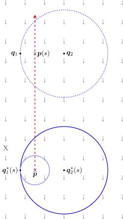
Figure 2.1. Moving the conical point. Shown are the singular support of $\bm{E}^{s}(t,\bm{q}_{1};\bm{q}_{2})=\bm{E}(t,\bm{q}_{1}(s);\bm{q}_{2}(s))$ (solid circles) and the singular support of $\bm{E}(t,\bm{q}_{1};\bm{q}_{2})$ (dotted circles) as the moving conical point $\bm{p}(s)$ travels along the flow of $-\mathbf{X}$; the branch cut is depicted as the red dashed line.

We set $\varphi^{s}=\varphi^{s}_{\mathbf{X}}$ to be the associated flow, the group of local diffeomorphisms given by time-$s$ translation along $\mathbf{X}$. Using $\varphi^{s}$ we assemble the kernel spacetime flow for $\mathbf{X}$, which is the group of locally-defined diffeomorphisms $\Phi^{s}$ on $\mathbb{R}_{t}\times C_{4\pi}^{\circ}\times C_{4\pi}^{\circ}$ given by

$$\Phi^{s}(t,\bm{q}_{1};\bm{q}_{2})\stackrel{{\scriptstyle\textup{def}}}{{=}}\big{(}t,\varphi^{s}(\bm{q}_{1});\varphi^{s}(\bm{q}_{2})\big{)}=\big{(}t,\bm{q}_{1}+s\,\mathbf{X};\bm{q}_{2}+s\,\mathbf{X}\big{)}.$$

Consider the distribution

(2.2) $$\Xi_{s}\stackrel{{\scriptstyle\textup{def}}}{{=}}\chi\partial_{s}\!\left[\big{(}\Phi^{s}\big{)}{}^{*}\,\bm{E}\right],$$

where $\chi=\chi(\bm{q}_{1};\bm{q}_{2})\in\mathcal{C}^{\infty}(C_{4\pi}^{\circ}\times C_{4\pi}^{\circ})$ is a smooth function that vanishes near the cone point. Its role is to ensure that $(\Phi^{s})^{*}\bm{E}$ is well defined on the support of $\chi$; that is, $\chi$ must be chosen so that it vanishes in the set obtained by translating a small ball centered at $\bm{p}$ in the $\mathbf{X}$ direction, and is identically $1$ in a neighbourhood of the set $\{(\bm{q}_{1}+s\mathbf{X},\bm{q}_{2}+s\mathbf{X}):s\in\mathbb{R},(x_{1},x_{2})\in U\}$, where $U$ is a suitably small neighbourhood of $(\bm{q}_{1}^{*},\bm{q}_{2}^{*})$. Then for $(\bm{q}_{1},\bm{q}_{2})\in U$ we have

(2.3) $$\Xi_{s}=\chi\cdot\partial_{s}\!\left[\big{(}\Phi^{s}\big{)}{}^{*}\bm{E}\right]=\partial_{s}\!\left[\big{(}\Phi^{s}\big{)}{}^{*}\bm{E}\right].$$

Set

(2.4) $$\Upsilon_{s}(t,\bm{q}_{1};\bm{q}_{2})\stackrel{{\scriptstyle\textup{def}}}{{=}}\chi(\bm{q}_{1};\bm{q}_{2})\cdot\partial_{s}\!\left[\big{(}\Phi^{s}\big{)}{}^{*}\bm{E}\right]\!(t,\bm{q}_{1};\bm{q}_{2});$$

this is the precise version of the quantity $\frac{d}{ds}\bm{E}^{s}$ in the heuristic discussion above. Thus, we have

(2.5) $$\bm{E}(t,\bm{q}_{1};\bm{q}_{2})=-\int_{0}^{S}\Upsilon_{s}(t,\bm{q}_{1};\bm{q}_{2})\,ds,\quad(\bm{q}_{1},\bm{q}_{2})\in U,$$

provided that $(\Phi^{S})^{*}\bm{E}(t,\bm{q}_{1};\bm{q}_{2})=0$ as discussed above.

When $s=0$, we calculate that

(2.6) $$\Upsilon_{0}(t,\bm{q}_{1};\bm{q}_{2})=\mathbf{X}_{1}\bm{E}(t,\bm{q}_{1};\bm{q}_{2})+\mathbf{X}_{2}\bm{E}(t,\bm{q}_{1};\bm{q}_{2})$$

with $\mathbf{X}_{j}$ denoting $\mathbf{X}$ acting in the $\bm{q}_{j}$-variable, and for general $s$ we have

(2.7) $$\Upsilon_{s}(t,\bm{q}_{1};\bm{q}_{2})=\big{(}\Phi^{s}\big{)}{}^{*}\Upsilon_{0}(t,\bm{q}_{1};\bm{q}_{2}),\quad(\bm{q}_{1},\bm{q}_{2})\in U,$$

since the vector field $\mathbf{X}$ is constant. Pairing $\Upsilon_{0}$ with a test function $\psi\in\mathcal{C}^{\infty}_{\mathrm{c}}(C_{4\pi}^{\circ})$ in the $\bm{q}_{2}$-variable, we then integrate by parts to obtain

$$\left<\Upsilon_{0},\psi\right>_{\bm{q}_{2}} =\left<\mathbf{X}_{1}\bm{E},\psi\right>_{\bm{q}_{2}}+\left<\mathbf{X}_{2}\bm{E},\psi\right>_{\bm{q}_{2}}$$

$$=\left<\mathbf{X}_{1}\bm{E},\psi\right>_{\bm{q}_{2}}-\left<\bm{E},\mathbf{X}\psi\right>_{\bm{q}_{2}}$$

$$=\big{(}\mathbf{X}\circ\mathbf{W}(t)\big{)}\psi-\big{(}\mathbf{W}(t)\circ\mathbf{X}\big{)}\psi$$

$$=\left[\mathbf{X},\mathbf{W}(t)\right]\psi.$$

Thus, $\Upsilon_{0}$ is the Schwartz kernel of the commutator $\left[\mathbf{X},\mathbf{W}(t)\right]$ of the constant vector field with the sine propagator. Note this distribution is everywhere well-defined.

A quick computation now yields the operator identity

$$\text{\qed}\circ\left[\mathbf{X},\mathbf{W}(t)\right]=\left[\mathbf{X},\Delta\right]\circ\mathbf{W}(t),$$

and hence Duhamel’s principle implies

(2.8) $$\left[\mathbf{X},\mathbf{W}(t)\right]=-\int_{s=0}^{t}\mathbf{W}(t-s)\circ\left[\mathbf{X},\Delta\right]\circ\mathbf{W}(s)\,ds,$$

where we recall the Schwartz kernel of these operators is $\Upsilon_{0}$. Using (2.8), we will show that $\Upsilon_{0}$ is a multiple of $\delta(t-r_{1}-r_{2})$, hence a purely diffractive Lagrangian distribution. First, we must understand better the commutator $\left[\mathbf{X},\Delta\right]$. This is the aim of the next subsection.

2.2. Distributions supported at the cone point and commutators

To make full use of the expression (2.8), we need to understand explicitly the Schwartz kernel of the commutator $\left[\mathbf{X},\Delta\right]$. This requires a brief detour through the spectral theory of the Laplacian on $C_{4\pi}$, and, in particular, a discussion of the failure of essential self-adjointness of the Laplace-Beltrami operator $\Delta_{g}$ on $C^{\circ}_{4\pi}$.

Let $H^{s}(C_{4\pi})$ denote the usual Sobolev spaces on $C_{4\pi}$, defined as

(2.9) $$H^{k}(C_{4\pi})\stackrel{{\scriptstyle\textup{def}}}{{=}}\left\{u\in L^{2}(C_{4\pi}):\operatorname{Diff}^{k}(C_{4\pi})\cdot u\in L^{2}(C_{4\pi})\right\}$$

for integers $k\in\mathbb{Z}_{\geqslant 0}$ and extended to all real orders by duality and interpolation. An exercise (essentially the same as a more standard calculation on $\mathbb{R}^{2}$, where the same result holds; cf. Chapter I.5 of [AGHKH]) shows that the closure of $\mathcal{C}^{\infty}_{\mathrm{c}}(C_{4\pi}^{\circ})$ in the graph norm for $\Delta_{g}$,

$$\|u\|_{\Delta_{g}}\stackrel{{\scriptstyle\textup{def}}}{{=}}\|u\|_{L^{2}}+\|\Delta_{g}u\|_{L^{2}},$$

i.e., the domain of the closure $\overline{\Delta_{g}}$ of $\Delta_{g}$, is

(2.10) $$\overline{\mathfrak{D}}\stackrel{{\scriptstyle\textup{def}}}{{=}}\operatorname{Dom}\!\left(\overline{\Delta_{g}}\right)=\left\{u\in H^{2}(C_{4\pi}):u(\bm{p})=0\right\}.$$

Thus, if $\rho\in\mathcal{C}^{\infty}_{\mathrm{c}}(C_{4\pi})$ is any bump function satisfying $\rho\equiv 1$ for $r\leqslant 1$ and $\rho\equiv 0$ for $r\geqslant 2$, then this shows

$$H^{2}(C_{4\pi})=\overline{\mathfrak{D}}\oplus\mathrm{Span}_{\mathbb{C}}\{\rho\}.$$

We show in Lemma A.1 that the domain of the adjoint of this operator is

$$\overline{\mathfrak{D}}{}^{*}\stackrel{{\scriptstyle\textup{def}}}{{=}}\operatorname{Dom}\!\left(\overline{\Delta_{g}}{}^{*}\right)=\overline{\mathfrak{D}}\oplus\mathrm{Span}_{\mathbb{C}}\!\left\{\rho,\rho\log(r),\rho\,r^{\frac{1}{2}}\exp\!\left[\pm\frac{i}{2}\theta\right],\rho\,r^{-\frac{1}{2}}\exp\!\left[\pm\frac{i}{2}\theta\right]\right\}.$$

The choice of a self-adjoint extension of $\overline{\Delta_{g}}$ is then the suitable choice of a half-dimensional subspace of $\overline{\mathfrak{D}}{}^{*}\big{/}\overline{\mathfrak{D}}$ (cf. [ReeSim2] for more details on self-adjoint extensions).

In our analysis, we have elected to work with the Friedrichs extension $\Delta\stackrel{{\scriptstyle\textup{def}}}{{=}}\Delta_{g}^{\mathrm{Fr}}$ of the Laplacian, the unique self-adjoint extension whose domain contains the form domain (which in our setting is $H^{1}(C_{4\pi})$). We define the spaces $\mathcal{D}_{s}$ to be the domains of real powers of this operator:

(2.11) $$\mathcal{D}_{s}\stackrel{{\scriptstyle\textup{def}}}{{=}}\operatorname{Dom}\!\left(\Delta^{\frac{s}{2}}\right).$$

For $s>1$, these spaces are strictly larger than the Sobolev spaces $H^{s}(C_{4\pi})$. In particular, $\mathcal{D}_{2}$ is the Friedrichs domain itself.

To distinguish the elements of $\mathcal{D}_{2}$ from those of $\overline{\mathfrak{D}}$, we must examine their behavior at $\bm{p}$. We do so in the following lemma, which we prove in Appendix A.

Lemma 2.1.

Fix a compactly supported, smooth, and radial cutoff $\rho\in\mathcal{C}^{\infty}_{\mathrm{c}}(C_{4\pi})$ which is identically $1$ near $\bm{p}$. For any function $u\in\mathcal{D}_{2}$, there exist constants $a_{-1}$, $a_{0}$, and $a_{1}$ in $\mathbb{C}$ and a distribution $v\in\overline{\mathfrak{D}}$ such that

(2.12) $$u=\left(a_{0}+a_{-1}\sqrt{r}\,\exp\!\left[-\frac{i}{2}\,\theta\right]+a_{1}\sqrt{r}\,\exp\!\left[\frac{i}{2}\,\theta\right]\right)\rho(r)+v.$$

In particular, the function $u-a_{0}-a_{-1}\sqrt{r}\,\exp\!\left[-\frac{i}{2}\,\theta\right]-a_{1}\sqrt{r}\,\exp\!\left[\frac{i}{2}\,\theta\right]$ vanishes at $\bm{p}$.

Remark 2.2.

We see from Lemma 2.1 the system of strict inclusions

$$\overline{\mathfrak{D}}\subsetneq H^{2}(C_{4\pi})\subsetneq\mathcal{D}_{2}\subsetneq\overline{\mathfrak{D}}{}^{*}.$$

Using this lemma, we see that the Friedrichs extension exactly corresponds to the choice of the functions

$$\varphi_{0}(r,\theta)\stackrel{{\scriptstyle\textup{def}}}{{=}}1,\quad\varphi_{-1}(r,\theta)\stackrel{{\scriptstyle\textup{def}}}{{=}}\sqrt{r}\exp\!\left[-\frac{i}{2}\,\theta\right],\quad\text{and}\quad\varphi_{+1}(r,\theta)\stackrel{{\scriptstyle\textup{def}}}{{=}}\sqrt{r}\exp\!\left[\frac{i}{2}\theta\right]$$

as the models for the admissible asymptotics at $\bm{p}$. Given a function $u$ in $\mathcal{D}_{2}$, we define the distributions $L_{j}$ for $j=-1$, $0$, or $+1$ as

(2.13) $$L_{j}(u)\stackrel{{\scriptstyle\textup{def}}}{{=}}a_{j}$$

in terms of the expansion (2.12). Note that the expansion (2.12) is independent of the choice of the cutoff $\rho$, for the difference of any two such cutoffs is compactly supported in $C^{\circ}_{4\pi}$ and is thus in $\overline{\mathfrak{D}}$. Hence, the distributions $L_{j}$ are well-defined elements of $\overline{\mathfrak{D}}_{-2}$. Equivalently, we may define the $L_{j}$’s using the angular spectral projectors

(2.14) $$\left[\Pi_{j}u\right]\!(r)\stackrel{{\scriptstyle\textup{def}}}{{=}}\frac{1}{\sqrt{4\pi}}\int_{\mathbb{R}/4\pi\mathbb{Z}}u(r,\theta)\,\exp\!\left[-\frac{ij}{2}\,\theta\right]d\theta,$$

and a straightforward computation shows that

(2.15) $$L_{0}(u)=\frac{1}{\sqrt{4\pi}}\lim_{r\downarrow 0}\big{[}\Pi_{0}u\big{]}(r)\quad\text{and}\quad L_{\pm 1}(u)=\frac{1}{\sqrt{4\pi}}\lim_{r\downarrow 0}\frac{\big{[}\Pi_{\pm 1}u\big{]}(r)}{\sqrt{r}}.$$

Directly from the definition or from the above, we observe that $L_{\pm 1}(u)=\overline{L_{\mp 1}(\overline{u})}$.

Corollary 2.3.

Suppose $L$ is a distribution in $\mathcal{D}_{-2}$ which is supported only at the cone point $\bm{p}$. Then $L$ is a linear combination of $L_{-1}$, $L_{0}$, and $L_{1}$.

Proof.

Suppose $u$ is an element of $\mathcal{D}_{2}$. By (2.12) we have

$$L(u)=a_{0}\,L\big{(}\rho(r)\big{)}+a_{-1}\,L\big{(}\varphi_{-1}(r,\theta)\cdot\rho(r)\big{)}+a_{1}\,L\big{(}\varphi_{1}(r,\theta)\cdot\rho(r)\big{)}$$

since $v$ being an element of $\overline{\mathfrak{D}}$ implies $L(v)$ vanishes. Therefore,

$$L=L\big{(}\rho(r)\big{)}\cdot L_{0}+L\big{(}\varphi_{-1}(r,\theta)\cdot\rho(r)\big{)}\cdot L_{-1}+L\big{(}\varphi_{1}(r,\theta)\cdot\rho(r)\big{)}\cdot L_{1},$$

showing that $u$ is a linear combination of $L_{0}$, $L_{-1}$, and $L_{1}$ as claimed. ∎

Returning to the commutator $\left[\mathbf{X},\Delta\right]$, let us observe

$$\mathbf{X}:\mathcal{D}_{2}\centernot\longrightarrow\mathcal{D}_{1}=H^{1}(C_{4\pi})$$

since $\mathcal{D}_{2}$ is not contained in $H^{2}(C_{4\pi})$. On the other hand, since $H^{1}(C_{4\pi})$ is contained in $\mathcal{D}_{2}$, we certainly have $\mathbf{X}:\mathcal{D}_{2}\to L^{2}(C_{4\pi})$, and hence, by duality, also $\mathbf{X}:L^{2}(C_{4\pi})\to\mathcal{D}_{-2}$. Therefore, for any $u\in\mathcal{D}_{2}$, the commutator $\left[\mathbf{X},\Delta\right]$ is in $\mathcal{D}_{-2}$. On the other hand, if $u$ is compactly supported in $C_{4\pi}^{\circ}$, then the action of $\Delta$ on $u$ is the same as the Euclidean Laplacian acting on $u$. Since the Euclidean Laplacian commutes with constant vector fields, this implies $\left[\mathbf{X},\Delta\right]u=0$. Therefore, the distributional support of $\left[\mathbf{X},\Delta\right]u$ for any $u\in\mathcal{D}_{2}$ is at most the cone point $\bm{p}$, and thus it fits into the framework of Corollary 2.3.

Proposition 2.4.

Let $\mathbf{X}=X_{w}\,\partial_{w}+X_{\overline{w}}\,\partial_{\overline{w}}$ be a constant vector field on $C_{4\pi}$, written in terms of the complex coordinate $w=x+iy=re^{i\theta}$. Then for any distribution $u\in\mathcal{D}_{k}$ for $k\geqslant 2$, we have

(2.16) $$\left[\mathbf{X},\Delta\right]u=-2\pi\big{(}X_{w}\,L_{1}(u)\cdot L_{1}+X_{\overline{w}}\,L_{-1}(u)\cdot L_{-1}\big{)}$$

Proof.

Consider the bilinear pairing

$$\big{\langle}[\mathbf{X},\Delta]u,v\big{\rangle},\quad u,v\in\mathcal{D}_{2}.$$

The discussion above shows that this is well defined for all $u,v\in\mathcal{D}_{2}$. It is clear that this pairing vanishes if either $u$ or $v$ lie in $\overline{\mathfrak{D}}$. So to compute the pairing, it suffices to consider $u$ and $v$ to be linear combinations of the functions $\zeta_{0}=\rho(|w|^{2})$, $\zeta_{-1}(w)\stackrel{{\scriptstyle\textup{def}}}{{=}}{\overline{w}}^{\frac{1}{2}}\,\rho(|w|^{2})$ and $\zeta_{1}(w)\stackrel{{\scriptstyle\textup{def}}}{{=}}w^{\frac{1}{2}}\,\rho(|w|^{2})$. In fact, the pairing also vanishes if either $u$ or $v$ are $\zeta_{0}$ since this is equal to a constant in a neighbourhood of the cone point, hence vanishes near the cone point after the application of either $\mathbf{X}$ or $\Delta$. So we need only consider $u$ and $v$ equal to a combination of $\zeta_{\pm 1}$.

First, let $\mathbf{X}=\partial_{w}$. For this $\mathbf{X}$, consider the action of the operator $[\mathbf{X},\Delta]$ on a Fourier mode $e^{ij\theta}$, for a half-integer $j$. Since the Fourier modes are eigenfunctions of $\Delta_{\mathbb{S}^{1}_{4\pi}}$, and since $\partial_{w}$ maps $e^{ij\theta}$ to a multiple of $e^{i(j-1)\theta}$, the same property is true of $[\mathbf{X},\Delta]$. It follows that the only nonzero combination with $\mathbf{X}=\partial_{w}$ is

$$\big{\langle}[\partial_{w},\Delta]\zeta_{1},\zeta_{1}\big{\rangle}.$$

Similarly, when $\mathbf{X}=\partial_{\overline{w}}$, the only nonzero combination occurs when $u=v=\zeta_{-1}$. In view of these considerations, to establish (2.16), it suffices to show that

(2.17) $$\big{\langle}[\partial_{w},\Delta]\zeta_{1},\zeta_{1}\big{\rangle} =-2\pi,$$

$$\big{\langle}[\partial_{\overline{w}},\Delta]\zeta_{-1},\zeta_{-1}\big{\rangle} =-2\pi.$$

In fact, as the calculations are similar, we only prove the first.

Since we are using the bilinear pairing we have

$$\big{\langle}[\partial_{w},\Delta]\zeta_{1},\zeta_{1}\big{\rangle}=-2\big{\langle}\Delta\zeta_{1},\partial_{w}\zeta_{1}\big{\rangle}=-2\int_{C_{4\pi}}\Delta\zeta_{1}\partial_{w}\zeta_{1}\,dS$$

where $dS$ denotes the Euclidean area element. Using Stokes formula we have:

$$\int_{r=\varepsilon}(\partial_{w}\zeta_{1})^{2}\,dw=i\int_{r\geq\varepsilon}\Delta\zeta_{1}\partial_{w}\zeta_{1}\,dS.$$

For $\varepsilon$ small enough we thus obtain

$$\int_{r\geq\varepsilon}\Delta\zeta_{1}\partial_{w}\zeta_{1}\,dS=\pi.$$

The claim follows. ∎

2.3. The differentiated wave propagator on $C_{4\pi}$

We now apply the formula (2.16) for the Schwartz kernel of the commutator $\left[\mathbf{X},\Delta\right]$ to the Duhamel formula (2.8) to compute the distribution $\Upsilon_{0}$. Writing $\mathbf{X}$ in complex coordinates, i.e., $\mathbf{X}=X_{w}\,\partial_{w}+X_{{\overline{w}}}\,\partial_{{\overline{w}}}$, this yields

(2.18) $$\Upsilon_{0}(t,\bm{q}_{1};\bm{q}_{2})=2\pi\int_{s=0}^{t}\Big{\{}X_{w}\big{[}\mathbf{W}(t-s)L_{1}\big{]}(\bm{q}_{1})\cdot\big{[}L_{1}\circ\mathbf{W}(s)\big{]}(\bm{q}_{2})\\ \mbox{}+X_{{\overline{w}}}\big{[}\mathbf{W}(t-s)L_{-1}\big{]}(\bm{q}_{1})\cdot\big{[}L_{-1}\circ\mathbf{W}(s)\big{]}(\bm{q}_{2})\Big{\}}\,ds.$$

In particular, this shows $\Upsilon_{0}$ is an integral superposition of tensor products of the distributions

(2.19) $$\ell_{j}(t)\stackrel{{\scriptstyle\textup{def}}}{{=}}\mathbf{W}(t)\,L_{j}$$

obtained from evolving the distributions $L_{j}$ under the sine flow $\mathbf{W}(t)$. (Note that the self-adjointness of $\mathbf{W}(t)$, and the fact that its kernel is real, implies $\mathbf{W}(t)\,L_{j}=L_{j}\circ\mathbf{W}(t)$, so we only need to work with the evolved distributions $\ell_{j}(t)$.) Since the $L_{j}$’s are supported only at the cone point $\bm{p}$, we should expect the propagated distributions $\ell_{j}(t)$ to be spherical waves emanating out from $\bm{p}$, i.e., they should be diffractive-type waves. As the next lemma shows, this is indeed the case.

Lemma 2.5.

Let $t>0$. The distributions $\ell_{1}(t)$ and $\ell_{-1}(t)$ on $C_{4\pi}$ are given explicitly by

(2.20) $$\ell_{\pm 1}(t)=\frac{1}{4\pi\sqrt{r}}\delta(t-r)\exp\!\left[\mp\frac{i}{2}\,\theta\right].$$

Proof of Lemma 2.5.

It suffices to prove the lemma for $\ell_{1}(t)$; the statement for $\ell_{-1}(t)$ is similar and follows by complex conjugation.

Recall the spectral projector form of the definition of $L_{1}$ (see (2.15) and (2.14)) and

$$L_{1}(u)=\lim_{r\downarrow 0}\frac{1}{4\pi\sqrt{r}}\int_{\mathbb{R}/4\pi\mathbb{Z}}u(r,\theta)\,\exp\!\left[-\frac{i}{2}\theta\right]d\theta.$$

To compute the action of $\mathbf{W}(t)$ on $L_{1}$, we use Cheeger’s functional calculus on metric cones [CheTay1]; this expresses $\bm{E}$ as the sum

$$\bm{E}(t,r_{1},\theta_{1};r_{2},\theta_{2})=\frac{1}{4\pi}\sum_{j\in\mathbb{Z}}\exp\!\left[\frac{ij}{2}\,(\theta_{1}-\theta_{2})\right]\int_{\lambda=0}^{\infty}\frac{\sin(\lambda t)}{\lambda}\,J_{\frac{|j|}{2}}(\lambda r_{1})\,J_{\frac{|j|}{2}}(\lambda r_{2})\,\lambda\,d\lambda$$

over the angular modes of $\Delta$. Since $L_{1}$ vanishes except at the $j=1$ mode in this sum, we have the following simple formula for the action of $\ell_{1}(t)$.

$$\big{[}\ell_{1}(t)\big{]}(u)\\ \mbox{}=\lim_{r_{1}\downarrow 0}\frac{1}{(4\pi)^{2}\sqrt{r_{1}}}\int_{\theta_{1}=0}^{4\pi}\int_{r_{2}=0}^{\infty}\int_{\theta_{2}=0}^{4\pi}\left\{\int_{\lambda=0}^{\infty}\frac{\sin(\lambda t)}{\lambda}\,J_{\frac{1}{2}}(\lambda r_{1})\,J_{\frac{1}{2}}(\lambda r_{2})\,\lambda\,d\lambda\right\}\\ \mbox{}\times\exp\!\left[-\frac{i}{2}\,\theta_{1}\right]\exp\!\left[\frac{i}{2}(\theta_{1}-\theta_{2})\right]u(r_{2},\theta_{2})\,d\theta_{1}\,r_{2}\,dr_{2}d\theta_{2}$$

Performing the $\theta_{1}$-integral, this simplifies to

$$\big{[}\ell_{1}(t)\big{]}(u)=\lim_{r_{1}\downarrow 0}\frac{1}{4\pi\sqrt{r_{1}}}\int_{r_{2}=0}^{\infty}\int_{\theta_{2}=0}^{4\pi}\left\{\int_{\lambda=0}^{\infty}\frac{\sin(\lambda t)}{\lambda}\,J_{\frac{1}{2}}(\lambda r_{1})\,J_{\frac{1}{2}}(\lambda r_{2})\,\lambda\,d\lambda\right\}\\ \mbox{}\times\exp\!\left[-\frac{i}{2}\,\theta_{2}\right]u(r_{2},\theta_{2})\,r_{2}\,dr_{2}d\theta_{2}.$$

We now substitute the explicit formula $J_{\frac{1}{2}}(z)=\left[\frac{2}{\pi z}\right]^{\frac{1}{2}}\sin(z)$ into the above, giving

$$\ell_{1}(t)=\lim_{r_{1}\downarrow 0}\frac{1}{2\pi^{2}\sqrt{r_{2}}}\int_{\lambda=0}^{\infty}\sin(\lambda t)\,\frac{\sin(\lambda r_{1})}{\lambda r_{1}}\,\sin(\lambda r_{2})\,\exp\!\left[-\frac{i}{2}\theta_{2}\right]\,d\lambda.$$

By pairing with a test function and using dominated convergence, we see that this is equivalent (in the sense of distributions) to the expression

$$\ell_{1}(t)=\frac{1}{2\pi^{2}\sqrt{r_{2}}}\int_{\lambda=0}^{\infty}\sin(\lambda t)\sin(\lambda r_{2})\exp\!\left[-\frac{i}{2}\theta_{2}\right]d\lambda.$$

To conclude the proof, we observe

$$\int_{\lambda=0}^{\infty}e^{-i\lambda(t+r)}\,d\lambda=\int_{\lambda=-\infty}^{0}e^{i\lambda(t+r)}\,d\lambda.$$

This implies, dropping the subscripts from the base variables and replacing the sine functions by their complex exponential definitions, that

(2.21) $$\begin{gathered}\ell_{1}(t)=-\frac{1}{8\pi^{2}\sqrt{r}}\int_{\lambda=-\infty}^{\infty}\left\{e^{i\lambda(t+r)}-e^{i\lambda(t-r)}\right\}\exp\!\left[-\frac{i}{2}\,\theta\right]d\lambda\\ =\frac{1}{4\pi\sqrt{r}}\delta(t-r)\exp\!\left[-\frac{i}{2}\,\theta\right],\text{ for }t>0.\end{gathered}$$

∎

Remark 2.6.

It is remarkable that, on the cone of angle $4\pi$, there are solutions to the wave equation, namely $r^{-\frac{1}{2}}\delta(t-r)e^{\pm i\theta/2}$ obeying the sharp Huygen’s principle, that is, supported on the light cone itself. This can be confirmed by direct calculation, applying the wave operator to these distributions.

We also remark that one can prove Lemma 2.5 without appealing to the Cheeger functional calculus: after verifying that the $\ell_{\pm}(t)$ satisfy the wave equation, it only remains to check that $\lim_{t\to 0}\ell_{\pm 1}(t)=0$ and $\lim_{t\to 0}(d/dt)\ell_{\pm 1}(t)=L_{\pm 1}$.

We conclude this subsection with the proof that $\Upsilon_{0}$ is a Lagrangian distribution associated to the diffractive Lagrangian relation $\Lambda^{\bm{\mathsf{D}}}$.

Proposition 2.7.

Let $t>0$, and suppose, as in the discussion in Section 2.1, that $\mathbf{X}$ points in the direction $\theta$. Then the distribution $\Upsilon_{0}=\mathcal{K}\big{[}\left[\mathbf{X},\mathbf{W}(t)\right]\big{]}$ is given explicitly in polar coordinates by

(2.22) $$\Upsilon_{0}(t,\bm{q}_{1};\bm{q}_{2})=\frac{1}{4\pi\sqrt{r_{1}r_{2}}}\delta(t-r_{1}-r_{2})\cos\!\left(\frac{\theta_{1}+\theta_{2}}{2}-\theta\right).$$

Proof.

We begin by rewriting the equation (2.18) using the distributions $\ell_{j}(t)$:

$$\Upsilon_{0}(t,\bm{q}_{1};\bm{q}_{2})=2\pi\int_{s=0}^{t}\Big{\{}X_{w}\,\big{[}\ell_{1}(t-s)\big{]}(\bm{q}_{1})\cdot\big{[}\ell_{1}(s)\big{]}(\bm{q}_{2})\\ \mbox{}+X_{{\overline{w}}}\,\big{[}\ell_{-1}(t-s)\big{]}(\bm{q}_{1})\cdot\big{[}\ell_{-1}(s)\big{]}(\bm{q}_{2})\Big{\}}\,ds.$$

We break up the integral across the sum and consider the first summand:

$$\Upsilon_{0}^{w}(t,\bm{q}_{1};\bm{q}_{2})\stackrel{{\scriptstyle\textup{def}}}{{=}}\int_{s=0}^{t}\big{[}\ell_{1}(t-s)\big{]}(\bm{q}_{1})\cdot\big{[}\ell_{1}(s)\big{]}(\bm{q}_{2})\,ds.$$

Substituting our expression (2.21) in for $\ell_{1}(t)$ and its conjugate for $\ell_{-1}(t)$, the above becomes

(2.23) $$\begin{gathered}\frac{1}{16\pi^{2}\sqrt{r_{1}r_{2}}}\int_{s=0}^{t}\delta((t-s)-r_{1})\delta(s-r_{2})\exp\!\left[-\frac{i}{2}\,(\theta_{1}+\theta_{2})\right]\,ds\\ =\frac{1}{16\pi^{2}\sqrt{r_{1}r_{2}}}\delta(t-r_{1}-r_{2})\exp\!\left[-\frac{i}{2}\,(\theta_{1}+\theta_{2})\right].\end{gathered}$$

Similarly, we have

(2.24) $$\Upsilon_{0}^{{\overline{w}}}(t,\bm{q}_{1};\bm{q}_{2})=\frac{1}{16\pi^{2}\sqrt{r_{1}r_{2}}}\delta(t-r_{1}-r_{2})\exp\!\left[\frac{i}{2}\,(\theta_{1}+\theta_{2})\right].$$

For the vector field with direction $\theta$, we have $X_{w}=\exp(i\theta)=\overline{X_{{\overline{w}}}}$. Adding (2.23) times $X_{w}$ to (2.24) times $X_{{\overline{w}}}$, and multiplying by $2\pi$, we obtain (2.22). ∎

2.4. The full wave propagator on $C_{4\pi}$

Having computed $\Upsilon_{0}(t,\bm{q}_{1};\bm{q}_{2})$, we return to (2.5) and compute the sine wave kernel $\bm{E}(t,\bm{q}_{1},\bm{q}_{2})$ on $C_{4\pi}$. Since our primary interest is in the behaviour near a geometric diffractive geodesic, let us assume for a while that $\theta_{1}$ is close to $0$ and $\theta_{2}$ is close to $\pi$ (so that the diffraction angle $\theta_{1}-\theta_{2}$ is close to $-\pi$). We then choose to move the conical point in the direction $\frac{\pi}{2}.$ This amounts to putting $\theta=-\frac{\pi}{2}$ in the previous formulas.

Let $r_{j}(s),\theta_{j}(s)$ be the distance and angle from the point $\bm{q}_{j}$ to the cone point shifted by a distance $s$ in the $\theta=\frac{\pi}{2}$ direction, or equivalently, from the point $\bm{q}_{j}(s)$, obtained from $\bm{q}_{j}$ by shifting a distance $s$ in the $\theta=-\frac{\pi}{2}$ direction, to the (fixed) cone point. Notice that, in the limit $s\to\infty$, the angle between $\bm{q}_{1}(s)$ and $\bm{q}_{2}(s)$ approaches $2\pi$. In particular, the points will be distance $r_{1}(s)+r_{2}(s)=2s+O(1)$ apart, in this limit. Thus, the condition that $(\Phi^{s})^{*}\bm{E}(t,\bm{q}_{1};\bm{q}_{2})=0$ is valid for large $s$. Hence, we can write, using (2.23) and (2.5),

(2.25) $$\bm{E}(t,\bm{q}_{1},\bm{q}_{2})=\frac{1}{4\pi}\int_{0}^{\infty}(r_{1}(s)r_{2}(s))^{-\frac{1}{2}}\delta(t-r_{1}(s)-r_{2}(s))\sin\!\left(\frac{\theta_{1}(s)+\theta_{2}(s)}{2}\right)ds.$$

This can be written

(2.26) $$\bm{E}(t,\bm{q}_{1};\bm{q}_{2})=\int_{s\geq 0}\int_{-\infty}^{\infty}e^{i\phi(t,\bm{q}_{1},\bm{q}_{2},s,\omega)}a(t,\bm{q}_{1},\bm{q}_{2},s,\omega)\,ds\,d\omega$$

with the following phase function and amplitude:

(2.27) $$\phi(\bm{q}_{1},\bm{q}_{2},s,\omega) =\Big{(}\sqrt{x_{1}^{2}+(y_{1}-s)^{2}}+\sqrt{x_{2}^{2}+(y_{2}-s)^{2}}-t\Big{)}\omega,$$

$$a(t,\bm{q}_{1},\bm{q}_{2},s,\omega) =\frac{1}{8\pi^{2}}\cdot\big{(}r_{1}(s)r_{2}(s)\big{)}^{-\frac{1}{2}}\cdot\sin\!\left(\frac{\theta_{1}(s)+\theta_{2}(s)}{2}\right).$$

Since the phase function is a nondegenerate phase function in the sense of Definition 1.3, we find that the propagator is in the Melrose-Uhlmann class.

This construction can actually be carried out as long as $\theta_{1}\in(-\frac{\pi}{2},\frac{\pi}{2})$ and $\theta_{2}\in(\frac{\pi}{2},\frac{3\pi}{2}).$ When $\theta_{1}$ is in the same interval but $\theta_{2}$ now belongs to $(-\frac{3\pi}{2},-\frac{\pi}{2})$ (thus containing the diffraction angle of $+\pi$), the conical point have to be moved in the opposite direction $\theta=-\frac{\pi}{2}.$ This leads to a similar expression. Observe however that in that case the phase is now

$$\phi(\bm{q}_{1},\bm{q}_{2},s,\omega)=\Big{(}\sqrt{x_{1}^{2}+(y_{1}+s)^{2}}+\sqrt{x_{2}^{2}+(y_{2}+s)^{2}}-t\Big{)}\omega,$$

In the remaining cases for which $\theta_{2}$ belongs respectively to $(-\frac{\pi}{2},\frac{\pi}{2})$ and $(\frac{3\pi}{2},\frac{5\pi}{2})$ the conical point can be moved in the $\theta=\pi$ direction. It should be noted however that in this case the limit $s\rightarrow\infty$ of $\bm{E}^{s}(t,\bm{q}_{1},\bm{q}_{2})$ is not $0$ but the free solution.

In any case, it follows that $\bm{E}$ is an intersecting Lagrangian distribution in a neighbourhood of $(t,\bm{q}_{1};\bm{q}_{2})$. Close to the diffraction angle $-\pi$, we use the form of the phase (2.27) to determine the two Lagrangian submanifolds. First, when $s=0$, it is clear that $\phi|_{s=0}$ parametrizes the Lagrangian $N^{*}\{t=r_{1}+r_{2}\}=\Lambda^{\bm{\mathsf{D}}}$. Second, when $s=0$, $\phi$ is stationary with respect to $s$ when the cone point lies on the straight line between $(x_{1},y_{1}+s)$ and $(x_{2},y_{2}+s)$. In this case, the second derivative $\partial^{2}_{ss}\phi$ is nonzero, and we can eliminate the variable $s$ by replacing it with its stationary value. In this case, the sum of distances $\sqrt{x_{1}^{2}+(y_{1}+s)^{2}}+\sqrt{x_{2}^{2}+(y_{2}+s)^{2}}$ is equal to the distance between $(x_{1},y_{1}+s)$ and $(x_{2},y_{2}+s)$, which is the same as the distance between $\bm{q}_{1}$ and $\bm{q}_{2}$. So an equivalent phase function is $(|\bm{q}_{1}-\bm{q}_{2}|-t)\omega$, and this parametrizes the conormal bundle of the direct front, $\Lambda^{\bm{\mathsf{G}}}$.

This essentially proves

Proposition 2.8.

For each fixed $t>0$, the sine propagator kernel $\bm{E}$ on $C_{4\pi}$ is an intersecting Lagrangian distribution on $C_{4\pi}^{\circ}\times C_{4\pi}^{\circ}$ of order $-1$:

$$\bm{E}(t)\in r_{1}^{-\frac{1}{2}}\,r_{2}^{-\frac{1}{2}}\cdot I^{-1}\!\left(C_{4\pi}^{\circ}\times C_{4\pi}^{\circ};\Lambda^{\bm{\mathsf{D}}},\Lambda^{\bm{\mathsf{G}}}\right);$$

in particular, it has Lagrangian order $-1$ on $\Lambda^{\bm{\mathsf{G}}}\setminus\Lambda^{\bm{\mathsf{D}}}$ and order $-\frac{3}{2}$ on $\Lambda^{\bm{\mathsf{D}}}\setminus\Lambda^{\bm{\mathsf{G}}}$.

2.5. The Cheeger-Taylor formula

It is instructive to compute the integral (2.25) explicitly, and confirm that we obtain the Cheeger-Taylor formulae for the wave kernel from Section 2.1. Let us consider the case in which $\theta_{1}\in(-\frac{\pi}{2},\frac{\pi}{2})$ and $\theta_{2}\in(\frac{\pi}{2},\frac{3\pi}{2})$

Since the functions $r_{i}(s)$ take the form $\sqrt{r_{0}^{2}+(s-s_{0})^{2}}$, they are convex functions of $s$. Therefore, as $s$ ranges from $0$ to $\infty$, the delta function $\delta(t-r_{1}(s)-r_{2}(s))$ can be nonzero for at most two values of $s$. More precisely, if $t<r_{1}+r_{2}$ and the angle between $\bm{q}_{1}$ and $\bm{q}_{2}$ is greater than $\pi$, then there are no values of $s$ for which $t=r_{1}(s)+r_{2}(s)$, since in this case, both $r_{1}(s)$ and $r_{2}(s)$ are increasing in $s$. On the other hand, suppose that $t<r_{1}+r_{2}$ and the angle between $x_{1}$ and $x_{2}$ is less than $\pi$. We might as well assume that $t>d(x_{1},x_{2})$, since otherwise the wave kernel is zero due to finite speed of propagation. In this case, $r_{1}(s)+r_{2}(s)$ decreases until the cone point lies directly between $x_{1}$ and $x_{2}$, when we have $r_{1}(s)+r_{2}(s)=d(x_{1},x_{2})<t$, and then increases to infinity. It follows that in this case there are two values of $s$ for which $t=r_{1}(s)+r_{2}(s)$. The final case is $t>r_{1}+r_{2}$. In this case, regardless of whether $r_{1}(s)+r_{2}(s)$ initially increases or decreases, there is always one value of $s$ for which $t=r_{1}(s)+r_{2}(s)$.

For each value of $s$ satisfying $t=r_{1}(s)+r_{2}(s)$, we calculate the contribution to the integral (2.25). This is given by

(2.28) $$\frac{1}{4\pi}(r_{1}(s)r_{2}(s))^{-\frac{1}{2}}\big{|}r_{1}^{\prime}(s)+r^{\prime}_{2}(s)\big{|}^{-1}\sin\!\left(\frac{\theta_{1}(s)+\theta_{2}(s)}{2}\right)\\ =\frac{1}{4\pi}(r_{1}(s)r_{2}(s))^{-\frac{1}{2}}\left|\sin\!\left(\theta_{1}(s)\right)+\sin\!\left(\theta_{2}(s)\right)\right|^{-1}\sin\!\left(\frac{\theta_{1}(s)+\theta_{2}(s)}{2}\right)\\ =\frac{1}{4\pi}\left[(r_{1}(s)r_{2}(s)\right]^{-\frac{1}{2}}\left|\frac{\sin\!\left(\frac{\theta_{1}(s)+\theta_{2}(s)}{2}\right)}{\sin\!\left(\theta_{1}(s)\right)+\sin\!\left(\theta_{2}(s)\right)}\right|,$$

since by choice $\frac{\theta_{1}(s)+\theta_{2}(s)}{2}\in(0,\pi).$ Using the addition formula for $\sin\theta_{1}+\sin\theta_{2}$ we obtain that the contribution can be written

$$\frac{1}{8\pi}(r_{1}(s)r_{2}(s))^{-\frac{1}{2}}\left|\cos\!\left(\frac{\theta_{1}-\theta_{2}}{2}\right)\right|^{-1}$$

and we want to prove that this coincides with

$$\frac{1}{4\pi}\Big{(}t^{2}-\big{(}r_{1}^{2}+r_{2}^{2}-2r_{1}r_{2}\cos(\theta_{1}-\theta_{2})\big{)}\Big{)}^{-\frac{1}{2}},$$

whenever the moved conical point $\bm{p}(s)$ lies in between $\bm{q}_{1}$ and $\bm{q}_{2}.$ This implies that $t=r_{1}(s)+r_{2}(s)$ so that we have (we omit the dependence on $s$)

(2.29) $$t^{2}-\big{(}r_{1}^{2}+r_{2}^{2}-2r_{1}r_{2}\cos(\theta_{1}-\theta_{2})\big{)}\\ \mbox{}=2r_{1}r_{2}\big{(}1+\cos(\theta_{1}-\theta_{2})\big{)}=4r_{1}r_{2}\cos^{2}\!\left(\frac{\theta_{1}-\theta_{2}}{2}\right).$$

The claim thus follows.

The wave kernel on $C_{4\pi}$ is therefore given by $0$, $1$ or $2$ times this quantity, according as there are $0$, $1$ or $2$ values of $s>0$ satisfying $t=r_{1}(s)+r_{2}(s)$, as discussed above. This agrees with the expression (2.1a)–(2.1c) obtained by Cheeger-Taylor.

3. The microlocal structure of the wave propagator on $C_{\alpha}$

We now analyze the structure of the Schwartz kernel $\bm{E}$ of the sine propagator on the cone $C_{\alpha}$ of generic cone angle $\alpha$. First let us recall the definitions of the geometric and diffractive Lagrangians and their intersection: the geometric (or “main”) Lagrangian is

(3.1a) $$\Lambda^{\bm{\mathsf{G}}}\stackrel{{\scriptstyle\textup{def}}}{{=}}N^{*}\!\left\{t^{2}=r_{1}^{2}+r_{2}^{2}-2r_{1}r_{2}\cos(\theta_{1}-\theta_{2})\text{ and }|\theta_{1}-\theta_{2}|\leqslant\pi\right\},$$

the diffractive Lagrangian is

(3.1b) $$\Lambda^{\bm{\mathsf{D}}}\stackrel{{\scriptstyle\textup{def}}}{{=}}N^{*}\!\left\{t^{2}=\left(r_{1}+r_{2}\right)^{2}\right\},$$

and their intersection is the singular set

(3.1c) $$\Sigma\stackrel{{\scriptstyle\textup{def}}}{{=}}\Lambda^{\bm{\mathsf{G}}}\cap\Lambda^{\bm{\mathsf{D}}}$$

In particular, we note that $\operatorname{pr}(\Sigma)=\left\{\text{$t^{2}=(r_{1}+r_{2})^{2}$ and $\theta_{1}-\theta_{2}=\pm\pi$}\right\}$.

To do this, we use Friedlander’s representation of the sine wave kernel $\bm{E}(t)$ on the cone of angle $\alpha$, which expresses, in effect, this wave kernel as the $\alpha$-periodized sine wave kernel on the cone of angle $\infty$. Because of this, the wave kernels on two different cones $C_{\alpha_{1}}$ and $C_{\alpha_{2}}$ are closely related. We use this fact, together with our complete understanding of the case $\alpha=4\pi$ from Section 2, to prove the following theorem for any cone.

Theorem 3.1.

The Schwartz kernel $\bm{E}$ of the sine propagator $\mathbf{W}(t)$ on the Euclidean cone $C_{\alpha}$ is an intersecting Lagrangian distribution of class

$$(r_{1}r_{2})^{-\frac{1}{2}}\cdot I^{-\frac{5}{4},-\frac{1}{2}}\left(\mathbb{R}\times C^{\circ}_{\alpha}\times C^{\circ}_{\alpha};\Lambda^{\bm{\mathsf{D}}},\Lambda^{\bm{\mathsf{G}}}\right).$$

3.1. Friedlander’s construction of the wave propagator

To start our study of the sine propagator near the singular set $\Sigma$, we recall Friedlander’s construction of the Schwartz kernel of $\mathbf{W}(t)$ from [Fri].

Let $G(y,z)$ be the $L^{1}_{\mathrm{loc}}$-function on $\mathbb{R}^{2}_{(y,z)}$ given by

(3.2) $$G(y,z)\stackrel{{\scriptstyle\textup{def}}}{{=}}\begin{cases}H(y+\cos(z))\,H(\pi-|z|),&y<1\\[10.00002pt] -\dfrac{1}{\pi}\left\{\arctan\!\left[\dfrac{\pi-z}{\operatorname{arccosh}(y)}\right]+\arctan\!\left[\dfrac{\pi+z}{\operatorname{arccosh}(y)}\right]\right\},&y>1.\end{cases}$$

Form its periodization with respect to the map

$$\mathbb{R}^{2}\ni(y,z)\longmapsto(y,z+\alpha)\in\mathbb{R}^{2},$$

and denote the resulting function by $G_{\alpha}(y,z)$; concretely,

$$G_{\alpha}(y,z)=\sum_{k\in\mathbb{Z}}G(y,z+\alpha\cdot k).$$

We may thus view $G_{\alpha}(y,z)$ as a function on $\mathbb{R}\times\left(\mathbb{R}\big{/}\alpha\mathbb{Z}\right)$. Now, define the operator $\bm{A}:\mathbb{R}\times\left(\mathbb{R}\big{/}\alpha\mathbb{Z}\right)\longrightarrow\mathbb{R}\times C_{\alpha}^{\circ}\times C_{\alpha}^{\circ}$ as the composite $\bm{A}=A_{3}A_{2}A_{1}$, where

• $A_{1}=\big{[}\partial_{y}\big{]}^{\frac{1}{2}}$ is half-derivation in the $y$-variable, that is, the composition of differentiation in $y$ with the fractional integral operator with kernel given by $|y-y^{\prime}|^{-\frac{1}{2}}$;

• $A_{2}=F^{*}$ is pullback by the map

  $$F(t,r_{1},\theta_{1};r_{2},\theta_{2})=\left(y=\frac{t^{2}-r_{1}^{2}-r_{2}^{2}}{2r_{1}r_{2}},z=\theta_{1}-\theta_{2}\right);$$

• and $A_{3}$ is multiplication by the factor $\frac{1}{2\pi\sqrt{\smash[b]{2r_{1}r_{2}}}}$.

Proposition 3.2 ([Fri, Hil]).

The operator $\bm{A}$ is a Fourier integral operator associated to the Lagrangian relation

(3.3) $$\Lambda_{F}\stackrel{{\scriptstyle\textup{def}}}{{=}}N^{*}\!\left\{y=\frac{t^{2}-r_{1}^{2}-r_{2}^{2}}{2r_{1}r_{2}}\text{ and }z=\theta_{1}-\theta_{2}\right\},$$

and the Friedlander distribution $\bm{A}G_{\alpha}$ on $\mathbb{R}_{t}\times C_{\alpha}^{\circ}\times C_{\alpha}^{\circ}$ is well-defined and equal to the Schwartz kernel of the sine propagator, $\bm{E}$.

The important feature of Friedlander’s construction for us is the ease with which it decomposes $\bm{E}$ into pieces which are either associated to the geometric wave, the diffracted wave, or their intersection $\Sigma$. We use this to show the structure of $\bm{E}$ near $\Sigma$ is the same (up to a purely diffractive term) for all cone angles $\alpha$.

Proposition 3.3.

Let $C_{\alpha_{1}}$ and $C_{\alpha_{2}}$ be two Euclidean cones. There are isometric neighborhoods $V_{1}^{\pm}\subseteq\mathbb{R}_{t}\times C_{\alpha_{1}}^{\circ}\times C_{\alpha_{1}}^{\circ}$ and $V_{2}^{\pm}\subseteq\mathbb{R}_{t}\times C_{\alpha_{2}}^{\circ}\times C_{\alpha_{2}}^{\circ}$ of the set

$$\left\{\text{$t^{2}=(r_{1}+r_{2})^{2}$ and $\theta_{1}-\theta_{2}=\pm\pi$}\right\}=\operatorname{pr}(\Sigma)$$

on which

(3.4) $$\bm{E}_{\alpha_{1}}-\bm{E}_{\alpha_{2}}\in I^{-\frac{7}{4}}\!\left(V_{j}^{\pm},\Lambda^{\bm{\mathsf{D}}}\right),$$

where $\bm{E}_{\alpha}$ is the sine propagator kernel on $\mathbb{R}_{t}\times C_{\alpha}^{\circ}\times C_{\alpha}^{\circ}$. The key point is that (3.4) is purely diffractive.

Proof.

Let us start with the case where $\alpha_{1}$ and $\alpha_{2}$ are both greater than $2\pi$. From Proposition 3.2 we know that $\bm{E}_{\alpha}=\bm{A}G_{\alpha}$, so we may prove this proposition by showing an analogous statement for the periodized function $G_{\alpha}$. We note that the projection of $\Sigma$ to the base $\mathbb{R}_{t}\times C_{\alpha}^{\circ}\times C_{\alpha}^{\circ}$ corresponds to

$$y=\frac{t^{2}-r_{1}^{2}-r_{2}^{2}}{2r_{1}r_{2}}=1\quad\text{and}\quad z=\theta_{1}-\theta_{2}=\pm\pi$$

in the original $(y,z)$-coordinates used to define $G$.

Let $\alpha_{*}\stackrel{{\scriptstyle\textup{def}}}{{=}}\min(\alpha_{1},\alpha_{2})$, and set $\varepsilon\stackrel{{\scriptstyle\textup{def}}}{{=}}\frac{1}{8}\left(\alpha_{*}-2\pi\right)$. Choose a smooth bump function $\rho\in\mathcal{C}^{\infty}_{\mathrm{c}}(\mathbb{R}_{z})$ satisfying $\rho(z)\equiv 1$ when $|z|<\frac{\varepsilon}{2}$ and $\rho\equiv 0$ when $|z|>\varepsilon$. From $\rho$ and $G$ we define the following:

$$\rho^{\pm}(z) \stackrel{{\scriptstyle\textup{def}}}{{=}}\rho(z\mp\pi) \qquad G^{\pm}(y,z) \stackrel{{\scriptstyle\textup{def}}}{{=}}G(y,z)\,\rho^{\pm}(z)$$

$$\rho^{0}(z) \stackrel{{\scriptstyle\textup{def}}}{{=}}\left(1-\rho^{+}(z)-\rho^{-}(z)\right)\cdot\mathbf{1}_{\{|z|\leqslant\pi\}}(z) G^{0}(y,z) \stackrel{{\scriptstyle\textup{def}}}{{=}}G(y,z)\,\rho^{0}(z)$$

$$\rho^{\infty}(z) \stackrel{{\scriptstyle\textup{def}}}{{=}}\left(1-\rho^{+}(z)-\rho^{-}(z)\right)\cdot\mathbf{1}_{\{|z|\geqslant\pi\}}(z) G^{\infty}(y,z) \stackrel{{\scriptstyle\textup{def}}}{{=}}G(y,z)\,\rho^{\infty}(z).$$

Thus, $G=G^{0}+G^{\infty}+G^{+}+G^{-}$. Using (3.3), and the calculus of wavefront sets, we see that these pieces of $G$ correspond to the geometric wavefront, the diffracted wavefront, and a small neighbourhood of $\Sigma$, respectively, after periodization and the application of $\bm{A}$.

Now, consider the $\alpha_{j}$-periodizations $G^{\bullet}_{\alpha_{j}}(y,z)\stackrel{{\scriptstyle\textup{def}}}{{=}}\sum_{k\in\mathbb{Z}}G^{\bullet}(y,z+\alpha_{j}\cdot k)$ of these distributions for $j=1$ and $2$. By choosing $\varepsilon$ as above, so that $\alpha_{j}>2\pi+2\varepsilon$, we have on the set $\big{\{}z\in\left(-\pi-\varepsilon,\pi+\varepsilon\right)\big{\}}$

$$G_{\alpha_{1}}(y,z)-G_{\alpha_{2}}(y,z)=G^{\infty}_{\alpha_{1}}(y,z)-G^{\infty}_{\alpha_{2}}(y,z)$$

since $G^{\pm}_{\alpha_{1}}=G^{\pm}_{\alpha_{2}}$ and $G^{0}_{\alpha_{1}}=G^{0}_{\alpha_{2}}$ here. Therefore, if we view $\bm{E}_{\alpha}$ as the restriction of $\bm{A}G_{\alpha}$ to the fundamental domain $\left[-\frac{\alpha}{2},\frac{\alpha}{2}\right)$ for the periodization, we may set $V_{j}^{\pm}=V^{\pm}\stackrel{{\scriptstyle\textup{def}}}{{=}}F^{-1}(\mathbb{R}\times(\pm\pi-\varepsilon,\pm\pi+\varepsilon))$ and conclude

$$\bm{E}_{\alpha_{1}}-\bm{E}_{\alpha_{2}}\Big{|}_{V^{\pm}}=\bm{A}\left[G^{\infty}_{\alpha_{1}}-G^{\infty}_{\alpha_{2}}\right]\Big{|}_{V^{\pm}}\in I^{-\frac{7}{4}}\!\left(V^{\pm},\Lambda^{\bm{\mathsf{D}}}\right),$$

since $AG^{\infty}$ is purely diffractive. This establishes the result in the case $\alpha_{1},\alpha_{2}>2\pi$.

Finally, to extend to general cone angles $\alpha$ we use the method of images: distributions on $C_{\alpha}$ may be represented as $\alpha$-periodic distributions on its $N$-fold cover $C_{N\alpha}$, where $N$ is any positive integer. The result holds using $\bm{E}_{N\alpha}$ in place of $\bm{E}_{\alpha}$ by the above, and we may recover the result for $\bm{E}_{\alpha}$ by restricting to a single period of length $\alpha$ in the angular variables. ∎

Proof of Theorem 3.1.

Theorem 3.1 follows immediately from Proposition 2.8 and Proposition 3.3. ∎

We conclude the microlocal structure of the half-wave kernel $\bm{U}\stackrel{{\scriptstyle\textup{def}}}{{=}}\mathcal{K}\!\left[e^{-it\sqrt{\Delta}}\right]$ as a corollary of this result.

Corollary 3.4.

The Schwartz kernel $\bm{U}$ of the half-wave group $\mathcal{U}(t)\stackrel{{\scriptstyle\textup{def}}}{{=}}e^{-it\sqrt{\Delta}}$ on $\mathbb{R}\times C_{\alpha}^{\circ}\times C_{\alpha}^{\circ}$ is an intersecting Lagrangian distribution in the class

$$r_{1}^{-\frac{1}{2}}r_{2}^{-\frac{1}{2}}I^{-\frac{1}{4}}\!\left(\mathbb{R}\times C_{\alpha}^{\circ}\times C_{\alpha}^{\circ};\Lambda^{\bm{\mathsf{D}}}_{+},\Lambda^{\bm{\mathsf{G}}}_{+}\right),$$

where $(\Lambda^{\bm{\mathsf{D}}}_{\pm},\Lambda^{\bm{\mathsf{G}}}_{\pm})$ is the forward/backward part of the intersecting pair $(\Lambda^{\bm{\mathsf{D}}},\Lambda^{\bm{\mathsf{G}}})$, i.e., the pair given by intersecting $(\Lambda^{\bm{\mathsf{D}}},\Lambda^{\bm{\mathsf{G}}})$ with $\left\{(t,\tau)\times T^{*}C_{\alpha}^{\circ}\times T^{*}C_{\alpha}^{\circ}:\mp\tau>0\right\}$.

Proof.

We know from Theorem 3.1 that $\mathbf{W}$, the sine kernel, is in the class $I^{-5/4}(\mathbb{R}\times C^{\circ}_{\alpha}\times C^{\circ}_{\alpha};\Lambda^{\bm{\mathsf{D}}},\Lambda^{\bm{\mathsf{G}}})$. By taking a derivative in $t$, we find that $\cos t\sqrt{\Delta}$ is in the class $I^{-1/4}(\mathbb{R}\times C_{\alpha}\times C_{\alpha};\Lambda^{\bm{\mathsf{D}}},\Lambda^{\bm{\mathsf{G}}})$. We can write

$$\cos t\sqrt{\Delta}=\frac{1}{2}\Big{(}e^{-it\sqrt{\Delta}}+e^{it\sqrt{\Delta}}\Big{)}.$$

Since $e^{\mp it\sqrt{\Delta}}$ is annihilated by the operator $(D_{t}\pm\sqrt{\Delta})$, which has symbol $\tau\pm|\xi|$, we see that its wavefront set is contained in $\{\mp\tau>0\}$. Therefore, $e^{\mp it\sqrt{\Delta}}$ is microlocally identical to $2\cos t\sqrt{\Delta}$ on $\Lambda^{\bm{\mathsf{D}}}_{\pm}$, and microlocally trivial on $\Lambda^{\bm{\mathsf{D}}}_{\mp}$. ∎

Remark 3.5.

In [Hil], a similar argument is used to pass from the sine kernel to the half-wave kernel but the factor of $2$ has been incorrectly omitted.

Example 3.6.

Starting from expression (2.26), this procedure yields the following expression. On the cone of angle $4\pi$, for $\theta_{1}$ close to $\pi$ and $\theta_{2}$ close to $0$ we have:

$$\bm{U}_{4\pi}(t,\bm{q}_{1},\bm{q}_{2})m\sim\frac{-i}{4\pi^{2}}\int_{0}^{\infty}\int_{0}^{\infty}e^{i\phi(t,\bm{q}_{1},\bm{q}_{2},s,\omega)}\frac{\sin\big{(}\frac{\theta_{1}(s)+\theta_{2}(s)}{2}\big{)}}{\big{(}r_{1}(s)r_{2}(s)\big{)}^{\frac{1}{2}}}\cdot\omega\,dsd\omega\big{|}d\bm{q}_{1}d\bm{q}_{2}\big{|}^{\frac{1}{2}},$$

(where $\sim$ means equal modulo $C^{\infty}$) in which $\phi,\,r_{j}(s),\,\theta_{j}(s)$ are defined as in (2.26).

Remark 3.7.

We emphasize that the novelty in Theorem 3.1 is the precise determination of the structure of the wave kernel near the singular set $\Sigma$, the intersection between $\Lambda^{\bm{\mathsf{G}}}$ and $\Lambda^{\bm{\mathsf{D}}}$. Indeed, the Lagrangian structure of the wave kernel near $\Lambda^{\bm{\mathsf{G}}}\setminus\Lambda^{\bm{\mathsf{D}}}$ (where the cone point plays no role, due to finite speed of propagation) follows from classical work of Hörmander [Hor0] (also together with Duistermaat [DuiHor]). On the other hand, on metric cones (of any dimension), Cheeger and Taylor showed that the wavefront set of the wave kernel is contained in $\Lambda^{\bm{\mathsf{G}}}\cup\Lambda^{\bm{\mathsf{D}}}$ and showed the Lagrangian structure of the wave kernel near $\Lambda^{\bm{\mathsf{D}}}\setminus\Lambda^{\bm{\mathsf{G}}}$ [CheTay1]*Section 2, [CheTay2]*Section 5. More generally, on spaces with cone-like singularities, Melrose and Wunsch [MelWun] proved that the wavefront set of the wave kernel is contained in $\Lambda^{\bm{\mathsf{G}}}\cup\Lambda^{\bm{\mathsf{D}}}$; morover, they also showed that the diffractive singularity is $(n-1)/2$-order more regular than the geometric singularity. Notice that this difference in order agrees with our results, since for an intersecting Lagrangian distribution, the order on $\Lambda_{0}$ (here, the diffractive Lagrangian) is always smaller than the order on $\Lambda_{1}$ (here, the geometric Lagrangian) by $\frac{1}{2}$. This also shows that our result is restricted to dimension 2: in higher dimensions, it cannot be true that the wave kernel on a cone is in the Melrose-Uhlmann calculus. In the latter case it would be interesting to know whether the kernel lies in the class of distributions that are constructed in [GuiUhl] and that generalize the Melrose-Uhlmann construction.

3.2. Proof of Theorem 0.3

Let us first consider the case of a diffractive geodesic of length $t^{*}$ joining $\bm{q}_{2}^{*}$ to $\bm{q}_{1}^{*}$ with a diffraction angle of $\pi.$

Remark 3.8.

It may seem peculiar to use $\bm{q}_{2}$ as the starting point and $\bm{q}_{1}$ as the final point of the geodesic, but this is coherent with searching for an expression for $\bm{U}(t,\bm{q}_{1},\bm{q}_{2}).$

We can use a Euclidean system of coordinates such that

• $\bm{q}_{2}^{*}$ corresponds to $(-r_{2}^{*},0),$

• the geodesic corresponds to the horizontal line starting from $(-r_{2}^{*},0).$

This Euclidean coordinate system can be uniquely extended to a local isometry from $\mathbb{R}^{2}\setminus\{(0,y),~{}y>0\}$ into $C_{\alpha}.$ We will freely use this local isometry to identify points $(\bm{q}_{1},\bm{q}_{2})$ in a neighbourhood of $(\bm{q}_{1}^{*},\bm{q}_{2}^{*})$ with their preimages in $\mathbb{R}^{2}.$

The point $\bm{q}_{1}^{*}$ corresponds to $(r_{1}^{*},0)$ in this system of Euclidean coordinates. The geodesic between $\bm{q}_{2}$ and $\bm{q}_{1}$ is horizontal and it can be seen that it is geometrically diffractive with angle $+\pi$ since it is the limit of horizontal geodesics approaching from below. For $s\geq 0$, we denote by $\bm{p}_{+}(s)$ the point with coordinates $(0,-s)$ in this Euclidean system and we set

$$\phi_{+}(t,\bm{q}_{1},\bm{q}_{2},s,\omega)\,\stackrel{{\scriptstyle\textup{def}}}{{=}}\,\Big{[}\big{|}\bm{q}_{2}-\bm{p}_{+}(s)\big{|}+\big{|}\bm{q}_{1}-\bm{p}_{+}(s)\big{|}-t\Big{]}\cdot\omega,$$

where $\big{|}\bm{q}-\bm{q}^{\prime}\big{|}$ denotes the Euclidean distance in $\mathbb{R}^{2}.$

When the angle of diffraction is $-\pi$ we can proceed similarly. The diffractive geodesic is now the limit of horizontal geodesics from above and the cut is now $\{(0,y),~{}y<0\}.$ We then define $\bm{p}_{-}(s)\stackrel{{\scriptstyle\textup{def}}}{{=}}(0,s)$ and

$$\phi_{-}(t,\bm{q}_{1},\bm{q}_{2})\stackrel{{\scriptstyle\textup{def}}}{{=}}\Big{[}\big{|}\bm{q}_{2}-\bm{p}_{-}(s)\big{|}+\big{|}\bm{q}_{1}-\bm{p}_{-}(s)\big{|}-t\Big{]}\cdot\omega$$

Lemma 3.9.

In either situation, locally near $(t^{*},\bm{q}_{1}^{*},\bm{q}_{2}^{*})\in\mathbb{R}\times C^{\circ}_{\alpha}\times C^{\circ}_{\alpha},$ $\phi_{\pm}$ is a phase function for the intersecting pair $(\Lambda_{+}^{\bm{\mathsf{G}}},\Lambda_{+}^{\bm{\mathsf{D}}}).$

According to corollary 3.4 and to section 1 there exists a symbol $a_{\alpha}$ such that, locally near $(t^{*},\bm{q}^{*}_{1},\bm{q}_{2}^{*}),$ we have the expression

$$\bm{U}_{\alpha}(t,\bm{q}_{1},\bm{q}_{2})=(2\pi)^{-2}\int_{s\geq 0}\int_{\omega>0}e^{i\phi_{\pm}(t,\bm{q}_{1},\bm{q}_{2},s,\omega)}a_{\alpha,\pm}(t,\bm{q}_{1},\bm{q}_{2},s,\omega)\,dsd\omega\big{|}d\bm{q}_{1}d\bm{q}_{2}\big{|}^{\frac{1}{2}}.$$

Moreover, $a_{\alpha,\pm}$ has an asymptotic expansion of the form

(3.5) $$a_{\alpha}\sim\sum_{k\geq 0}a_{\alpha,\pm,1-k}(\bm{q}_{1},\bm{q}_{2},s)\,\omega^{1-k}.$$

The only thing left to prove is the relation with the geometric theory of diffraction. This is done by computing the leading amplitude of $\bm{U}_{\alpha}$ near the diffracted front and away from $\Sigma$, and comparing it with Proposition B.1 in the Appendix.

Starting from the preceding expression and using the methods and results of section 1, the leading term on the diffracted front is given by

$$\bm{U}_{\alpha}(t,\bm{q}_{1},\bm{q}_{2})\sim-(2\pi)^{-2}\int_{\omega>0}e^{i\phi_{\pm}(t,\bm{q}_{1},\bm{q}_{2},0,\omega)}\frac{a_{\alpha,\pm,1}(\bm{q}_{1},\bm{q}_{2},0)\omega}{i\partial_{s}\phi_{\pm}(t,\bm{q}_{1},\bm{q}_{2},0,\omega)}d\omega\big{|}d\bm{q}_{1}d\bm{q}_{2}\big{|}^{\frac{1}{2}}.$$

We compute $\partial_{s}\phi_{\pm}(t,\bm{q}_{1},\bm{q}_{2},s=0,\omega)=\pm\big{(}\sin\theta_{1}+\sin\theta_{2}\big{)}\omega,$ and compare with equation B.13. We obtain

$$-\frac{a_{\alpha,\pm,1}(\bm{q}_{1},\bm{q}_{2},s=0)}{\pm i\big{(}\sin\theta_{1}+\sin\theta_{2}\big{)}}=2\pi(r_{1}r_{2})^{-\frac{1}{2}}\,S_{\alpha}(\theta_{1}-\theta_{2})$$

so that finally

(3.6) $$a_{\alpha,\pm,1}(t,\bm{q}_{1},\bm{q}_{2},s=0,\omega)\sim\mp 2\pi i\cdot\frac{S_{\alpha}(\theta_{1}-\theta_{2})}{\big{(}r_{1}r_{2})^{\frac{1}{2}}}\cdot\big{[}\sin\theta_{1}+\sin\theta_{2}\big{]}\cdot\omega.$$

This is the last statement in Theorem 0.3.

Remark 3.10.

This formula actually gives a way of computing $S_{\alpha}$ if we know the symbol in the Melrose-Uhlmann representation. For instance, starting from the formula in example 3.6 for the propagator near a diffractive geodesic with an angle $-\pi$ on a cone of angle $4\pi$ we derive

$$a_{4\pi,-,1}(\bm{q}_{1},\bm{q}_{2},s)=-i\left(r_{1}(s)r_{2}(s)\right)^{-\frac{1}{2}}\sin\!\left(\frac{\theta_{1}(s)+\theta_{2}(s)}{2}\!\right)$$

The preceding formula thus yields

$$S_{4\pi}(\theta_{1}-\theta_{2}) =\frac{-2\pi}{-i\left(\sin\theta_{1}+\sin\theta_{2}\right)}\cdot\frac{-i}{4\pi^{2}}\cdot\sin\left(\frac{\theta_{1}(0)+\theta_{2}(0)}{2}\right)$$

$$=\frac{-1}{2\pi}\frac{\sin\left(\frac{1}{2}(\theta_{1}+\theta_{2})\right)}{\left(\sin\theta_{1}+\sin\theta_{2}\right)}$$

$$=\frac{-1}{4\pi}\Big{(}\cos\big{(}\frac{\theta_{1}-\theta_{2}}{2}\big{)}\Big{)}^{-1}.$$

This agrees with the formula (B.12) in Appendix B.

Remark 3.11.

It is interesting to note that $a_{\alpha,\pm,1}(\bm{q}_{1},\bm{q}_{2},s=0,\omega)$ is actually a regularization of the symbol on the diffracted front. The latter blows up when approaching the intersection and this formula gives an effective way of regularizing the contribution of a diffractive geodesic when the diffraction angle approaches $\pm\pi$ (compare with the approach of [BogoPavSch]).

4. The wave kernel after two geometric diffractions

Theorem 0.3 can be used to understand the half-wave propagator on a ESCS after microlocalization along a particular diffractive geodesic. We will now present two applications of this method. A systematic study leading to a better knowledge of wave-invariants of a ESCS will be done elsewhere.

Now that we have the basic structure of the half-wave kernel on the cone $C_{\alpha}$, we next determine the structure of the kernel after two diffractions on a Euclidean surface with conic singularities (ESCS). While one could continue to calculate the structure for an arbitrary number of diffractions and any kind of diffraction, we will focus on two geometric diffractions since this is the first case for which our approach yields a significant improvment on the existing literature.

Let $X$ be an ESCS as described in the Section ‣ 0. Introduction, and let $\bm{q}_{1}^{*}$ and $\bm{q}_{2}^{*}$ be two points in $X$ with a geodesic $\gamma$ of length $t^{*}>0$ between them. Denote also by $\xi_{i}^{*}$ the covector in $T_{\bm{q}_{i}^{*}}^{*}X$ of the bicharacteristics that projects onto $\gamma.$

Our aim is to find an oscillatory integral representation of the Schwartz kernel of the operator

$$A_{1}\,\mathcal{U}(t)\,A_{2},$$

where $A_{i}\in\Psi^{0}(\Sigma^{\circ})$ is microlocalizing near $(\bm{q}_{i}^{*},\xi_{i}^{*})$ and $\mathcal{U}(t)\stackrel{{\scriptstyle\textup{def}}}{{=}}e^{-it\sqrt{\Delta}}$ is the half-wave kernel at time $t$ with $t$ close to $t^{*}$.

In order to fix notations we assume the following. The geodesic starts at $\bm{q}_{2}^{*}$ then hits a cone point $\bm{p}_{2}$ then a cone point $\bm{p}_{1}$ and finally ends at $\bm{q}_{1}^{*}.$ We denote by $a$ the distance (along this geodesic) from $\bm{q}_{2}^{*}$ to $\bm{p}_{2}^{*},$ by $b$ the distance between $\bm{p}_{2}$ and $\bm{p}_{1}$ and by $c=t^{*}-(a+b)$ the distance from $\bm{p}_{1}$ to $\bm{q}_{1}^{*}.$ Moreover, we suppose that this geodesic passes geometrically through both two cone points $\bm{p}_{2}$ and $\bm{p}_{1}$; i.e., $\gamma$ is locally a limit of non-diffractive geodesics.

Every geodesic with only one diffraction, which is geometric, is a limit of nondiffractive geodesics. For a general diffractive geodesic with several geometric diffractions, it may happen that, locally, the geodesic is a limit of non-diffractive geodesics, but not globally. However, in our case, since $\gamma$ has only two geometric diffractions, it is always such a limit of non-diffractive geodesics (see [Hil2]). We show this by generalizing the construction we did for the geometric diffractive geodesic on a cone.

We start with a Euclidean coordinate system at $\bm{q}_{2}^{*}$ such that $\bm{q}_{2}^{*}$ corresponds to $(-a,0)$ and the geodesic is horizontal and we try to extend this coordinate system. In the extended system the geodesic will correspond to the horizontal segment that joins $(-a,0)$ to $(b+c,0)$ so that $\bm{p}_{2}$ will correspond to $(0,0)$ and $\bm{p}_{1}$ to $(b,0).$ We remove from $\mathbb{R}^{2}$ the cuts

$$\mbox{cut}_{2} \stackrel{{\scriptstyle\textup{def}}}{{=}}\big{\{}(0,\epsilon_{2}s),~{}s>0\big{\}},$$

$$\mbox{cut}_{1} \stackrel{{\scriptstyle\textup{def}}}{{=}}\big{\{}(b,\epsilon_{1}s),~{}s>0\big{\}},$$

in which $\epsilon_{i},\,i=1,2$ is such that the angle of diffraction at $\bm{p}_{i}$ is $\epsilon_{i}\pi.$ Exploiting the flatness of $X$, the original coordinate system can be extended to a local isometry from an open set $V\subset\mathbb{R}^{2}\setminus\big{(}\mbox{cut}_{1}\cup\mbox{cut}_{2}\big{)}$ that contains the horizontal segment. If both $\epsilon_{i}$ have the same sign then $\gamma$ is the limit of non-diffractive geodesics that pass above the two cone points (or below the two cone points). If the $\epsilon_{i}$ have opposite signs, $\gamma$ is a limit of non-diffractive geodesics that cross the horizontal line between the two cone points. This case is illustrated in Figure 4.1.

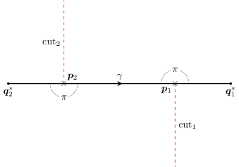
Figure 4.1. The geodesic $\gamma$ passing through two cone points, with a geometric diffraction in both cases

Using this local isometry we can define, for $(\bm{q}_{1},\bm{q}_{2})$ near $(\bm{q}_{1}^{*},\bm{q}_{2}^{*}),$ the functions $|\bm{q}_{i}-\bm{p}_{i}|$ and $|\bm{q}_{1}-\bm{q}_{2}|$ to be the Euclidean distance in $\mathbb{R}^{2}$ of the corresponding preimages.

For $t$ close to $t^{*}$ we can then define the following Lagrangian submanifold in $T^{*}\big{(}X^{\circ}\times X^{\circ}\big{)}$

$$\Lambda^{0} \,\stackrel{{\scriptstyle\textup{def}}}{{=}}\,N^{*}\big{\{}|\bm{q}_{2}-\bm{p}_{2}|+b+|\bm{p}_{1}-\bm{q}_{1}|=t\,\big{\}},$$

$$\Lambda^{1} \,\stackrel{{\scriptstyle\textup{def}}}{{=}}\,N^{*}\big{\{}|\bm{q}_{2}-\bm{p}_{1}|\,+|\bm{p}_{1}-\bm{q}_{1}|=t\,\big{\}},$$

$$\Lambda^{2} \,\stackrel{{\scriptstyle\textup{def}}}{{=}}\,N^{*}\big{\{}|\bm{q}_{2}-\bm{p}_{2}|\,+|\bm{p}_{2}-\bm{q}_{1}|=t\,\big{\}},$$

$$\Lambda^{3} \,\stackrel{{\scriptstyle\textup{def}}}{{=}}\,N^{*}\big{\{}|\bm{q}_{2}-\bm{q}_{1}|=t\,\big{\}},$$

It is straightforward to check that $\Lambda^{3}$ corresponds to direct propagation, $\Lambda^{1}$ corresponds to one diffraction at $\bm{p}_{1}$, $\Lambda^{2}$ to one diffraction at $\bm{p}_{2}$ and $\Lambda^{0}$ to two diffractions in a row at $\bm{p}_{2}$ and $\bm{p}_{1}.$

The aim of this section is the following

Proposition 4.1.

For $t>0$ fixed near $t^{*}$, the Schwartz kernel of $A_{1}\,\mathcal{U}(t)\,A_{2}$ is an intersecting Lagrangian distribution of order $0$ associated to the four Lagrangian submanifolds $(\Lambda_{0},\Lambda_{1},\Lambda_{2},\Lambda_{3})$.

Proof.

We begin with a decomposition of $A_{1}\,\mathcal{U}(t)\,A_{2}$ in which only one conic point plays a role in each factor. This is straightforward: we choose a time $t_{0}\in(a,a+b)$, say $t_{0}=a+\frac{b}{2}$, and we write $A_{1}\,\mathcal{U}(t)\,A_{2}=\left(A_{1}\,\mathcal{U}(t-t_{0})\right)\left(\mathcal{U}(t_{0})\,A_{2}\right)$. In terms of their Schwartz kernels, this is

(4.1) $$\mathcal{K}\!\left[A_{1}\,\mathcal{U}(t)\,A_{2}\right]\!(\bm{q}_{1},\bm{q}_{2})=\int_{X}\mathcal{K}\!\left[A_{1}\,\mathcal{U}(t-t_{0})\right](\bm{q}_{1},\bm{q})\cdot\mathcal{K}\!\left[\mathcal{U}(t_{0})\,A_{2}\right]\!(\bm{q},\bm{q}_{2})\,d\bm{q}.$$

Due to the assumptions on the microlocalizers $A_{i}$, the only points $\bm{q}$ that contribute to the singularities of (4.1) are points near $(b/2,0)$ in our coordinate system. In each factor of the composition above, the singularities of the half-wave kernel only meet one cone point. Thus, modulo smooth errors, we may replace the half-wave kernel by the half-wave kernel on an exact cone in each factor, allowing us to use the results of Section 2.

More precisely, in (4.1), to obtain a singularity $(\bm{q}_{1},\bm{\xi}_{1};\bm{q}_{2},\bm{\xi}_{2})$ in the canonical relation of $A_{1}\,\mathcal{U}(t)\,A_{2}$, we must have $(\bm{q},\bm{\xi};\bm{q}_{2},\bm{\xi}_{2})$ in the canonical relation of $\mathcal{U}(t_{0})\,A_{2}$ and $(\bm{q}_{1},\bm{\xi}_{1};\bm{q},\bm{\xi})$ in the canonical relation of $A_{1}\,\mathcal{U}(t-t_{0})$. For $t$ sufficiently close to $t^{*}$, this implies that $\bm{q}$ is close to the point $(b/2,0)$. That is, up to a $\mathcal{C}^{\infty}$ error, we may insert a cutoff function $\chi^{2}(\bm{q})$ into (4.1), where $\chi$ is supported close to $(0,b/2)$:

(4.2) $$\mathcal{K}\!\left[A_{1}\,\mathcal{U}(t)\,A_{2}\right]\!(\bm{q}_{1},\bm{q}_{2})\equiv\int_{X}\mathcal{K}\!\left[A_{1}\,\mathcal{U}(t-t_{0})\right](\bm{q}_{1},\bm{q})\cdot\chi^{2}(\bm{q})\cdot\mathcal{K}\!\left[\mathcal{U}(t_{0})\,A_{1}\right]\!(\bm{q},\bm{q}_{2})\,d\bm{q}$$

modulo $\mathcal{C}^{\infty}$ errors. Moreover, restricting the microlocal supports of $A_{1}$ and $A_{2}$ if needed, we may assume that the support of $\chi$ is contained in a ball that is isometric to the corresponding ball in $\mathbb{R}^{2}.$ By the above assumptions on the geodesic $\gamma$, the half-wave operators $\mathcal{U}(t_{0})$ and $\mathcal{U}(t-t_{0})$ in the compositions $\chi(\bm{q})\,\mathcal{U}(t_{0})\,A_{2}$ and $A_{1}\,\mathcal{U}(t-t_{0})\,\chi(\bm{q})$ can be replaced (up to a smooth error) by the corresponding wave kernels on the exact cones with cone points $\bm{p}_{1}$, resp.  $\bm{p}_{2}$, which we know from Section 2 are intersecting Lagrangian distributions associated to the diffractive and main fronts. That is, we can express the Schwartz kernel of $\chi(\bm{q})\,\mathcal{U}(t_{0})\,A_{2}$ in the oscillatory integral form

(4.3) $$(2\pi)^{-2}\int_{0}^{\infty}\int_{0}^{\infty}e^{i\phi_{2}(\bm{q},\bm{q}_{2},t_{0},s_{2},\omega_{2})}a_{2}(\bm{q},\bm{q}_{2},t_{0},s_{2},\omega_{2})\,d\omega_{2}\,ds_{2}$$

where $\phi_{2}$ is the phase function

(4.4) $$\phi_{2}\stackrel{{\scriptstyle\textup{def}}}{{=}}\big{[}|\bm{q}-\bm{p}_{2}(s_{2})|+|\bm{p}_{2}(s_{2})-\bm{q}_{2}|-t_{0}\big{]}\cdot\omega_{2},$$

where $\bm{p}_{2}(s_{2})$ has coordinates $(0,-\epsilon_{2}s_{2})$ and $|\cdot|$ denotes the Euclidean distance in $\mathbb{R}^{2}.$

Similarly, the Schwartz kernel of $A_{1}\,\mathcal{U}(t-t_{0})\,\chi(\bm{q})$ has the oscillatory integral representation

(4.5) $$(2\pi)^{-2}\int_{0}^{\infty}\int_{0}^{\infty}e^{i\phi_{1}(\bm{q}_{1},\bm{q},t-t_{0},s_{1},\omega_{1})}a_{1}(\bm{q}_{1},\bm{q},t-t_{0},s_{1},\omega_{1})\,d\omega_{1}\,ds_{1}$$

where $\phi_{1}$ is the phase function

(4.6) $$\phi_{1}\stackrel{{\scriptstyle\textup{def}}}{{=}}\big{[}|\bm{q}_{1}-\bm{p}_{1}(s_{1})|+|\bm{p}_{1}(s_{1})-\bm{q}|-(t-t_{0})\big{]}\cdot\omega_{1},$$

where now $\bm{p}_{1}(s_{1})$ has coordinates $(b,-\epsilon_{1}s_{1}).$ Here, $a_{i}$ is smooth, supported in $\omega_{i}\geqslant 1$, and is a symbol of order $1$ in $\omega_{i}$.

Therefore, (4.2) is given by an oscillatory integral (up to smooth errors) of the form

(4.7) $$(2\pi)^{-4}\int_{X_{\bm{q}}}\int_{\mathbb{R}^{2}_{\bm{\omega}}}\int_{s_{1}=0}^{\infty}\int_{s_{2}=0}^{\infty}e^{i\phi_{1}+i\phi_{2}}\,a_{1}(\bm{q}_{1},\bm{q},t-t_{0},s_{1},\omega_{1})\\ \times a_{2}(\bm{q},\bm{q}_{2},t_{0},s_{2},\omega_{2})\,ds_{1}\,ds_{2}\,d\omega_{1}\,d\omega_{2}\,d\bm{q}$$

We now show that in the overall phase function $\Phi\stackrel{{\scriptstyle\textup{def}}}{{=}}\phi_{1}+\phi_{2}$ we can eliminate the variables $(\bm{q},\omega_{2})$. This is possible if the following non-degeneracy condition is satisfied:

(4.8) $$d_{(\bm{q},\omega_{2})}\Phi=0\implies\det d^{2}_{(\bm{q},\omega_{2}),(\bm{q},\omega_{2})}\Phi\neq 0.$$

The condition $d_{\bm{q}}\Phi=0$ implies that $\bm{q}$ is on the segment $[p_{2}(s_{2}),p_{1}(s_{1})]$ and that $\omega_{1}=\omega_{2}$. The condition $d_{\omega_{2}}\Phi=0$ implies that $\bm{q}$ is at distance $t_{0}-|\bm{p}_{2}(s_{2})-\bm{q}_{2}|$ from $\bm{p}_{2}(s_{2}).$ Since the non-degeneracy condition is coordinate free and has to be verified with fixed $s_{1},s_{2},\omega_{1},\bm{q}_{1},\bm{q}_{2}$ we can choose for $\bm{q}$ cartesian coordinates $(x,y)$ in a rotated and translated coordinate frame, such that the origin corresponds to the critical point and the conical points $\bm{p}_{i}(s_{i})$ have the following coordinates: $\bm{p}_{1}(s_{1})=(B,0),~{}\bm{p}_{2}(s_{2})=(-A,0)$ with positive $A,~{}B.$ We observe that $A$ and $B$ depend on all remaining variables.

In these coordinates we have (we only keep $(x,y,\omega_{2})$ as variables since the other ones are fixed)

$$\Phi(x,y,\omega_{2})=\omega_{1}\cdot\left[|\bm{q}_{1}-\bm{p}_{1}(s_{1})|+\sqrt{(B-x)^{2}+y^{2}}-(t-t_{0})\right]\\ \mbox{}+\omega_{2}\cdot\left[\sqrt{(A+x)^{2}+y^{2}}+|\bm{q}_{2}-\bm{p}_{2}(s_{2})|-t_{0}\right]$$

We compute that

(4.9) $$d_{x}\Phi =\frac{(x-B)\omega_{1}}{\sqrt{(B-x)^{2}+y^{2}}}+\frac{(A+x)\omega_{2}}{\sqrt{(A+x)^{2}+y^{2}}},$$

$$d_{y}\Phi =\frac{y\omega_{1}}{\sqrt{(B-x)^{2}+y^{2}}}+\frac{y\omega_{2}}{\sqrt{(A+x)^{2}+y^{2}}},$$

$$d_{\omega_{2}}\Phi =\sqrt{(A+x)^{2}+y^{2}}+|\bm{q}_{2}-\bm{p}_{2}(s_{2})|-t_{0}$$

The critical point is easily seen to be $(x=0,y=0,\omega_{2}=\omega_{1}).$ We can then compute the Hessian of $\Phi$ in the $(x,y,\omega_{2})$-variables and evaluate it at the critical point:

(4.10) $$\begin{bmatrix}\partial_{xx}\Phi&0&1\\ 0&\omega_{1}C&0\\ 1&0&0\end{bmatrix},\quad C\stackrel{{\scriptstyle\textup{def}}}{{=}}\frac{1}{A}+\frac{1}{B}.$$

The determinant is $-C\omega_{1}<0$ so that the non-degeneracy condition is satisfied. It is straightforward to check that this matrix has two positive eigenvalues and one negative eigenvalue. The signature thus is $1.$

Hence, using the argument of Hörmander [HorFIO], we can write the oscillatory integral where we replace $(x,y,\omega_{2})$ by their values at the stationary point that we denote by $\bm{q}_{c}$. We obtain the oscillatory integral (writing $\omega$ for $\omega_{1}$)

(4.11) $$(2\pi)^{-5/2}\int_{-\infty}^{\infty}\int_{s_{1}=0}^{\infty}\int_{s_{2}=0}^{\infty}e^{i\Psi(t,\bm{q}_{1},\bm{q}_{2},s_{1},s_{2},\omega)}\tilde{a}(t,\bm{q}_{1},\bm{q}_{2},s_{1},s_{2},\omega)\,ds_{1}\,ds_{2}\,d\omega,$$

where the phase function $\Psi(t,\bm{q}_{1},\bm{q}_{2},s_{1},s_{2},\omega_{1})$ is seen to be

(4.12) $$\Psi \stackrel{{\scriptstyle\textup{def}}}{{=}}\big{[}|\bm{q}_{2}-\bm{p}_{2}(s_{2})|+|\bm{p}_{2}(s_{2})-\bm{q}_{c}|+|\bm{q}_{c}-\bm{p}_{1}(s_{1})|+|\bm{p}_{1}(s_{1})-\bm{q}_{1}|-t\big{]}\omega_{1}$$

$$=\big{[}|\bm{q}_{2}-\bm{p}_{2}(s_{2})|+|\bm{p}_{2}(s_{2})-\bm{p}_{1}(s_{1})|+|\bm{p}_{1}(s_{1})-\bm{q}_{1}|-t\big{]}\omega_{1},$$

and the amplitude is given by

(4.13) $$\tilde{a}(t,\bm{q}_{1},\bm{q}_{2},s_{1},s_{2},\omega)=e^{i\pi/4}(\omega C)^{-1/2}a_{1}(\bm{q}_{1},\bm{q}_{c},t-t_{0},s_{1},\omega)a_{2}(\bm{q}_{c},\bm{q}_{2},t_{0},s_{2},\omega).$$

We can now verify easily, using Definition 1.11 and Remark 1.13, that $\Psi$ parametrizes the given system of four Lagrangian submanifolds. Indeed, a simple computation shows that at $(t^{*},\bm{q}_{1}^{*},\bm{q}_{2}^{*},\omega^{*})=(c,(c-a,0),(-a,0),1)$ we have $d_{\omega,s_{1},s_{2}}\Psi(t,\bm{q}_{1}^{*},\bm{q}_{2}^{*},\omega^{*},0,0)=0$. Moreover, explicit computation shows that at this point the differential $d(\partial\Psi/\partial s_{1})$ is a nonzero multiple of $dy_{1}$, the differential $d(\partial\Psi/\partial s_{2})$ is a nonzero multiple of $dy_{2}$, and $d(\partial\Psi/\partial\omega_{1})$ has a nonzero $dt$ component. Thus these differentials are linearly independent, implying that the localized propagator is an intersecting Lagrangian distribution associated to the above system. It is not hard to check that the four Lagrangians correspond to no diffractions ($\Lambda_{3}$), one diffraction ($\Lambda_{1}$, $\Lambda_{2}$), arising from interaction with $\bm{p}_{1}$ or $\bm{p}_{2}$ respectively, and two diffractions ($\Lambda_{0}$). Finally, as $\tilde{a}$ in (4.13) is a symbol in $\omega$ of order $3/2$, we see directly from Proposition 1.12 that the order of the distribution (that is, the order on $\Lambda_{3}$, the direct front) is $0$ (where $t$ is treated as a parameter). ∎

To conclude this section, we compute the principal symbol of the wave kernel $\mathcal{U}(t)\stackrel{{\scriptstyle\textup{def}}}{{=}}e^{-it\sqrt{\Delta}}$ at the twice-diffracted Lagrangian $\Lambda_{0}$ using Proposition 1.14. This amounts to computing $\tilde{a}$, to leading order in $\omega$, at $s_{1}=s_{2}=0$. We will do the computation in the case $\epsilon_{1}=-1$ and $\epsilon_{2}=+1,$ as in Figure 4.1. The other cases are similar.

Clearly, from (4.13), we need the leading order behaviour of $a_{i}$ at $s_{i}=0$. This is given by (3.6). Substituting into (4.13), we find that when $s_{1}=s_{2}=0$,

(4.14) $$\tilde{a}(t,\bm{q}_{1},\bm{q}_{2},0,0,\omega)=e^{i\pi/4}C^{-1/2}(2\pi)^{2}S_{\alpha_{1}}(-\pi-\theta_{1})\sin\theta_{1}\big{(}|\bm{q}_{1}-\bm{p}_{1}|\,|\bm{q}_{c}-\bm{p}_{1}|\big{)}^{-1/2}\\ \times S_{\alpha_{2}}(\theta_{2})\sin\theta_{2}\big{(}|\bm{q}_{2}-\bm{p}_{2}|\,|\bm{q}_{c}-\bm{p}_{2}|\big{)}^{-1/2}\omega^{3/2}\text{ mod }S^{1/2}.$$

When $s_{1}=s_{2}=0$ we have

$$C=\frac{A+B}{AB}=\frac{|\bm{q}_{c}-\bm{p}_{1}|+|\bm{q}_{c}-\bm{p}_{2}|}{|\bm{q}_{c}-\bm{p}_{1}|\,|\bm{q}_{c}-\bm{p}_{2}|}=\frac{b}{|\bm{q}_{c}-\bm{p}_{1}|\,|\bm{q}_{c}-\bm{p}_{2}|}.$$

Using coordinates where $(r_{i},\theta_{i})$ are polar coordinates for $\bm{q}_{i}$ centered at $\bm{p}_{i}$, we can simplify (4.14) to

(4.15) $$\tilde{a}(t,\bm{q}_{1},\bm{q}_{2},0,0,\omega)=e^{i\pi/4}(2\pi)^{2}S_{\alpha_{1}}(-\pi-\theta_{1})S_{\alpha_{2}}(\theta_{2})\sin\theta_{1}\sin\theta_{2}\\ \times\Big{(}\frac{r_{1}r_{2}}{b}\Big{)}^{-1/2}\omega^{3/2}\text{ mod }S^{1/2}.$$

Using Proposition 1.14, and the identities

$$\Psi_{s_{1}}=\frac{\omega\,y_{2}}{|\bm{y}|}=\omega\sin(\theta_{1})\quad\text{and}\quad\Psi_{s_{2}}=\frac{\omega x_{2}}{|\bm{x}|}=\omega\sin(\theta_{2})$$

valid when $s_{1}=s_{2}=0$, we find that the principal symbol at the twice-diffracted Lagrangian $\Lambda_{0}$ is

(4.16) $$\left.\frac{1}{2\pi}\left[\frac{\tilde{a}(\bm{x},\bm{y},t_{0},t,0,0,\omega)}{\Psi_{s_{1}}\Psi_{s_{2}}}\right]\right|_{C_{0}}\left|\frac{\partial(r_{1},\theta_{1},\theta_{2},\omega,r_{1}+b+r_{2}-t)}{\partial(x,y,\omega)}\right|^{-\frac{1}{2}}|dr_{1}d\theta_{1}d\theta_{2}d\omega|^{\frac{1}{2}}\\ =\frac{2\pi\,e^{i\pi/4}}{\omega^{\frac{1}{2}}b^{\frac{1}{2}}}S_{\alpha_{2}}(\theta_{2})\,S_{\alpha_{1}}(-\pi-\theta_{1})\,|dr_{1}d\theta_{1}d\theta_{2}d\omega|^{\frac{1}{2}}.$$

5. Contributions to the wave trace of an isolated orbit with two geometric diffractions

As a byproduct of our approach we can compute in a rather straightforward way the leading contribution to the wave trace of any kind of periodic orbit, thus generalizing [Hil]. We present here the case of an isolated periodic geodesic that has two geometric diffractions (and no other diffractions).

More precisely, we assume that the orbit $\gamma$ diffracts at $\bm{p}_{1}$ and $\bm{p}_{2}$ (not necessarily distinct) and that the angles of diffraction are $-\pi$ and $+\pi.$ We construct as before the rectangle with cuts that is associated with this periodic geodesic. We see that near $\bm{p}_{1}$ the geodesic is locally the limit of non-diffractives geodesics that pass above $\bm{p}_{1}.$ Near $\bm{p}_{2}$ it is locally the limit of non-diffractive geodesics that pass below. It follows that one cannot translate the orbit to a nearby periodic orbit, so that the orbit is isolated as a periodic orbit.

Remark 5.1.

If instead of translating the orbit we rotate it then we do obtain non-diffractive geodesics that converge to $\gamma$ on any interval $[0,T]$ but these won’t be periodic.

Let $\bm{q}$ be a point on $\gamma,$ we intend to compute

$$\sigma_{\rho}(t)\stackrel{{\scriptstyle\textup{def}}}{{=}}\operatorname{Tr}(A_{1}\mathcal{U}(t)A_{2}\rho),$$

for $t$ close to the period $L$, $A_{i}$ is a microlocal projector near $(\bm{q},\xi^{*})$ and $\rho$ a bump function near $\bm{q}$ such that on the support of $\rho$ the principal symbols of $A_{1}$ and $A_{2}$ are identically $1$ on the lift of the geodesic. More precisely, we first choose $A_{1}$ and $A_{2}$ such that for $t$ close to $L,$ any geodesic of length $t$ whose starting point is in the microsupport of $A_{2}$ and whose endpoint is in the microsupport of $A_{1}$ stays close to $\gamma.$ The bump function is chosen afterwards.

We construct the Euclidean system of coordinates as before: the periodic orbit lies along the $x$-axis, with cone points $\bm{p}_{2}$ located at $(0,0)$ and $\bm{p}_{1}$ at $(b,0)$, and we identify $(x,y)$ with $(x+L,y)$, where $L$ is the period.

According to Section 4, the Schwartz kernel of the half-wave operator $A_{1}\mathcal{U}(t)A_{2}$ after two diffractions has the following oscillatory integral representation

(5.1) $$(2\pi)^{-5/2}\int_{0}^{\infty}\int_{0}^{\infty}\int_{0}^{\infty}e^{i\psi(\bm{x},\bm{y},t,s_{1},s_{2},\omega)}\,\tilde{a}(t,\bm{q}_{1},\bm{q}_{2},s_{1},s_{2},\omega)\,ds_{1}\,ds_{2}\,d\omega,$$

where $\psi$ is given by

$$\psi(t,\bm{q}_{1},\bm{q}_{2},s_{1},s_{2},\omega)=\big{[}|\bm{q}_{2}-\bm{p}_{2}(s_{2})|+|\bm{p}_{2}(s_{2})-\bm{p}_{1}(s_{1})|+|\bm{p}_{1}(s_{1})-\bm{q}_{1}|-t\big{]}\cdot\omega$$

and $\tilde{a}$ is given by (4.15):

$$\tilde{a}(t,\bm{q}_{1},\bm{q}_{2},0,0,\omega)\sim(2\pi)^{2}\cdot e^{i\frac{\pi}{4}}\cdot\frac{\sin\theta_{1}\cdot S_{\alpha_{1}}(-\pi-\theta_{1})\cdot\sin\theta_{2}\cdot S_{\alpha_{2}}(\theta_{2})}{(r_{1}br_{2})^{\frac{1}{2}}}\cdot\omega^{\frac{3}{2}}.$$

We are thus lead to compute

(5.2) $$\sigma_{\rho}(t)\stackrel{{\scriptstyle\textup{def}}}{{=}}(2\pi)^{-5/2}\int_{X}\int_{0}^{\infty}\int_{0}^{\infty}\int_{0}^{\infty}e^{i\psi(t,\bm{q}+(L,0),\bm{q},s_{1},s_{2},\omega)}\tilde{a}\,\rho(\bm{q})\,ds_{1}ds_{2}d\bm{q}d\omega,$$

where we have set $\bm{q}_{2}=\bm{q}$ and $\bm{q}_{1}=\bm{q}+(L,0)$.

We choose to parametrize $\bm{q}$ by $(x,y)$: the Euclidean coordinates near $\bm{q}_{2}^{*}.$ In this oscillatory integral, we first perform a stationary phase with respect to $y.$ We denote by $y_{c}$ the stationary (critical) point. We observe geometrically that $(x,y_{c})$ is on the segment $[\bm{p}_{1}(s_{1}),\bm{p}_{2}(s_{2})].$ Moreover, we compute

$$|\partial^{2}_{y}\psi(t,(x,y_{c}),0,0,\omega)|=\frac{|L-b|}{|x||L-b-x|}\cdot\omega.$$

It follows that the critical point remains non-degenerate for small $(s_{1},s_{2}).$ Since geometrically, it is obvious that the critical point is a minimum, it also follows that the signature is $+1.$

We now observe that the phase, when evaluated at the critical point becomes independent of the remaining $x.$ More precisely it is given by $\tilde{\psi}$ where we have set

(5.3) $$\tilde{\psi}(t,s_{1},s_{2},\omega)=\Big{[}\sqrt{b^{2}+(s_{1}+s_{2})^{2}}+\sqrt{(L-b)^{2}+(s_{1}+s_{2})^{2}}-t\Big{]}\cdot\omega.$$

We thus obtain after applying the stationary phase:

$$\sigma_{\rho}(t)=\int_{0}^{L}\int_{0}^{\infty}\int_{0}^{\infty}\int_{0}^{\infty}e^{i\tilde{\psi}}A(t,x,s_{1},s_{2},\omega)\rho((x,y_{c}))\,ds_{1}\,ds_{2}\,d\omega\,dx,$$

where $A$ is a symbol that, at leading order and for $s_{1}=s_{2}=0$, reads

$$A(t,x,0,0,\omega) \sim(2\pi)^{1/2-5/2}e^{i\frac{\pi}{4}}\tilde{a}(t,(x+L,y_{c}),(x,y_{c}),0,0,\omega)$$

$$\hskip 72.26999pt\mbox{}\times|\partial^{2}_{y}\psi(t,(x,y_{c}),0,0,\omega)|^{-\frac{1}{2}}\rho(x,y_{c})$$

$$\sim i\cdot\frac{\sin(\theta_{1})\cdot S_{\alpha_{1}}(-\pi-\theta_{1})\cdot\sin(\theta_{2})\cdot S_{\alpha_{2}}(\theta_{2})}{\sqrt{b\cdot|x||L-b-x|}}\cdot\frac{\sqrt{|x||L-b-x|}}{\sqrt{L-b}}\cdot\omega$$

$$\sim i\cdot\frac{\sin\theta_{1}\cdot S_{\alpha_{1}}(-\pi-\theta_{1})\cdot\sin\theta_{2}\cdot S_{\alpha_{2}}(\theta_{2})}{\sqrt{b(L-b)}}\cdot\omega.$$

It remains to evaluate an oscillatory integral of the form

$$I(t)\stackrel{{\scriptstyle\textup{def}}}{{=}}\int_{0}^{L}\int_{0}^{\infty}\int_{0}^{\infty}\int_{0}^{\infty}e^{i\tilde{\psi}(t,s_{1},s_{2},\omega)}\tilde{A}(t,x,s_{1},s_{2},\omega)\cdot\omega\,ds_{1}\,ds_{2}\,d\omega\,dx$$

in which $\tilde{A}$ is a symbol in $\omega$.

If we forget the restriction on the domain for $(s_{1},s_{2})$, this is a standard oscillatory integral and the phase has a smooth submanifold of fixed point. The restriction on the domain makes it a little less standard. Although we could perform a general treatment for this kind of oscillatory integrals, in our case, the nature of the phase allows for a more direct computation.

We first make the change of variables $u=s_{1}+s_{2},~{}v=s_{1}-s_{2}.$ In these coordinates, $\tilde{\psi}$ is independent of $v$; we write $\tilde{\psi}(t,u,\omega)$ for the phase expressed in these coordinates. Notice that, by (5.3), it is a smooth function of $u^{2}$, and is stationary in $u$ only at $u=0$. The domain of integration becomes $u\geq 0$ and $-u\leqslant v\leqslant u.$ We obtain the integral

$$I(t)=\int_{0}^{\infty}\int_{0}^{\infty}e^{i\tilde{\psi}(t,u,\omega)}\left[\frac{1}{2}\int_{-u}^{u}\tilde{A}(u,v,\omega)dv\right]du\,d\omega.$$

Since the factor in square brackets vanishes at $u=0$, the leading contribution of this integral is obtained by performing an integration by parts in $u$. To do this we write

$$\tilde{\psi}(t,u,\omega)=(t-L)\omega+\tilde{\tilde{\psi}}(t,u,\omega),\quad\tilde{\tilde{\psi}}(t,u,\omega)=O(u^{2}),\ u\to 0.$$

Then we have $\lim_{u\rightarrow 0}\frac{\partial_{u}\tilde{\tilde{\psi}}(u,\omega)}{u}=\partial^{2}\tilde{\psi}(0,\omega)\neq 0.$ We obtain

$$I(t)\sim i\int_{0}^{\infty}e^{i(t-L)\omega}\tilde{A}_{0}(0,0,\omega)(\partial_{u}^{2}\tilde{\psi}(0,\omega))^{-1}d\omega$$

where the index $0$ means that we have taken the principal part of $\tilde{A}.$

It remains to evaluate all the quantities in our case observing that when $s_{1},s_{2}$ go to $0,$ $\theta_{1}$ go to $0$ and $\theta_{2}$ go to $\pi.$ Using (B.11) and (5.3), we have

$$\lim_{\theta_{1}\rightarrow 0}\sin\theta_{1}S_{\alpha_{1}}(-\pi-\theta_{1}) =\,\frac{1}{2\pi}$$

$$\lim_{\theta_{2}\rightarrow\pi}\sin\theta_{2}S_{\alpha_{2}}(\theta_{2}) =\,-\frac{1}{2\pi}$$

$$\partial^{2}_{u}\tilde{\psi}(0,\omega) =\omega\cdot\frac{L}{b(L-b)}.$$

Putting everything together we obtain:

$$\sigma_{\rho}(t) \,\sim\int_{0}^{\infty}e^{i\omega(L-t)}\frac{\sqrt{b(L-b)}}{4\pi^{2}L}d\omega\cdot\int_{0}^{L}\rho(x,0)dx$$

$$\,\sim\frac{1}{i}\frac{\sqrt{b(L-b)}}{4\pi^{2}L}\cdot(t-L-i0)^{-1}\cdot\int_{0}^{L}\rho(x,0)dx$$

The contribution of the whole periodic orbit is obtained by using a covering argument (i.e. choosing carefully near each point $A_{1},A_{2}$ and $\rho$ so that in the end $\sum\rho$ is identically $1$ in a neighbourhood of the geodesic). In the process, we have to be careful near the cone point. The contribution of a (small) neighbourhood of the cone point can be computed using the following trick (that is already used in [Hil] and [Wun]).

Suppose $\rho_{c}$ is a function that is identically $1$ near $\bm{p}_{1}.$ We want to compute

$$\sigma_{\rho_{C}}(t)\,\stackrel{{\scriptstyle\textup{def}}}{{=}}\,\operatorname{Tr}(\mathcal{U}(t)\rho_{c})$$

We insert microlocal cutoffs so that, up to a smooth remainder we have

$$\sigma_{\rho_{C}}(t)=\operatorname{Tr}(A_{1}\mathcal{U}(t-t_{0})A_{2}U(t_{0})\rho_{c}).$$

Using the cyclicity of the trace we need to calculate

$$\sigma_{\rho_{C}}(t)=\operatorname{Tr}(U(t_{0})\rho_{c}A_{1}\mathcal{U}(t-t_{0})A_{2}).$$

In the latter expression, thanks to the cutoffs, all the operations (composition and taking the trace) take place away of the conical point. So we can proceed as before.

In the end, if we sum all the contributions, it will amount to sum all the contributions $\int\rho(x,0)dx$ and this will give the length of the geodesic.

We obtain the following proposition.

Proposition 5.2.

On a ESCS, the leading contribution to the wave trace of an isolated periodic diffractive orbit with two geometric diffraction is

$$\frac{1}{4i\pi^{2}}\cdot\sqrt{b(L-b)}\cdot(t-L-i0)^{-1}.$$

Remark 5.3.

As a point of comparison, we recall the analogous leading-order contribution of a nondegenerate closed orbit $\gamma$ on a compact, smooth manifold in the trace theorem of Duistermaat and Guillemin [DuiGui]:

$$(2\pi)^{-1}L\,i^{\sigma_{\gamma}}\,\big{|}\mathrm{Id}-P_{\gamma}\big{|}^{-\frac{1}{2}}(t-L-i0)^{-1}.$$

Here, $P_{\gamma}$ is the Poincaré return map in the directions transverse to the level set of the symbol and to the flow direction, and $i^{\sigma_{\gamma}}$ is a Maslov factor (with $\sigma_{\gamma}$ the Morse index of the geodesic). The singularity we obtain here from an isolated periodic orbit with two geometric diffractions is thus of the same order.

We can also compare this with the singularity contributed by a non-geometric diffractive periodic orbit with one diffraction, as computed in [Hil, Theorem 2]. This has leading singularity $(t-L-i0)^{-1/2}$ and is hence one half order more regular. On the other hand, the singularity contributed by a cylinder of periodic geodesics is to leading order $(t-L-i0)^{-3/2}$, from op. cit. which is half an order more singular.

Notice that a cylinder of periodic geodesics necessarily has geometrically diffracted geodesics at its boundary. In the second article in this series, we intend to use the analysis of the present paper to compute higher order terms in the wave trace singularity arising from such a cylinder.

Appendix A Domains of operators and admissible asymptotics at the cone point

In the course of our construction of the wave propagators on $C_{4\pi}$, we needed information about the domains of operators related to the Laplace-Beltrami operator $\Delta_{g}$. The first such result was a description of the domain of the adjoint operator $\overline{\Delta_{g}}{}^{*}$.

Lemma A.1.

Let $\rho\in\mathcal{C}^{\infty}((0,\infty)_{r})$ be a smooth cutoff satisfying $\rho\equiv 1$ for $r\leqslant 1$ and $\rho\equiv 0$ for $r\geqslant 2$. Then the domain of $\left(\overline{\Delta_{g}}\right)^{*}$ as an unbounded operator on $L^{2}(C_{4\pi})$ is

(A.1) $$\overline{\mathfrak{D}}{}^{*}=\overline{\mathfrak{D}}\oplus\mathrm{Span}_{\mathbb{C}}\!\left\{\rho,\rho\log(r),\rho\,r^{\frac{1}{2}}\exp\!\left[\pm\frac{i\theta}{2}\right],\rho\,r^{-\frac{1}{2}}\exp\!\left[\pm\frac{i\theta}{2}\right]\right\}.$$

Proof.

Using the symmetry of $\Delta_{g}$, we may decompose $\overline{\mathfrak{D}}{}^{*}$ as

$$\overline{\mathfrak{D}}{}^{*}=\overline{\mathfrak{D}}\oplus\operatorname{Null}(\Delta_{g}-\alpha_{1})\oplus\operatorname{Null}(\Delta_{g}-\alpha_{2})$$

for any distinct $\alpha_{1}$ and $\alpha_{2}$ lying outside the spectrum of $\Delta_{g}$ (cf. [ReeSim2]). Moreover, nonnegativity of $\Delta_{g}$ implies that it is sufficient to let $\alpha_{j}=-\beta_{j}^{2}$ for distinct choices of $\beta_{j}$. Thus, let us suppose that $u$ is an element of $\operatorname{Null}(\Delta_{g}+\beta^{2})$, i.e.,

(A.2) $$\left(\Delta_{g}+\beta^{2}\right)u(r,\theta)=-\frac{1}{r^{2}}\left[r^{2}\partial_{r}^{2}+r\partial_{r}-\left(\beta^{2}r^{2}-\partial_{\theta}^{2}\right)\right]u(r,\theta)=0.$$

By separating variables using the spectral projectors (2.14), we may rewrite $u$ as a Fourier series of the form

$$u(r,\theta)=\frac{1}{\sqrt{4\pi}}\sum_{j\in\mathbb{Z}}\hat{u}_{j}(r)\exp\!\left[i\,\frac{j}{2}\,\theta\right].$$

Then the quality (A.2) implies the corresponding equality

(A.3) $$\left(L_{j}+\beta^{2}\right)\hat{u}_{j}(r)\stackrel{{\scriptstyle\textup{def}}}{{=}}-\frac{1}{r^{2}}\left[r^{2}\partial_{r}^{2}+r\partial_{r}-\left(\beta^{2}r^{2}+\frac{j^{2}}{4}\right)\right]\hat{u}_{j}(r)=0.$$

Introducing the change of variables $s=\beta r$ into (A.3), this differential equation becomes

(A.4) $$-\frac{\beta^{2}}{s^{2}}\left[s^{2}\partial_{s}^{2}+s\partial_{s}-\left(s^{2}+\frac{j^{2}}{4}\right)\right]\hat{u}_{j}(\beta^{-1}s)=0,$$

which is the modified Bessel equation, up to the overall factor of $-\frac{\beta^{2}}{s^{2}}$. Thus, the Fourier coefficients $\hat{u}_{j}$ must be linear combinations of the modified bessel functions $I_{\frac{j}{2}}(s)$ and $K_{\frac{j}{2}}(s)$.

Now, observe that the condition that our original function $u$ is an element of $L^{2}(C_{4\pi})$ forces each of the Fourier coefficients $\hat{u}_{j}(\beta^{-1}s)$ to be elements of the function space $L^{2}((0,\infty)_{s},sds)$. Indeed, the Fourier decomposition in $\theta$ induces a factoring

$$L^{2}(C_{4\pi})=\ell^{2}\!\left(\mathbb{Z};L^{2}((0,\infty)_{r},rdr)\right),$$

and our change of variables identifies $L^{2}((0,\infty)_{r},rdr)$ with $L^{2}((0,\infty)_{s},sds)$. This implies that the only admissible solutions to (A.4) are

$$\hat{u}_{0}(\beta^{-1}s)=K_{0}(s),\quad\hat{u}_{\pm 1}(\beta^{-1}s)=K_{\frac{1}{2}}(s),\quad\text{and}\quad\hat{u}_{j}(\beta^{-1}s)=0\text{ for $|j|\geqslant 2$}.$$

These are the only modified Bessel functions which are globally in $L^{2}((0,\infty)_{s},sds)$, as may be easily gleaned from their asymptotics as $s\to 0$ and $s\to\infty$ in [AbrSte]. Hence,

(A.5) $$\operatorname{Null}(\Delta_{g}+\beta^{2})=\mathrm{Span}_{\mathbb{C}}\!\left\{K_{0}(\beta r),K_{\frac{1}{2}}(\beta r)\exp\!\left[\frac{i\theta}{2}\right],K_{\frac{1}{2}}(\beta r)\exp\!\left[-\frac{i\theta}{2}\right]\right\}.$$

Let $\rho\in\mathcal{C}^{\infty}((0,\infty)_{r})$ be a cutoff as in the statement of the lemma, and observe that

$$\left[1-\rho(r)\right]K_{0}(\beta r)\quad\text{and}\quad\left[1-\rho(r)\right]K_{\frac{1}{2}}(\beta r)$$

are both Schwartz in $r$ and vanish at the cone point. This shows they are elements of $\overline{\mathfrak{D}}$, which in turn implies that $\overline{\mathfrak{D}}{}^{*}$ is equal to

$$\overline{\mathfrak{D}}\oplus\mathrm{Span}_{\mathbb{C}}\left\{\rho\,K_{0}(\beta_{1}r),\rho\,K_{\frac{1}{2}}(\beta_{1}r)\exp\!\left[\pm\frac{i\theta}{2}\right],\rho\,K_{0}(\beta_{2}r),\rho\,K_{\frac{1}{2}}(\beta_{2}r)\exp\!\left[\pm\frac{i\theta}{2}\right]\right\}$$

for any two distinct choices of $\beta_{j}>0$. Similarly, since

$$K_{0}(x)=-\log\!\left(\frac{x}{2}\right)-\gamma+\mathrm{O}(x)\text{ as $x\to 0$}\quad\text{and}\quad K_{\frac{1}{2}}(x)=\left(\frac{\pi}{2x}\right)^{\frac{1}{2}}e^{-x},$$

where $\gamma$ is the Euler-Mascheroni constant and $\Gamma(z)$ is the $\Gamma$-function, we have that

$$\mathrm{Span}_{\mathbb{C}}\left\{\rho\,K_{0}(\beta_{1}r),\rho\,K_{\frac{1}{2}}(\beta_{1}r)\exp\!\left[\pm\frac{i\theta}{2}\right],\rho\,K_{0}(\beta_{2}r),\rho\,K_{\frac{1}{2}}(\beta_{2}r)\exp\!\left[\pm\frac{i\theta}{2}\right]\right\}\\ \mbox{}\equiv\mathrm{Span}_{\mathbb{C}}\!\left\{\rho,\rho\log(r),\rho\,r^{\frac{1}{2}}\exp\!\left[\pm\frac{i\theta}{2}\right],\rho\,r^{-\frac{1}{2}}\exp\!\left[\pm\frac{i\theta}{2}\right]\right\}\,\left(\text{mod }\overline{\mathfrak{D}}\right).$$

This concludes the proof. ∎

The other piece of information about domains we needed was the expansion of elements of the Friedrichs domain $\mathcal{D}_{2}$ at the cone point given in Lemma 2.1. We now prove this lemma.

Proof of Lemma 2.1.

The Friedrichs domain $\mathcal{D}_{2}$ is characterized as the subspace of $\overline{\mathfrak{D}}{}^{*}$ which is included in the Dirichlet form domain associated to $\Delta_{g}$, i.e., those distributions $u$ which are bounded in

$$Q_{\Delta_{g}}(u)=\left<u,u\right>_{L^{2}}+\left<u,\Delta_{g}u\right>_{L^{2}}.$$

As the Dirichlet form domain is precisely $H^{1}(C_{4\pi})$, we may conclude from the description (A.1) of $\overline{\mathfrak{D}}{}^{*}$ that

$$\mathcal{D}_{2}=\overline{\mathfrak{D}}\oplus\mathrm{Span}_{\mathbb{C}}\!\left\{\rho,\rho\,r^{\frac{1}{2}}\exp\!\left[\frac{i\theta}{2}\right],\rho\,r^{\frac{1}{2}}\exp\!\left[-\frac{i\theta}{2}\right]\right\}$$

since these are the only elements of $\overline{\mathfrak{D}}{}^{*}\big{/}\overline{\mathfrak{D}}$ which are elements of $H^{1}(C_{4\pi})$. The lemma follows. ∎

Appendix B Geometric theory of diffraction

In this appendix we proceed with a construction of the kernel of the wave propagator that allows to compute explicitly the symbol on both Lagrangians $\Lambda^{\bm{\mathsf{G}}}$ and $\Lambda^{\bm{\mathsf{D}}}$ away of their intersection. For the diffracted part, this is known in the literature as the geometric theory of diffraction [Keller] and we provide an interpretation of this construction based on scattering of waves on the cone $C_{\alpha}$.

At the direct front, the symbol is just as it is on $\mathbb{R}^{2}$. Recall that, on $\mathbb{R}^{2}$, the half-wave kernel as a distributional half-density is

(B.1) $$(2\pi)^{-2}\int e^{i((x-y)\cdot\xi-t|\xi|)}\,d\xi\big{|}dxdy\big{|}^{\frac{1}{2}}.$$

Let $\mathbf{e}_{1}$ be a unit vector in the plane pointing from $x$ to $y$, and let $(\mathbf{e}_{1},\mathbf{e}_{2})$ be an oriented orthonormal basis. We write $\xi=\omega\mathbf{e}_{1}+\rho\mathbf{e}_{2}$. Then the integral can be written

(B.2) $$(2\pi)^{-2}\int e^{i(|x-y|\omega-t\sqrt{\omega^{2}+\rho^{2}})}\,d\rho\,d\omega\big{|}dxdy\big{|}^{\frac{1}{2}}.$$

Assume $t>0$. Then there are stationary points on the line $\left\{\rho=0,\omega>0\right\}$. We can integrate out $\rho$, and to leading order (that is, replacing the expression with the leading term in the stationary phase expansion at $\rho=0$) we get

(B.3) $$(2\pi)^{-\frac{3}{2}}\int e^{i(|x-y|-t)\omega}\chi(\omega)e^{-\frac{i\pi}{4}}\left(\frac{\omega}{t}\right)^{\frac{1}{2}}\,d\omega\big{|}dxdy\big{|}^{\frac{1}{2}}$$

where $\chi\in\mathcal{C}^{\infty}(\mathbb{R})$ is zero for $\omega<1$ and $1$ for $\omega\geq 2$. Thus, the principal symbol of this distribution at $N^{*}\{|x-y|=t\}$, for $t$ fixed, is

(B.4) $$e^{-\frac{i\pi}{4}}\chi(\omega)\left(\frac{\omega}{t}\right)^{\frac{1}{2}}\big{|}dydsd\omega\big{|}^{\frac{1}{2}}$$

for $s$ the arc length along the circle $\{|x-y|=t\}$ and $\omega$ the cotangent variable dual to $|x-y|-t$.

We now return to $C_{\alpha}$, the cone of angle $\alpha$, and we restrict our attention to $t>0$. On the diffracted front $\Lambda^{\bm{\mathsf{D}}}$ and away from the direct front, the half-wave kernel $\bm{U}(t)$ takes the oscillatory integral form

(B.5) $$(2\pi)^{-\frac{3}{2}}\int e^{i(r+r^{\prime}-t)\cdot\omega}\,K(r,\theta;r^{\prime},\theta^{\prime};\omega)\left|rdrd\theta\,r^{\prime}dr^{\prime}d\theta^{\prime}\right|^{\frac{1}{2}}.$$

The amplitude $K(r,\theta;r^{\prime},\theta^{\prime};\omega)$ is a symbol of order 0 in $\omega$, as follows from the kernel $\bm{U}(t)$ being of order $-\frac{1}{2}$ (for each fixed $t$) at $\Lambda^{\bm{\mathsf{D}}}$. We consider how this part of the propagator acts on a particular initial condition. Consider the exact solution to the half-wave equation given by

(B.6) $$\sqrt{\frac{\pi}{2}}\Big{(}\int e^{-i\lambda t^{*}}J_{|\nu|}(\lambda r)\tilde{\chi}(\lambda)\,d\lambda\Big{)}e^{i\nu\theta},$$

where $\tilde{\chi}\in\mathcal{C}^{\infty}(\mathbb{R})$ is supported in $[2,\infty)$ and identically $1$ for $\lambda\geq 4$, say, and where $\nu=\frac{2\pi\ell}{\alpha}$ for some integer $\ell$. This distribution (B.6) is conormal to $\{r=-t\}$ for $t<0$ and to $\{r=t\}$ for $t>0$, as can be seen by using the expansion for the Bessel function as its argument gets large:

(B.7) $$J_{|\nu|}(z)=\sqrt{\frac{2}{\pi z}}\cos\!\left(z-\frac{|\nu|\pi}{2}-\frac{\pi}{4}\right)\sum_{j=0}^{\infty}a_{j}(z)$$

where $a_{j}\in S^{-j}(\mathbb{R}_{z})$ are the homogeneous terms in the expansion in $z$ with $a_{0}(z)\equiv 1$. Therefore, up to a smooth error, the solution (B.6) has the form

$$e^{i\nu\theta}\int e^{-i\lambda t}\Big{(}e^{i(\lambda r-|\nu|\pi/2-\pi/4)}+e^{-i(\lambda r-\nu\pi/2-\pi/4)}\Big{)}a(\lambda r)(\lambda r)^{-\frac{1}{2}}\,d\lambda$$

for $a\in S^{0}(\mathbb{R})$. The singularities for $t<0$, say $t=-t_{*}$, take the form

(B.8) $$(2\pi)^{-\frac{1}{2}}e^{i\nu\theta}\int e^{-i(\lambda(r-t_{*})-|\nu|\pi/2-\pi/4)}a(\lambda r)(\lambda r)^{-\frac{1}{2}}\,d\lambda,$$

and for $t>0$, say $t=+t_{*}$,

(B.9) $$(2\pi)^{-\frac{1}{2}}e^{i\nu\theta}\int e^{i(\lambda(r-t_{*})-|\nu|\pi/2-\pi/4)}a(\lambda r)(\lambda r)^{-\frac{1}{2}}\,d\lambda.$$

On the other hand, if we apply the wave kernel $e^{-2it_{*}\sqrt{\Delta}}$ to the initial condition (B.8) we obtain (B.9) up to smooth terms. The direct front, away from the diffracted wave, does not contribute for $t>t_{*}$, and the singularities come purely from the diffracted front (except at the intersection, where $\theta-\theta^{\prime}\equiv\pm\pi\,\left(\text{mod }\alpha\right)$). Away from the direct front, applying (B.5) to (B.8) gives us

$$(2\pi)^{-\frac{3}{2}}\int e^{i(r+r^{\prime}-2t_{*})\omega}K(r,\theta;r^{\prime},\theta^{\prime};\omega)e^{i(-\lambda(r^{\prime}-t_{*})+|\nu|\pi/2+\pi/4)}(\lambda r^{\prime})^{-\frac{1}{2}}a(\lambda r^{\prime})e^{i\nu\theta^{\prime}}\\ \mbox{}\times r^{\prime}\,dr^{\prime}\,d\theta^{\prime}\,d\omega$$

and after applying stationary phase in the $(r^{\prime},\omega)$-variables we obtain

$$(2\pi)^{-\frac{1}{2}}\int e^{i(r-t_{*})\lambda}(\lambda r)^{-\frac{1}{2}}\chi(\lambda)\left\{e^{i|\nu|\pi/2}e^{i\pi/4}\int(rr^{\prime})^{\frac{1}{2}}K(r,\theta;r^{\prime},\theta^{\prime};\omega)e^{i\nu\theta^{\prime}}\,d\theta^{\prime}\right\}d\lambda.$$

This must yield (B.9) up to smooth terms. Therefore the leading-order part of the amplitude $S$, viewed as a Schwartz kernel in the $(\theta,\theta^{\prime})$-variables, maps $e^{i\nu\theta}$ to the quantity

$$(2\pi)^{\frac{1}{2}}e^{-i\pi/2}e^{-i|\nu|\pi}(rr^{\prime})^{-\frac{1}{2}}e^{i\nu\theta}.$$

Hence, the principal part of $K$ corresponds to the operator

$$-i(2\pi)^{\frac{1}{2}}(rr^{\prime})^{-\frac{1}{2}}e^{-i\pi\sqrt{\smash[b]{\Delta_{\mathbb{S}^{1}_{\alpha}}}}},$$

since $e^{i\nu\theta}$ is an eigenfunction of $\sqrt{\smash[b]{\Delta_{\mathbb{S}^{1}_{\alpha}}}}$ with eigenvalue $|\nu|$.

We can compare this principal part to the absolute scattering matrix $S(\lambda)$ for the cone $C_{\alpha}$. This is, by definition, the map from the “incoming boundary data” of generalized eigenfunctions of $\sqrt{\smash[b]{\Delta_{\mathbb{S}^{1}_{\alpha}}}}$ with eigenvalue $\lambda$, to the “outgoing boundary data”. These are the coefficients of $e^{-i\lambda r}$, respectively $e^{+i\lambda r}$, in the expansions of the generalized eigenfunction as $r\to\infty$. By inspection of the generalized eigenfunctions

$$J_{\nu}(\lambda r)e^{i\nu\theta},$$

and (B.7), we see that this operator is $-ie^{-i\pi\sqrt{\smash[b]{\Delta_{\mathbb{S}^{1}_{\alpha}}}}}$. Hence, we obtain at leading order and provided $\theta-\theta^{\prime}\not\equiv\pm\pi\,\left(\text{mod }\alpha\right)$

$$K(r,\theta,r^{\prime},\theta^{\prime})\sim(2\pi)^{\frac{1}{2}}(rr^{\prime})^{-\frac{1}{2}}S_{\alpha}(\theta-\theta^{\prime})$$

where $S_{\alpha}(\theta-\theta^{\prime})$ is the kernel of the absolute scattering matrix for the cone of angle $\alpha$ or, equivalently the kernel of $-ie^{-i\pi\Delta_{\mathbb{S}^{1}_{\alpha}}}$

The principal symbol of the diffracted wave is therefore the leading-order part of

$$K(r,\theta;r^{\prime},\theta^{\prime};\omega)|drd\theta d\theta^{\prime}d\omega|^{\frac{1}{2}}\left|\frac{\partial(r,\theta;r^{\prime},\theta^{\prime};\omega)}{\partial(x,y,\omega)}\right|^{-\frac{1}{2}}\\ \equiv-i\sqrt{2\pi}(rr^{\prime})^{-\frac{1}{2}}\mathcal{K}\!\left[e^{-i\pi\sqrt{\smash[b]{\Delta_{\mathbb{S}^{1}_{\alpha}}}}}\right](\theta,\theta^{\prime})\cdot(rr^{\prime})^{\frac{1}{2}}|drd\theta d\theta^{\prime}d\omega|^{\frac{1}{2}}\,\left(\text{mod }S^{-1}\right),$$

which after simplification is

(B.10) $$\sqrt{2\pi}\,S_{\alpha}(\theta-\theta^{\prime})|drd\theta d\theta^{\prime}d\omega|^{\frac{1}{2}}.$$

The distribution $S_{\alpha}$ can be computed using Fourier series. Indeed, since it is the kernel of $-ie^{-i\pi\Delta_{\mathbb{S}^{1}_{\alpha}}}$ we have

(B.11) $$S_{\alpha}(\theta) =\frac{-i}{\alpha}\sum_{k\in\mathbb{Z}}e^{-i\pi\big{|}\frac{2k\pi}{\alpha}\big{|}}e^{-\frac{2ik\pi}{\alpha}\theta}$$

$$=\frac{-i}{\alpha}\Big{[}1+\sum_{k\geq 1}e^{-\frac{2ik\pi}{\alpha}(\pi-\theta)}+\sum_{k\geq 1}e^{-\frac{2ik\pi}{\alpha}(\pi+\theta)}\Big{]}$$

$$=\frac{-i}{\alpha}\Big{[}1+\frac{e^{-\frac{2i\pi}{\alpha}(\pi-\theta)}}{1-e^{-\frac{2i\pi}{\alpha}(\pi-\theta)}}+\frac{e^{-\frac{2i\pi}{\alpha}(\pi+\theta)}}{1-e^{-\frac{2i\pi}{\alpha}(\pi+\theta)}}\Big{]}$$

$$=\frac{-i}{\alpha}\Big{[}1+\frac{e^{-\frac{i\pi}{\alpha}(\pi-\theta)}}{2i\sin\big{(}\frac{\pi}{\alpha}(\pi-\theta)\big{)}}+\frac{e^{-\frac{i\pi}{\alpha}(\pi+\theta)}}{2i\sin\big{(}\frac{\pi}{\alpha}(\pi+\theta)\big{)}}\Big{]}$$

$$=\frac{-1}{2\alpha}\frac{\sin(\frac{2\pi^{2}}{\alpha})}{\sin\big{(}\frac{\pi}{\alpha}(\pi-\theta)\big{)}\sin\big{(}\frac{\pi}{\alpha}(\pi+\theta)\big{)}}$$

In the case $\alpha=4\pi$, this simplifies to

(B.12) $$S_{4\pi}(\theta)=\frac{-1}{8\pi}\cdot\frac{1}{\sin(\frac{\pi-\theta}{4})\sin(\frac{\pi+\theta}{4})}=\frac{-1}{4\pi}\cdot\frac{1}{\cos\frac{\theta}{2}}.$$

Summarizing this computation we have the following proposition.

Proposition B.1.

Microlocally near the diffracted front $\Lambda^{\bm{\mathsf{D}}}$ and away from $\Sigma$, the leading part of the half-wave kernel $\bm{U}_{\alpha}$ on the cone of angle $\alpha$ is given by the following oscillatory integral (using polar coordinates)

(B.13) $$\bm{U}_{\alpha}(t,\bm{q}_{1},\bm{q}_{2})\sim\frac{1}{2\pi}\int_{\omega>0}e^{i(r_{1}+r_{2}-t)}(r_{1}r_{2})^{-\frac{1}{2}}S_{\alpha}(\theta_{1}-\theta_{2})\,d\omega\big{|}d\bm{q}_{1}d\bm{q}_{2}\big{|}^{\frac{1}{2}}$$

with

(B.14) $$S_{\alpha}(\theta)=\frac{-1}{2\alpha}\frac{\sin(\frac{2\pi^{2}}{\alpha})}{\sin\big{(}\frac{\pi}{\alpha}(\pi-\theta)\big{)}\sin\big{(}\frac{\pi}{\alpha}(\pi+\theta)\big{)}}$$

Remark B.2.

This coincides with Theorem 4 in [Hil] up to the factor $2$ that as been omitted there.

References

AbramowitzMiltonStegunIrene A.Handbook of mathematical functions with formulas, graphs, and mathematical tablesNational Bureau of Standards Applied Mathematics Series55For sale by the Superintendent of Documents, U.S. Government Printing Office, Washington, D.C.1964xiv+1046@book{AbrSte, author = {Abramowitz, Milton}, author = {Stegun, Irene A.}, title = {Handbook of mathematical functions with formulas, graphs, and mathematical tables}, series = {National Bureau of Standards Applied Mathematics Series}, volume = {55}, publisher = {For sale by the Superintendent of Documents, U.S. Government Printing Office, Washington, D.C.}, date = {1964}, pages = {xiv+1046}} AlbeverioS.GesztesyF.Høegh-KrohnR.HoldenH.Solvable models in quantum mechanics2With an appendix by Pavel ExnerAMS Chelsea Publishing, Providence, RI2005xiv+488@book{AGHKH, author = {Albeverio, S.}, author = {Gesztesy, F.}, author = {H{\o}egh-Krohn, R.}, author = {Holden, H.}, title = {Solvable models in quantum mechanics}, edition = {2}, note = {With an appendix by Pavel Exner}, publisher = {AMS Chelsea Publishing, Providence, RI}, date = {2005}, pages = {xiv+488}} BogomolnyE.PavloffN.SchmitC.Diffractive corrections in the trace formula for polygonal billiardsPhys. Rev. E61200043689–3711@article{BogoPavSch, author = {Bogomolny, E.}, author = {Pavloff, N.}, author = {Schmit, C.}, title = {Diffractive corrections in the trace formula for polygonal billiards}, journal = {Phys. Rev. E}, volume = {61}, date = {2000}, number = {4}, pages = {3689–3711}} CheegerJeffTaylorMichaelOn the diffraction of waves by conical singularities. iComm. Pure Appl. Math.3519823275–331@article{CheTay1, author = {Cheeger, Jeff}, author = {Taylor, Michael}, title = {On the diffraction of waves by conical singularities. I}, journal = {Comm. Pure Appl. Math.}, volume = {35}, date = {1982}, number = {3}, pages = {275–331}} CheegerJeffTaylorMichaelOn the diffraction of waves by conical singularities. iiComm. Pure Appl. Math.3519824487–529@article{CheTay2, author = {Cheeger, Jeff}, author = {Taylor, Michael}, title = {On the diffraction of waves by conical singularities. II}, journal = {Comm. Pure Appl. Math.}, volume = {35}, date = {1982}, number = {4}, pages = {487–529}} de HoopMaartenUhlmannGuntherVasyAndrásDiffraction from conormal singularitiesarXiv:1204.0842@article{deHUhlVas, author = {de Hoop, Maarten}, author = {Uhlmann, Gunther}, author = {Vasy, Andr\'as}, title = {Diffraction from conormal singularities}, eprint = {arXiv:1204.0842}} DuistermaatJ. J.GuilleminV.The spectrum of positive elliptic operators and periodic geodesics.Invent. Math.29197529–79@article{DuiGui, author = {Duistermaat, J. J.}, author = {Guillemin, V.}, title = {The spectrum of positive elliptic operators and periodic geodesics.}, journal = {Invent. Math.}, volume = {29}, date = {1975}, pages = {29–79}} DuistermaatJ. J.HörmanderL.Fourier integral operators. iiActa Math.12819723-4183–269@article{DuiHor, author = {Duistermaat, J. J.}, author = {H{\"o}rmander, L.}, title = {Fourier integral operators. II}, journal = {Acta Math.}, volume = {128}, date = {1972}, number = {3-4}, pages = {183–269}} FriedlanderF. G.Multivalued solutions of the wave equationMath. Proc. Cambridge Philos. Soc.9019812335–341@article{Fri, author = {Friedlander, F. G.}, title = {Multivalued solutions of the wave equation}, journal = {Math. Proc. Cambridge Philos. Soc.}, volume = {90}, date = {1981}, number = {2}, pages = {335–341}} FordAustinWunschJaredThe diffractive wave trace on manifold with conic singularities.arXiv:1411.6913@article{ForWun, author = {Ford, Austin}, author = {Wunsch, Jared}, title = {The diffractive wave trace on manifold with conic singularities.}, eprint = {arXiv:1411.6913}} GuilleminVictorUhlmannGuntherOscillatory integrals with singular symbolsDuke Math. J.4819811251–267@article{GuiUhl, author = {Guillemin, Victor}, author = {Uhlmann, Gunther}, title = {Oscillatory integrals with singular symbols}, journal = {Duke Math. J.}, volume = {48}, date = {1981}, number = {1}, pages = {251–267}} HillairetLucContribution of periodic diffractive geodesicsJ. Funct. Anal.2262005148–89@article{Hil, author = {Hillairet, Luc}, title = {Contribution of periodic diffractive geodesics}, journal = {J. Funct. Anal.}, volume = {226}, date = {2005}, number = {1}, pages = {48–89}} HillairetLucDiffractive geodesics of a polygonal billiard.Proc. Edinb. Math. Soc. (2)492006171–86@article{Hil2, author = {Hillairet, Luc}, title = {Diffractive geodesics of a polygonal billiard.}, journal = {Proc. Edinb. Math. Soc. (2)}, volume = {49}, date = {2006}, number = {1}, pages = {71–86}} HörmanderLarsFourier integral operators. iActa Math.12719711-279–183@article{HorFIO, author = {H{\"o}rmander, Lars}, title = {Fourier integral operators. I}, journal = {Acta Math.}, volume = {127}, date = {1971}, number = {1-2}, pages = {79–183}} HörmanderLarsThe spectral function of an elliptic operatorActa Math.1211968193–218@article{Hor0, author = {H{\"o}rmander, Lars}, title = {The spectral function of an elliptic operator}, journal = {Acta Math.}, volume = {121}, date = {1968}, pages = {193–218}} HörmanderLarsThe analysis of linear partial differential operators. iClassics in MathematicsDistribution theory and Fourier analysis; Reprint of the second (1990) edition [Springer, Berlin]Springer-VerlagBerlin2003x+440@book{Hor1, author = {H{\"o}rmander, Lars}, title = {The analysis of linear partial differential operators. I}, series = {Classics in Mathematics}, note = {Distribution theory and Fourier analysis; Reprint of the second (1990) edition [Springer, Berlin]}, publisher = {Springer-Verlag}, place = {Berlin}, date = {2003}, pages = {x+440}} HörmanderLarsThe analysis of linear partial differential operators. ivClassics in MathematicsFourier integral operators; Reprint of the 1994 editionSpringer-VerlagBerlin2009viii+352@book{Hor4, author = {H{\"o}rmander, Lars}, title = {The analysis of linear partial differential operators. IV}, series = {Classics in Mathematics}, note = {Fourier integral operators; Reprint of the 1994 edition}, publisher = {Springer-Verlag}, place = {Berlin}, date = {2009}, pages = {viii+352}} JoshiMark S.A symbolic construction of the forward fundamental solution of the wave operatorComm. Partial Differential Equations2319987-81349–1417@article{Jos, author = {Joshi, Mark~S.}, title = {A symbolic construction of the forward fundamental solution of the wave operator}, journal = {Comm. Partial Differential Equations}, volume = {23}, date = {1998}, number = {7-8}, pages = {1349–1417}} KellerJoseph B.A geometrical theory of diffractiontitle={Calculus of variations and its applications. Proceedings of Symposia in Applied Mathematics, Vol. 8}, publisher={For the American Mathematical Society: McGraw-Hill Book Co., Inc., New York-Toronto-London}, 195827–52@article{Keller, author = {Keller, Joseph B.}, title = {A geometrical theory of diffraction}, conference = {title={Calculus of variations and its applications. Proceedings of Symposia in Applied Mathematics, Vol. 8}, }, book = {publisher={For the American Mathematical Society: McGraw-Hill Book Co., Inc., New York-Toronto-London}, }, date = {1958}, pages = {27–52}} MelroseRichard B.The atiyah-patodi-singer index theoremResearch Notes in Mathematics4A K Peters, Ltd., Wellesley, MA1993xiv+377@book{MelAPS, author = {Melrose, Richard B.}, title = {The Atiyah-Patodi-Singer index theorem}, series = {Research Notes in Mathematics}, volume = {4}, publisher = {A K Peters, Ltd., Wellesley, MA}, date = {1993}, pages = {xiv+377}} MelroseRichard B.UhlmannGunther A.Lagrangian intersection and the cauchy problemComm. Pure Appl. Math.3219794483–519@article{MelUhl, author = {Melrose, Richard~B.}, author = {Uhlmann, Gunther~A.}, title = {Lagrangian intersection and the Cauchy problem}, journal = {Comm. Pure Appl. Math.}, volume = {32}, date = {1979}, number = {4}, pages = {483–519}} MelroseRichardWunschJaredPropagation of singularities for the wave equation on conic manifoldsInvent. Math.15620042235–299@article{MelWun, author = {Melrose, Richard}, author = {Wunsch, Jared}, title = {Propagation of singularities for the wave equation on conic manifolds}, journal = {Invent. Math.}, volume = {156}, date = {2004}, number = {2}, pages = {235–299}} ReedMichaelSimonBarryMethods of modern mathematical physics. ii. fourier analysis, self-adjointnessAcademic Press [Harcourt Brace Jovanovich, Publishers], New York-London1975xv+361@book{ReeSim2, author = {Reed, Michael}, author = {Simon, Barry}, title = {Methods of modern mathematical physics. II. Fourier analysis, self-adjointness}, publisher = {Academic Press [Harcourt Brace Jovanovich, Publishers], New York-London}, date = {1975}, pages = {xv+361}} SommerfeldA.Mathematische theorie der diffractionMath. Ann.4718962-3317–374ISSN 0025-5831@article{Som, author = {Sommerfeld, A.}, title = {Mathematische Theorie der Diffraction}, journal = {Math. Ann.}, volume = {47}, date = {1896}, number = {2-3}, pages = {317–374}, issn = {0025-5831}} WunschJaredA poisson relation for conic manifoldsMath. Res. Lett.920025-6813–828@article{Wun, author = {Wunsch, Jared}, title = {A Poisson relation for conic manifolds}, journal = {Math. Res. Lett.}, volume = {9}, date = {2002}, number = {5-6}, pages = {813–828}}