Polarization of electric field noise near metallic surfaces

Abstract

Electric field noise in proximity to metallic surfaces is a poorly understood phenomenon that appears in different areas of physics. Trapped ion quantum information processors are particular susceptible to this noise, leading to motional decoherence which ultimately limits the fidelity of quantum operations. On the other hand they present an ideal tool to study this effect, opening new possibilities in surface science. In this work we analyze and measure the polarization of the noise field in a micro-fabricated ion trap for various noise sources. We find that technical noise sources and noise emanating directly from the surface give rise to different degrees of polarization which allows us to differentiate between the two noise sources. Based on this, we demonstrate a method to infer the magnitude of surface noise in the presence of technical noise.

A future scalable ion-trap quantum computer seems to require ion shuttling operations and thus micrometer scale ion-traps Kielpinski et al. (2002). It has become evident that trapping an ion close to a conducting surface gives rise to unexpected large electric field noise resulting in decoherence of the motional modes of the ion and thus limiting the quality of many-body quantum operations Turchette et al. (2000); Monroe et al. (1995); Hite et al. (2012); Daniilidis et al. (2011); Allcock et al. (2011); Deslauriers et al. (2006). A comprehensive review on this topic is given in Ref. Brownnutt et al. (2014).

While there are strong experimental hints that this anomalous noise is due to surface effects, the exact mechanisms remain unknown Brownnutt et al. (2014); Safavi-Naini et al. (2011); Dubessy et al. (2009). Moreover, many of the predictions of micrscopic models describing the noise have yet to see experimental verification. One prediction, common to a large class of noise models, is that the noise perpendicular to the trap surface is larger than parallel to it. In this work, we investigate this polarization effect, and use it to disentangle surface noise from other sources.

Ion traps designed for quantum information processing usually provide three dimensional confinement due to a time-varying field along two axes and an electrostatic field along the third Wineland et al. (1998). The effect of the time varying electric field can be approximated by a pseudopotential, resulting in a three-dimensional harmonic potential. Any electric field noise at the ion position creates a fluctuating force ultimately destroying the coherence of the ion motion. In a quantum computing setting, many-body quantum operations are enabled by the motion of the ions where the collective modes act as a quantum bus Cirac and Zoller (1995). Thus the achievable gate fidelity is limited by electric field noise, which can be observed and quantified as an increased heating rate of the ion motion Wineland et al. (1998); Brownnutt et al. (2014).

The heating rate for the motion of a single mode $k$ is determined by the projection of the electric field fluctuations onto the direction of the respective normal mode given by the unit vector $\hat{e}_{k}$. More specifically:

$$\dot{n}=\frac{e^{2}}{4m_{I}\hbar\omega_{t}}\vec{S}_{E}\cdot\hat{e}_{k}(\omega)$$

with ion mass $m_{I}$, trap frequency $\omega_{t}$ and the power spectral density of the electric field fluctuations along the mode direction $\vec{S}_{E}\cdot\hat{e}_{k}$ Brownnutt et al. (2014); Wineland et al. (1998); Turchette et al. (2000). The ion is thus sensitive to a particular direction of the noise which can be used to measure the noise polarization. To our knowledge, no systematic measurements of the noise polarization have been performed. Moreover, we show that such polarization measurements give us the possibility to distinguish technical noise sources from surface noise. Thus, an experimenter is able to decide whether improving the electronics will reduce the heating rate or whether the heating rate originates from excessive surface noise on the trap. This is a crucial information as upgrading electronics is easier than altering the surface of the trap.

The method is especially useful for experiments aiming at uncovering the source of surface noise which might suffer from unknown contributions of technical noise. Such experiments investigate the effect of various surface treatments Hite et al. (2012); Daniilidis et al. (2014). If no effect is observed after surface treatment, it might not be clear whether the treatment was ineffective, or whether the noise was dominated by technical sources masking the effect from the surface. With this in mind, we seek to establish an method to distinguish surface effects from technical noise. The quantity of interest will be the degree and the direction of the polarization. A large class of technical noise will be strongly polarized under a particular angle given by the electrode geometry. In contrast, surface noise is expected to be relatively unpolarized Low et al. (2011); Brownnutt et al. (2014); Dubessy et al. (2009).

This manuscript is structured as follows: In section I we investigate the expected polarization from surface noise. In section II we show how to distinguish surface noise from technical noise originating from voltage sources. Section III describes the measurement method to infer the noise polarization and finally in section IV we present a method to extract the surface noise in the presence of technical noise.

I Polarization of surface noise

In the following we will describe the expected polarization from microscopic surface noise models. For this we will evaluate the noise spectral density

$$\vec{S}_{E}\sim\mathcal{F}\bigl{(}\langle\vec{E}(0)\vec{E}(\tau)\rangle\bigr{)}$$

which is proportional to the Fourier transform of the autocorrelation function of the electric field. For an ion above a large surface, the polarization of the noise is given by the ratio of the noise spectral density perpendicular and parallel to the trap $R=\vec{S}_{E}\cdot\hat{e}_{z}/\vec{S}_{E}\cdot\hat{e}_{x}$.

One possible cause for surface noise are fluctuating patch potentials Dubessy et al. (2009). For such patch potentials it has been shown that in the limits of both infinitely large and small patches the polarization cannot exceed $R=2$ Low et al. (2011). The derivation from reference Dubessy et al. (2009) considers arbitrary ion-surface distances but neglects the polarization of the noise as the absolute value of the noise spectral density is used. It is straightforward to extend this treatment to a directional noise spectral density :

$$\vec{S}_{E}(\omega,d)\sim\\ \int_{0}^{\infty}\int_{0}^{2\pi}dkd\theta k^{3}e^{-2dk}S_{\xi}(k\cos\theta,k\sin\theta)\begin{pmatrix}\cos\theta\\ \sin\theta\\ 1\end{pmatrix}^{2}$$ (1)

where $S_{\xi}(k\cos\theta,k\sin\theta)$ is the two dimensional Fourier transform of the spatial correlation function of the patches. Assuming an exponential autocorrelation function with correlation length $\xi$ leads to

$$S_{\xi}(k\cos\theta,k\sin\theta)=\frac{2\pi\xi^{2}}{(1+\xi^{2}k^{2})^{3/2}}\,.$$

Thus the integral over $\theta$ in equation 1 can be evaluated resulting in a polarization of $R=2$, independent of the ion-surface distance and the correlation length of the patches.

Another possible noise model is based on fluctuating dipoles on the surface. Possible sources for these dipoles are two-level-fluctuators Martinis et al. (2005), fluctuating adatomic dipoles Safavi-Naini et al. (2011, 2013), or adatom-diffusion Wineland et al. (1998). The expected noise polarization is independent of the microscopic origin of the dipoles provided that the mean distance between two dipoles is much smaller than the ion-surface distance. For dipoles without spatial correlations, the autocorrelation function of the electric field can be expanded around the ion position $(0,0,d)$ in a second order approximation leading to

$$\langle\vec{E}(0)\vec{E}(\tau)\rangle\sim\langle p(0)p(\tau)\rangle\int dxdy\,\frac{1}{r_{0}^{5}}\begin{pmatrix}d\cdot x\\ d\cdot y\\ x^{2}+y^{2}-2d^{2}\end{pmatrix}^{2}\\ \sim\frac{1}{d^{4}}\langle p(0)p(\tau)\rangle\begin{pmatrix}1\\ 1\\ 2\end{pmatrix}$$

with $\langle p(0)p(\tau)\rangle$ being the autocorrelation of the dipole magnitude and $r_{0}=\sqrt{x^{2}+y^{2}+z^{2}}$. The spectral noise density is proportional to the Fourier transform of the field autocorrelation leading to

$$\vec{S}_{E}(\omega,d)\sim\mathcal{F}\bigl{(}\langle\vec{p}(0)\vec{p}(\tau)\rangle\bigr{)}\frac{1}{d^{4}}\begin{pmatrix}1\\ 1\\ 2\end{pmatrix}\;.$$

Therefore we also find a noise polarization $R=2$.

II Modeling technical noise

Another important class of noise sources is technical noise. In the following we will denote technical noise as all noise that is not directly related to effects on the trap surface. Notorious sources for technical noise are fluctuating voltage supplies driving the electrodes. Often, suitable sources are not commercially available and therefore several experimental groups have developed custom voltage sources, which are compared to batteries as a low-noise reference Bowler et al. (2013); Baig et al. (2013); Harlander et al. (2010); Poschinger et al. (2009).

However, employing a low-noise voltage source does not warrant the absence of technical noise. Examples of such noise sources are Johnson noise from the low-pass filters on the trap electrodes, or pickup of electric fields on the wiring to the trap electrodes. While Johnson noise can be reduced by careful engineering of the filter electronics, it is often difficult to estimate the magnitude of the noise caused by pick-up of environmental fields and the magnitude of the induced field might vary on a daily timescale. For example, we observed that electromagnetic shielding via a Faraday cage around an ion trap apparatus reduced the noise by one order of magnitude Daniilidis et al. (2014).

Technical noise can be modeled by applying fluctuating voltages to each electrode. We consider two different noise models: (i) a voltage independent model where the magnitude of the noise on all electrodes is equal and (ii) a voltage dependent model where the noise magnitude is proportional to the applied voltage. Model (i) describes for instance Johnson noise originating from the filter electronics. In contrast model (ii) is suitable to describe fluctuating voltage references of the individual digital to analog converters. For both models, we assume that the noise on different electrodes is temporally uncorrelated, i.e. there are no fixed phase relation between the corresponding voltages as for instance expected if the noise would be caused by electronic pickup.

The contribution of each electrode to the heating of the ion motion can be determined by evaluating the electric field that a certain voltage on the electrode generates at the ion position. Since the noise on the electrodes is assumed to be temporally uncorrelated and the wavelength is much larger than the ion-surface distance, the total noise at the ion position is proportional to the sum of the squares of the electric fields of all electrodes, projected on the respective normal mode direction. For planar ion-trap geometries as shown in figure 1, the contribution from the central electrode, directly below the ion, dominates over all other electrodes. This effect can be exploited to distinguish technical noise from surface noise in such a planar ion trap.

This effect is especially striking for the voltage independent noise model (i) in an asymmetric trap where the two RF rails have considerably different widths as sketched in figure 1. This geometry leads to a trapping position which is not centered on the central electrode. Thus, the electric field originating from the central electrode at the trapping position does not point perpendicular to the trap surface but rather at an angle $\phi_{g}\approx 15^{\circ}$. Since the noise is dominated by the central electrode, the noise is maximal if the mode axis is approximately aligned with $\phi_{g}$. The noise contribution of the central electrode is about a factor of 60 larger than that of the electrode with the second largest contribution. For the voltage dependent noise model (ii) the angle of the maximum noise depends on the applied static voltages and needs to be analyzed for each particular set of voltages.

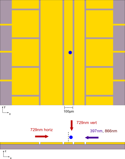
Figure 1: (color online) Schematic drawing of the asymmetric surface trap used in the experiments. The orientation of the cooling lasers is illustrated where the beams at wavelengths 397nm and 866nm perform Doppler cooling and the laser at 729nm enables sideband cooling close to the motional ground state. The expected trapping height is 107$\mu$m above the surface.

The noise polarization can be determined independently of the absolute noise magnitude by evaluating the ratio of the heating rates in two normal modes while rotating them. The black solid line in Fig. 2 shows the expected ratio of the heating rate of the two radial modes for the voltage independent noise model, leading to a maximum ratio of $R_{\rm indep}\approx 30.1$, which can be observed at an angle of $\phi_{\rm indep}\approx 17^{\circ}$. For the voltage dependent noise level and the set of voltages used in our setup, the maximum ratio is $R_{\rm dep}\approx 5.7$ for an angle $\phi_{\rm dep}\approx 50^{\circ}$.

Another possible noise source is electromagnetic pickup, which is expected to be largely common to all electrodes but the surrounding ground. Thus, the trap can be treated as a single electrode, resulting in an electric field pointing almost perpendicular to the trap surface with the maximum angle being close to 4^∘ and a maximum ratio of $R_{\textrm{pickup}}>10^{5}$. The angle deviating from zero is due to the asymmetric geometry of the electrodes.

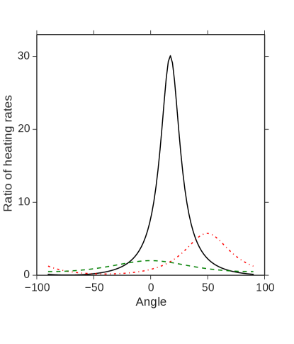
Figure 2: (color online) Ratio of the predicted heating rates in the two radial modes for various noise models. The green dashed line corresponds to surface noise, the black solid line corresponds to the voltage independent noise model and the red dashdotted line corresponds to the voltage dependent model.

III Measuring noise polarization

The polarization of the noise in an ion-trap can be estimated by measuring the heating rates of the normal modes while rotating the mode direction with respect to the trap surface. In order to reduce systematic errors in the measurements, it is advisable to perform all measurements at approximately the same mode frequency. Thus, it is beneficial to use the two radial modes, as their frequencies are close whereas the axial trap frequency is usually considerably smaller than any radial frequency. We denote the two normal radial modes $\updownarrow$ and $\leftrightarrow$, where the mode $\leftrightarrow$ shows an angle $\phi$ with respect to the trap surface. The heating rates for those two modes are given by

$$S_{\updownarrow}=S_{\rm max}\cos(\phi-\phi_{\rm max})^{2}+S_{\rm min}\sin(\phi-\phi_{\rm max})^{2}$$

$$S_{\leftrightarrow}=S_{\rm max}\sin(\phi-\phi_{\rm max})^{2}+S_{\rm min}\cos(\phi-\phi_{\rm max})^{2}\;,$$

where $S_{\rm max,min}$ is the maximum (minimum) noise amplitude and $\phi_{\rm max}$ is the angle where the maximum noise can be observed.

The radial trap modes can be rotated without affecting their frequencies by altering the static confinement. For this, the potential of each electrode $k$ is expanded in first and second order spherical harmonic expansion $U_{k}(\vec{r})\approx\sum_{i}C_{i,k}Y_{i}(\vec{r})$, where $C_{i,k}$ are the expansion coefficients and $Y_{i}(\vec{r})$ are the spherical harmonic functions Littich (2011); Allcock et al. (2010). We then find a set of voltages $V_{i,k}$ by finding solutions to the linear equation $\vec{e}_{i}=\sum_{k}C_{i,k}V_{i,k}$ with $\vec{e}_{i}$ being the basis vector corresponding to applying the spherical harmonic $Y_{i}(\vec{r})$. It is sufficient to consider only the spherical harmonic functions $Y_{0}(\vec{r})=z^{2}-x^{2}-y^{2}$, $Y_{1}(\vec{r})=x^{2}-y^{2}$ and $Y_{2}(\vec{r})=x\cdot y$. The functions $Y_{1,2}(\vec{r})$ allow control over the orientation of the radial trap axes as they correspond to a trapping configuration where the radial trap axes are aligned with the trap surface, $\phi_{1}=0^{\circ}$, or at $\phi_{2}=45^{\circ}$ respectively.

The orientation of the radial modes can be aligned to an arbitrary angle $\phi$ by applying a set of voltages that generates a potential with coefficients

$$C_{1}=C\,\cos(2\phi)$$

$$C_{2}=C\,\sin(2\phi)$$

where $C$ has to be large enough to overcome symmetry breaking due to stray fields. The resulting potential including the confinement in the axial direction is then:

$$U=C_{0}(x^{2}+y^{2}-2z^{2})+C_{1}(x^{2}-y^{2})+C_{2}(x\cdot y)+U_{\textrm{RF}}$$

with $C_{0}$ determining the strength of the axial confinement. The RF potential $U_{\textrm{RF}}$ and $Y_{0}$ have rotational symmetry around $z$ and thus do not affect the mode orientation.

In an asymmetric surface trap, such as shown in figure 1, it is also possible to rotate the radial trap axes by applying a static negative bias voltage onto the RF drive. This orients the trap axis of the higher frequency mode ($\updownarrow$) to $\phi_{g}$, which corresponds to the orientation where one of the normal modes is aligned with the field from the central electrode and hence close to the orientation of the maximum noise for voltage independent noise yielding an expected ratio of $R\approx 29.3$.

In order to estimate the ratio $R$, the heating rates of both radial modes need to be measured. The heating rates of a each mode can be inferred by comparing the relative strength of the blue and the red sideband after cooling the mode near the motional ground state Leibfried et al. (2003). Detecting these sidebands requires a geometry where the laser wave-vector has a considerable overlap with the respective mode axis. In order to provide this, we use the laser-beam geometry as sketched in figure 1. Having a laser beam perpendicular to the trap surface is not advisable when using a laser which causes charging on the trap surface Allcock et al. (2011); Harlander et al. (2010). Of particular concern is the laser light at 397 nm, required to prepare both modes at a reasonably low temperature to allow for sideband-cooling. To circumvent shining this light directly onto the trap, we apply a parametric coupling of the two modes Gorman et al. (2014).

The laser required to perform ground-state cooling and analysis of the final state has a wavelength of 729 nm which does not charge the trap surface notably Harlander et al. (2010). We also verified that the laser light does not affect the heating rate. We therefore can perform ground-state cooling and temperature analysis with a vertical 729 nm beam.

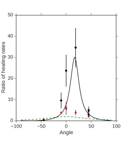
Figure 3: (color online) Measured ratio of the heating rate in the two radial modes. Red and blue diamonds are measurements without additional noise taken on different days. Black crosses are measurements with additional noise on the central electrode. The green dashed line corresponds to surface noise whereas the black solid line corresponds to the technical noise model.

We measured the heating rates in both modes while keeping the trap frequencies constant at $2.6\pm 0.1$  MHz. Figure 3 shows the heating rate as a function of the normal mode angle. For all but the angle $\phi_{g}$ the axes are rotated by controlling the static multipole confinement of all electrodes. For measuring at trap orientation with angle $\phi_{g}$, a static bias voltage is applied to the RF electrodes.

Applying this bias voltage on the RF electrodes allows for the most reliable trap rotation and thus we will only use this method for quantitative analysis of the noise polarization. We find a ratio of heating rates in the two modes of $R=4.2(5)$ which is small compared to the ratio predicted by the voltage independent noise model of $R\approx 30.1$. From this we can exclude the voltage independent technical noise model as the dominant noise source in our setup.

In order to exclude the voltage dependent noise model, we measure the heating rate for the $\updownarrow$ mode for two different sets of voltages providing an axial confinement of approximately 1 MHz (for set i) and 707 kHz (for set ii) while keeping the radial trap frequencies constant. The voltages of the sets differ by a factor of two and assuming the voltage noise to be proportional to the voltage, one would expect the heating rates to differ by a factor of four as the heating rate scales with the power spectral density of the noise. We measure a heating rate of $\dot{n}=0.69(6)$ quanta/ms for set i and $\dot{n}=0.52(3)$ quanta/ms for set ii, yielding a factor of 1.3(1) between the two heating rates. With this result we can exclude being dominated by noise that scales linearly with the applied voltage, as the model predicts a change in heating rate of a factor of four. A weaker scaling cannot be excluded completely but inferring a scaling factor would give no meaningful results due to large statistical uncertainties.

We further test the method by adding voltage noise to only the central electrode with a white noise generator. This should lead to an increase of the heating rate in the mode parallel to the maximum noise direction, whereas the perpendicular mode should not be affected. The experiments demonstrate this effect: The heating rate in the perpendicular mode without adding noise is $\dot{n}_{\leftrightarrow}=0.12(3)$ quanta/ms and with added noise $\dot{n}_{\leftrightarrow}=0.15(3)$ quanta/ms. In contrast, the measured heating rates in the perpendicular mode are $\dot{n}_{\updownarrow}=1.3(5)$ quanta/ms and with added noise $\dot{n}_{\updownarrow}=5.5(1)$ quanta/ms. This indicates that we can align the trap axes with the electric field generated by the center electrode (at angle $\phi_{g}$) with adequate precision.

IV Estimating surface noise in the presence of technical noise

Assuming a surface noise model featuring a ratio of $R_{\rm surf}=2$, we can estimate the magnitude of surface noise even in the presence of technical noise yielding a ratio $R_{\textrm{t}echn}$. It is convenient to perform the measurement at angle $\phi_{g}$ as this angle can be set with highest precision. Assuming that surface and technical noise are not correlated, the noise power spectral density is additive (the fields add in squares): $S_{\rm tot}=(S_{\rm surf}+S_{\rm techn})$ with $S_{\rm techn}$ originating from voltage independent technical noise. The ratio of the heating rates between both axes is measured and thus it is possible to estimate the magnitude of the surface noise as

$$S_{{\rm surf},\leftrightarrow}=S_{{\rm tot},\leftrightarrow}\,\frac{R_{\rm tot}-R_{\rm techn}}{R_{{\rm surf},\phi}-R_{\rm techn}}\;.$$

For the measured ratio $R_{\rm tot}=4.2(5)$ and the expected ratio for patch potentials $R_{{\rm surf},\phi}=R_{\rm surf}\cos{{}^{2}\phi}=2\,\cos{{}^{2}\phi}$, this leads to $S_{{\rm surf},\leftrightarrow}=1.8(2)\times 10^{-12}{\rm(V/m)^{2}/Hz}$. One needs to keep in mind that this noise amplitude is measured at the angle $\phi_{g}$. The surface noise magnitude parallel to the trap surface (along the x-axis) is then

$$S_{{\rm surf},x}=\frac{S_{{\rm surf},\leftrightarrow}}{R_{\rm surf}\sin(\phi)^{2}+\cos(\phi)^{2}}=\\ 1.7(2)\times 10^{-12}({\rm V/m})^{2}{/Hz}\;.$$ (2)

V Summary and conclusions

We studied the noise polarization and found a factor of 4.2(5)of the noise between the normal modes at an angle of $\phi_{g}$. If we assume a technical noise model where all electrodes show the same noise amplitude, we expect a factor of 30. From this we can exclude that the electric field noise parallel to the surface is dominated by such a noise source. An alternative noise model, where the noise depends on the applied voltage on the electrode, can lead to polarization similar to the one that is expected from surface noise. This noise model can be ruled out by comparing the noise magnitude for different applied voltages.

While it is certainly possible to construct technical noise models which explain our results by carefully choosing the amplitudes and correlations of the various voltage supplies, those models seem rather contrived. Assuming a simple and realistic technical noise model and a surface noise caused by either surface dipoles or fluctuating patch potentials, we can disentangle the contributions from technical noise and surface noise. From this we can conclude that, in our setup, technical noise is irrelevant to the field noise parallel to the trap surface, while its contribution in the vertical direction is comparable to surface noise. Using this method it will be possible to compare heating rates from different traps, allowing a meta-analysis of different experiments. We anticipate that this technique will be a useful tool towards solving the mystery behind the unexpected noise small ion traps suffer from Brownnutt et al. (2014).

References

- Kielpinski et al. (2002) D. Kielpinski, C. Monroe, and D. J. Wineland, Nature 417, 709 (2002).
- Turchette et al. (2000) Q. A. Turchette, Kielpinski, B. E. King, D. Leibfried, D. M. Meekhof, C. J. Myatt, M. A. Rowe, C. A. Sackett, C. S. Wood, W. M. Itano, C. Monroe, and D. J. Wineland, Phys. Rev. A 61, 63418 (2000).
- Monroe et al. (1995) C. Monroe, D. M. Meekhof, B. E. King, S. R. Jefferts, W. M. Itano, D. J. Wineland, and P. L. Gould, Phys. Rev. Lett. 75, 4011 (1995).
- Hite et al. (2012) D. A. Hite, Y. Colombe, A. C. Wilson, K. R. Brown, U. Warring, J. Jördens, J. D. Jost, K. S. McKay, D. P. Pappas, D. Leibfried, and D. J. Wineland, Phys Rev Lett 109, 103001 (2012).
- Daniilidis et al. (2011) N. Daniilidis, S. Narayanan, S. Möller, R. Clark, T. Lee, P. Leek, A. Wallraff, S. Schulz, F. Schmidt-Kaler, and H. Häffner, New J. Phys. 13, 013032 (2011).
- Allcock et al. (2011) D. T. C. Allcock, T. P. Harty, H. a. Janacek, N. M. Linke, C. J. Ballance, a. M. Steane, D. M. Lucas, R. L. Jarecki, S. D. Habermehl, M. G. Blain, D. Stick, and D. L. Moehring, Appl. Phys. B 107, 913 (2011).
- Deslauriers et al. (2006) L. Deslauriers, S. Olmschenk, D. Stick, W. K. Hensinger, J. Sterk, and C. Monroe, Phys. Rev. Lett. 97, 103007 (2006).
- Brownnutt et al. (2014) M. Brownnutt, M. Kumph, P. Rabl, and R. Blatt, ArXiv e-prints 1409.6572 (2014).
- Safavi-Naini et al. (2011) A. Safavi-Naini, P. Rabl, P. Weck, and H. Sadeghpour, Phys. Rev. A 84, 023412 (2011).
- Dubessy et al. (2009) R. Dubessy, T. Coudreau, and L. Guidoni, Phys. Rev. A 80, 031402 (2009).
- Wineland et al. (1998) D. J. Wineland, C. Monroe, W. M. Itano, D. Leibfried, B. E. King, and D. M. Meekhof, J. Res. Natl. Inst. Stand. Technol. 103, 259 (1998).
- Cirac and Zoller (1995) J. I. Cirac and P. Zoller, Phys. Rev. Lett. 74, 4091 (1995).
- Daniilidis et al. (2014) N. Daniilidis, S. Gerber, G. Bolloten, M. Ramm, A. Ransford, E. Ulin-Avila, I. Talukdar, and H. Häffner, Phys. Rev. B 89, 245435 (2014).
- Low et al. (2011) G. H. Low, P. Herskind, and I. Chuang, Phys. Rev. A 84, 053425 (2011).
- Martinis et al. (2005) J. Martinis, K. Cooper, R. McDermott, M. Steffen, M. Ansmann, K. Osborn, K. Cicak, S. Oh, D. Pappas, R. Simmonds, and C. Yu, Phys. Rev. Lett. 95, 1 (2005).
- Safavi-Naini et al. (2013) A. Safavi-Naini, E. Kim, P. Weck, P. Rabl, and H. Sadeghpour, Phys. Rev. A 87, 023421 (2013).
- Bowler et al. (2013) R. Bowler, U. Warring, J. W. Britton, B. C. Sawyer, and J. Amini, Rev. Sci. Instrum. 84, 033108 (2013).
- Baig et al. (2013) M. T. Baig, M. Johanning, A. Wiese, S. Heidbrink, M. Ziolkowski, and C. Wunderlich, Rev. Sci. Instrum. 84, 124701 (2013).
- Harlander et al. (2010) M. Harlander, M. Brownnutt, W. Hänsel, and R. Blatt, New J. Phys. 12, 093035 (2010).
- Poschinger et al. (2009) U. G. Poschinger, G. Huber, F. Ziesel, M. Deiss, M. Hettrich, S. A. Schulz, K. Singer, F. Schmidt-Kaler, G. Poulsen, M. Drewsen, and R. J. Hendricks, J. Phys. B At. Mol. Opt. Phys. 42, 154013 (2009).
- Littich (2011) G. Littich, Master’s thesis, ETH Zürich (2011).
- Allcock et al. (2010) D. T. C. Allcock, J. A. Sherman, D. N. Stacey, A. H. Burrell, M. J. Curtis, G. Imreh, N. M. Linke, D. J. Szwer, S. C. Webster, A. M. Steane, and D. M. Lucas, New J. Phys. 12, 053026 (2010).
- Leibfried et al. (2003) D. Leibfried, R. Blatt, C. Monroe, and D. Wineland, Rev. Mod. Phys. 75, 281 (2003).
- Gorman et al. (2014) D. J. Gorman, P. Schindler, S. Selvarajan, N. Daniilidis, and H. Häffner, Phys. Rev. A 89, 062332 (2014).