When Diabatic Trumps Adiabatic in Quantum Optimization

Abstract

We provide and analyze examples that counter the widely made claim that tunneling is needed for a quantum speedup in optimization problems. The examples belong to the class of perturbed Hamming-weight optimization problems. In one case, featuring a plateau in the cost function in Hamming weight space, we find that the adiabatic dynamics that make tunneling possible, while superior to simulated annealing, result in a slowdown compared to a diabatic cascade of avoided level-crossings. This, in turn, inspires a classical spin vector dynamics algorithm that is at least as efficient for the plateau problem as the diabatic quantum algorithm. In a second case whose cost function is convex in Hamming weight space, the diabatic cascade results in a speedup relative to both tunneling and classical spin vector dynamics.

The possibility of a quantum speedup for finding the solution of classical optimization problems is tantalizing, as a quantum advantage for this class of problems would provide a wealth of new applications for quantum computing. The goal of many optimization problems can be formulated as finding an $n$-bit string $x_{\mathrm{opt}}$ that minimizes a given function $f(x)$, which can be interpreted as the energy of a classical Ising spin system, whose ground state is $x_{\mathrm{opt}}$. Finding the ground state of such systems can be hard if, e.g., the system is strongly frustrated, resulting in a complex energy landscape that cannot be efficiently explored with any known algorithm due to the presence of many local minima Nishimori (2001). This can occur, e.g., in classical simulated annealing (SA) Kirkpatrick et al. (1983), when the system’s state is trapped in a local minimum. Provided the barriers between minima are sufficiently thin, quantum mechanics allows the system to tunnel in order to escape from such traps, though such comparisons must be treated with care since the quantum and classical potential landscapes are in general different. It is with this potential advantage over classical annealing that quantum annealing Ray et al. (1989); Finnila et al. (1994); Kadowaki and Nishimori (1998) and the quantum adiabatic algorithm (QA), were proposed Farhi et al. (2000). Thermal hopping and quantum tunneling provide two starkly different mechanisms for solving optimization problems, and finding optimization problems that favor the latter continues to be an open theoretical question S. Suzuki and A. Das (2015) (guest eds.); Heim et al. (2014). To attack this question, in this work we focus on a well-known class of problems known as perturbed Hamming weight oracle (PHWO) problems. These are problems for which instances can be generated where QA either has an advantage over classical random search algorithms with local updates, such as SA Farhi et al. (2002a); Reichardt (2004), or has no advantage van Dam et al. (2001); Reichardt (2004). Moreover, for PHWO problems with qubit permutation symmetry there is an elegant interpretation of tunneling in terms of a semiclassical potential Farhi et al. (2002a); Schaller and Schützhold (2010), which we exploit in this work.

If the total evolution time is sufficiently long so that the adiabatic condition is satisfied, QA is guaranteed to reach the ground state with high probability Jansen et al. (2007); Lidar et al. (2009). However, this condition is only sufficient, and the scaling of the time to reach the adiabatic regime is therefore not necessarily the right computational complexity metric. The optimal time to solution (TTS_opt), commonly used in benchmarking studies Rønnow et al. (2014) [also see the Supplementary Material (SM)], is a more natural metric. It is defined as the minimum total time such that the ground state is observed at least once with desired probability $p_{d}$:

$$\text{TTS}_{\mathrm{opt}}=\min_{t_{f}>0}\left(t_{f}\frac{\ln(1-p_{d})}{\ln\left(1-p_{\mathrm{GS}}(t_{f})\right)}\right)\ ,$$ (1)

where $t_{f}$ is the duration (in QA) or the number of single spin updates (in SA) of a single run of the algorithm, and $p_{\mathrm{GS}}(t_{f})$ is the probability of finding the ground state in a single such run. The use of TTS_opt allows for the possibility that multiple short (diabatic) runs of the evolution, each lasting an optimal annealing time $({t_{f}})_{\textrm{opt}}$, result in a better scaling than a single long (adiabatic) run with an unoptimized $t_{f}$.

Here we demonstrate that for a specific class of PHWO problems, the optimal evolution time $t_{f}$ for QA is far from being adiabatic, and this optimal evolution involves no multi-qubit tunneling. Instead the system leaves the ground state, only to return through a sequence of diabatic transitions associated with avoided-level crossings. We also show that spin vector dynamics, which can be interpreted as a semi-classical limit of the quantum evolution with a product-state approximation, evolves in an almost identical manner.

We note that PHWO problems are strictly toy problems since these problems are typically represented by highly non-local Hamiltonians (see the SM) and thus are not physically implementable, in the very same sense that the adiabatic Grover search problem is unphysical Roland and Cerf (2002); Rezakhani et al. (2010). Nevertheless, these problems provide us with important insights into the mechanisms behind a quantum speed-up, or lack thereof.

The plateau problem.—We focus on PHWO problems with a Hamiltonian of the form:

$$f(x)=\begin{cases}\left|x\right|+p(\left|x\right|)&l<\left|x\right|<u,\\ \left|x\right|&\text{elsewhere}\end{cases}\ ,$$ (2)

where $\left|x\right|$ denotes the Hamming weight of the bit string $x\in\{0,1\}^{n}$. The minimum of this function is $x_{\mathrm{opt}}=00\cdots 0$. In the absence of a perturbation, i.e., $p(\left|x\right|)=0$, the problem can be solved efficiently classically using a local spin-flip algorithm such as SA, since flipping any ‘$1$’ to a ‘$0$’ will lower the energy. Note that SA can be interpreted as a random walk, where the decision to walk left or right and flip a spin is given by the Metropolis update rule.

QA evolves the system from its ground state at $t=0$ according to a time-dependent Hamiltonian

$$H(s)=\frac{1}{2}\left(1-s\right)\sum_{i}\left(\openone-\sigma_{i}^{x}\right)+s\sum_{x}f(x)|x\rangle\langle x|\ ,$$ (3)

where we have chosen the standard transverse field “driver” Hamiltonian $H(0)$ that assumes no prior knowledge of the form of $f(x)$, and a linear interpolating schedule, with $s\equiv t/t_{f}$ being the dimensionless time parameter.

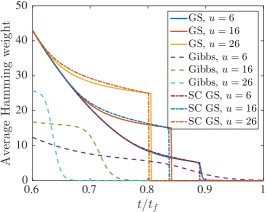
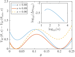
Figure 1: (a) $\mathinner{\langle{\mathrm{HW}}\rangle}$ in the instantaneous quantum ground state state (GS), the classical Gibbs state $\rho=e^{-\beta H_{Z}}/\mathcal{Z}$ (Gibbs), and the instantaneous quantum ground state predicted from the semi-classical potential (SC GS), as a function of their corresponding annealing parameters. The sharp drop in the GS and SC GS curves is due to a tunneling event wherein $\sim u$ qubits are flipped. Note that we use $t/t_{f}$ also for the Gibbs state, though in actuality the parameter is $\beta$, with a linear schedule: $\beta=0.1+5.9s$. (b) The semi-classical potential for $n=512$ and $u=6$ exhibits a double-well degeneracy at the position $s\approx 0.89$ (solid) of the sharp drop observed in (a), but is non-degenerate before and after this point (dotted and dashed), thus leading to a discontinuity in the position of its global minimum. The same is observed for other $u$ values we have checked (not shown). Inset: the difference in the position of the minimum gap from exact diagonalization and the position of the double-well degeneracy from the semi-classical potential, as a function of $n$, at $u=6$ (log-log scale).

Reichardt proved the following lower bound on the spectral gap for adiabatic evolutions for general PHWO problems Reichardt (2004):

$$\text{Gap}[H^{\text{pert}}(s)]\geq\text{Gap}[H^{\text{unpert}}(s)]-\mathcal{O}\left(h\frac{u-l}{\sqrt{l}}\right),$$ (4)

where $h=\max_{x}p(|x|)$ is the maximum height of the perturbation. Note that while the lower-bound holds for all perturbations, it is only non-trivial when it is positive for all $s\in[0,1]$. Details of our simulations methods and a summary of the proof are given in the SM.

We focus on the following “plateau” problem:

$$f(x)=\begin{cases}u-1&l<\left|x\right|<u,\\ \left|x\right|&\text{otherwise}\end{cases}\ .$$ (5)

Thus, here $h=u-l-1$. We note that when both $l,u=\mathcal{O}(1)$ a lower bound is not obtainable from Reichardt’s proof (this is explained in the SM), although numerical diagonalization reveals a constant gap. We demonstrate below that this case is nevertheless particularly hard for SA, and hence it is the focus of our study.

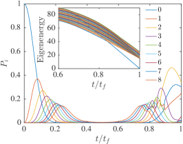
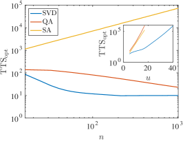
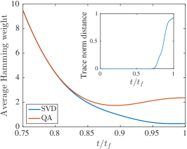
Figure 2: Diabatic QA vs SA and SVD. (a) Population $P_{i}$ in the $i$th energy eigenstate along the diabatic QA evolution at the optimal TTS for $n=512$ and $u=6$. Excited states are quickly populated at the expense of the ground state. By $t/t_{f}=0.5$ the entire population is outside the lowest $9$ eigenstates. In the second half of the evolution the energy eigenstates are repopulated in order. Inset: the eigenenergy spectrum along the evolution. Note the sequence of avoided level crossings that unmistakably line up in the spectrum to reach the ground state. (b) Scaling of the optimal TTS with $n$ for $u=6$, with an optimized number of single-spin updates for SA, and equal $({t_{f}})_{\textrm{opt}}$ for QA and SVD. SA scales as $\mathcal{O}(n)$, a consequence of performing sequential single-spin updates. QA and SVD both approach $\mathcal{O}(1)$ scaling as $n$ increases. Here we set $p_{d}=0.7$ in Eq. (1), in order to be able to observe the saturation of SVD’s TTS to the point where a single run suffices, i.e., TTS${}_{\textrm{opt}}=({t_{f}})_{\textrm{opt}}$. The conclusion is unchanged if we increase $p_{d}$: this moves the saturation point to larger $n$ for both SVD and QA, and we have checked that SVD always saturates before QA. Inset: scaling as a function of $u$ for $n=1008$. SVD is again seen to exhibit the best scaling, while for this value of $n$ the scaling of QA and SA is similar (QA’s scaling with $n$ improves faster than SA’s as a function of $n$, at constant $u$). (c) $\mathinner{\langle{\mathrm{HW}}\rangle}$ of the QA wavefunction and the SVD state (defined as the product of identical spin-coherent states) for $n=512$ and $u=6$. The behavior of the two is identical up to $t/t_{f}\approx 0.8$, when they begin to differ significantly, but neither displays any of the sharp changes observed in Fig. 1 for the instantaneous ground state. Inset: the trace-norm distance between the QA and SVD states, showing that they remain almost indistinguishable until $t/t_{f}\approx 0.8$.

Adiabatic dynamics.—We now demonstrate that, under the assumption of adiabatic dynamics, QA efficiently tunnels through a barrier and solves the plateau problem in at most linear time, while SA requires a time that grows polynomially in the problem size $n$.

In the adiabatic (long-time) limit, SA follows the thermal Gibbs state parametrized by the inverse temperature $\beta$, whereas QA follows the instantaneous ground state parametrized by $s$. We quantify the distance of these two states from the target (the $|0\rangle^{\otimes n}$ state) by calculating the expectation value of the Hamming weight operator, defined as $\mathrm{HW}=\frac{1}{2}\sum_{i=1}^{n}\left(\openone-\sigma^{z}_{i}\right)$. In particular, when $\mathinner{\langle{\mathrm{HW}}\rangle}\approx 0$, the system has a high probability of being in the state $|0\rangle^{\otimes n}$.

As we tune (the annealing parameters) $\beta$ and $s$, the plateau in Eq. (5) induces a dramatic change in $\mathinner{\langle{\mathrm{HW}}\rangle}$, of the order of the plateau width $u$ and over a narrow range of the annealing parameters, as shown in Fig. 1. For SA, traversing the plateau to reach the Gibbs state is a hard problem because, as the random walker moves closer to $x_{\mathrm{opt}}$, the probability to hop in the wrong direction of increasing Hamming weight becomes greater than the reverse. As we prove in the SM, consequently SA takes $\mathcal{O}(n^{u-l-1})$ single-spin updates to find the ground-state.

Unlike SA, to solve the plateau problem QA must tunnel through an energy barrier. To demonstrate this, we first construct the semiclassical effective potential arising from the spin-coherent path-integral formalism Klauder (1979):

$$V_{\mathrm{SC}}=\langle\theta,\phi|H(s)|\theta,\phi\rangle$$ (6)

where $|\theta,\phi\rangle$ are the spin-1/2 (symmetric) coherent states . The potential captures all the important features of the quantum Hamiltonian (3): it displays a degenerate double well potential almost exactly at the point of the minimum gap [see Fig. 1]; the discontinuous change in the position of the global minimum of the potential gives rise to a nearly identical change in $\mathinner{\langle{\textrm{HW}}\rangle}$ for the spin-coherent state [see Fig. 1]. This agreement improves with increasing $n$, which is expected from standard large-spin arguments Lieb (1973). The dramatic drop in $\mathinner{\langle{\textrm{HW}}\rangle}$ seen in Fig. 1 implies that $\sim u$ qubits have to be flipped in order to follow the instantaneous ground state. Since the double-well potential becomes degenerate at the point where this flipping happens, as seen in Fig. 1, QA tunnels through the barrier in order to adiabatically follow the ground state. The constant minimum gap implies that this tunneling event happens in a time that is dictated by the scaling of the numerator of the adiabatic condition. In our case this numerator turns out to be well approximated by the matrix element of $H(s)$ between the ground and first excited states, leading to $t_{f}\sim\mathcal{O}(n^{0.5})$ in the adiabatic limit (see the SM for details), thus polynomially outperforming SA whenever $u-l\geq 2$.

Optimal QA via Diabatic Transitions.—Even though QA encounters a constant gap and can tunnel efficiently, the possibility remains that this does not lead to an optimal TTS, since this result assumes the adiabatic limit. We thus consider a diabatic form of QA and next demonstrate, using the optimal TTS criterion defined in Eq. (1), that the optimal annealing time for QA is far from adiabatic. Instead, as shown in Fig. 2, the optimal TTS for QA is such that the system leaves the instantaneous ground state for most of the evolution and only returns to the ground state towards the end. The cascade down to the ground state is mediated by a sequence of avoided energy level-crossings. As $n$ increases for fixed $u$, repopulation of the ground state improves for fixed $({t_{f}})_{\textrm{opt}}$, hence causing TTS_opt to decrease with $n$, as seen Fig. 2, until it saturates to a constant at the lowest possible value, corresponding to a single run at $({t_{f}})_{\textrm{opt}}$. At this point the problem is solved in constant time $({t_{f}})_{\textrm{opt}}$, compared to the $\sim\mathcal{O}(n^{0.5})$ scaling of the adiabatic regime. Moreover, as shown in Fig. 2, there are no sharp changes in $\mathinner{\langle{\mathrm{HW}}\rangle}$, suggesting that the non-adiabatic dynamics do not entail multi-qubit tunneling events, unlike the adiabatic case.

Given the absence of tunneling in the time-optimal quantum evolution, we are motivated to consider a semiclassical limit of the evolution, particularly that of classical spin-vector dynamics (SVD), which we describe in detail in the SM. SVD can be derived as the saddle-point approximation to the path integral formulation of QA in the spin-coherent basis Owerre and Paranjape (2015). The equations share the same qubit permutation symmetry as the quantum Hamiltonian, which significantly simplifies the computation of the oracle [i.e., the potential (and its derivatives), now given by Eq. (6)] assumed for SVD. The SVD equations are equivalent to the Ehrenfest equations for the magnetization under the assumption that the density matrix is a product state, i.e., $\rho=\otimes_{i=1}^{n}\rho_{i}$, where $\rho_{i}$ denotes the state of the $i$th qubit.

As we show in Fig. 2, the scaling of SVD’s optimal TTS also saturates to a constant time, i.e., $({t_{f}})_{\textrm{opt}}$. Moreover, it reaches this value earlier (as a function of problem size $n$) than QA, thus outperforming QA for small problem sizes, while for large enough $n$ both achieve $\mathcal{O}(1)$ scaling. As seen in the inset, SVD’s advantage persists as a function of $u$ at constant $n$.

The dynamics of QA in the non-adiabatic limit are well approximated by SVD until close to the end of the evolution, as shown in Fig. 2: the trace-norm distance between the instantaneous states of QA and SVD is almost zero until $t/t_{f}\approx 0.8$, after which the states start to diverge. This suggests that SVD is able to replicate the QA dynamics up to this point, and only deviates because this makes it more successful at repopulating the ground state than QA.

Discussion.—For the class of PHWO problems studied here, we have demonstrated that tunneling is not necessary to achieve the optimal TTS. Instead, the optimal trajectory uses diabatic transitions to first scatter completely out of the ground state and return via a sequence of avoided level crossings. This use of diabatic transitions is similar in spirit to those studied in Refs. Somma et al. (2012); Crosson et al. (2014); Hen (2014); Steiger et al. (2015), but there are some important differences. essentially, our PHWO findings hold for the standard formulation of QA, without any fine-tuning of the interpolation schedule or the Hamiltonian. However, while both the adiabatic and diabatic quantum algorithms outperform SA for the plateau problem, the faster quantum diabatic algorithm is not better than the classical SVD algorithm for this problem. These results extend beyond the plateau problem: as we show in the SM even the “spike” problem studied in Ref. Farhi et al. (2002a)—which is in some sense the antithesis of the plateau problem since it features a sharp spike at a single Hamming weight—also exhibits the diabatic-beats-adiabatic phenomenon, indicating that tunneling is not required to efficiently solve the problem. Moreover, SVD is faster for this problem as well.

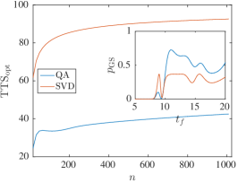
Figure 3: The optimal TTS for the potential given in Eq. (7). QA outperforms SVD over the range of problem sizes we were able to check. The reason can be seen in the inset, which displays the ground state probability for SVD and QA for different annealing times $t_{f}$, with $n=512$. The optimal annealing time for SVD occurs at the first peak in its ground state probability ($t_{f}\approx 8.98$), whereas the optimal annealing time for QA occurs at the much larger second peak in its ground state probability ($t_{f}\approx 10.91$).

However, the mechanism we found here, of a “lining-up” of the avoided level crossings with an associated “diabatic cascade” [seen in Fig. 2], may not be generic. E.g., we have checked that this mechanism is absent in the adiabatic Grover problem with a transverse field driver Hamiltonian [as in our Eq. (3)], even though the Grover problem is then equivalent to a “giant” plateau problem: $f(x)=1-\delta_{x,0}$ .

It is important to note that we do not claim that PHWO problems are always associated with diabatic cascades (see the SM for a counterexample); nor do we claim that SVD will always have an advantage over QA. A simple counterexample to the latter statement comes from the class of cost functions that are convex in Hamming weight space, which have a constant minimum gap Jarret and Jordan (2014):

$$f(x)=\begin{cases}2,&|x|=0\\ \left|x\right|,&\text{otherwise}\end{cases}\ .$$ (7)

We have observed similar diabatic transitions for this problem as for the plateau (not shown), thus obviating tunneling, but find that QA outperforms SVD, as shown in Fig. 3. This occurs because the optimum TTS for QA occurs at a slightly higher optimal annealing time, i.e., there is an advantage to evolving somewhat more slowly, though still far from adiabatically. Thus, this is a case of a “limited” quantum speedup Rønnow et al. (2014).

In summary, our work provides a counterargument to the widely made claim that tunneling is needed for a quantum speedup in optimization problems. Which features of Hamiltonians of optimization problems favor diabatic or adiabatic algorithms remains an open question.

Acknowledgements.—Special thanks to Ben Reichardt for insightful conversations and for suggesting the plateau problem, and to Bill Kaminsky for inspiring talks Kaminsky (2014a, b). We also thank Itay Hen, Joshua Job, Iman Marvian, Milad Marvian, and Rolando Somma for useful comments. The computing resources were provided by the USC Center for High Performance Computing and Communications and by the Oak Ridge Leadership Computing Facility at the Oak Ridge National Laboratory, which is supported by the Office of Science of the U.S. Department of Energy under Contract No. DE-AC05-00OR22725. This work was supported under ARO grant number W911NF-12-1-0523 and ARO MURI Grant No. W911NF-11-1-0268.

Supplementary Material for
“Diabatic Trumps Adiabatic in Quantum Optimization”

I Derivation of Eq. (1)

Equation (1) is easily derived as follows: the probability of successively failing $k$ times is $\left[1-p_{\mathrm{GS}}(t_{f})\right]^{k}$, so the probability of succeeding at least once after $k$ runs is $1-\left[1-p_{\mathrm{GS}}(t_{f})\right]^{k}$, which we set equal to the desired success probability $p_{d}$; from here one extracts the number of runs $k$ and multiplies by $t_{f}$ to get the time-to-solution TTS. Optimizing over $t_{f}$ yields TTS_opt, which is natural for benchmarking purposes in the sense that it captures the trade-off between repeating the algorithm many times vs optimizing the probability of success in a single run. The adiabatic regime might be more attractive if one seeks a theoretical guarantee to have a certain probability of success if the evolution is sufficiently slow.

II (Non-)Locality of PHWO problems

Since the PHWO problems, including the plateau, are quantum oracle problems, they can generically not be represented by a local Hamiltonian. For completeness we prove this claim here and also show why the (plain) Hamming weight problem is $1$-local.

Let $r$ be a bit string of length $n$, i.e., $r\in\{0,1\}^{n}$ and let

$$\sigma^{r}\equiv\sigma_{1}^{r_{1}}\otimes\sigma_{2}^{r_{2}}\otimes\dots\otimes\sigma_{n}^{r_{n}},$$ (8)

with $\sigma_{i}^{0}\equiv I_{i}$ and $\sigma_{i}^{1}\equiv\sigma_{i}^{z}$. This forms an orthonormal basis for the vector space of diagonal Hamiltonians. Thus:

$$H_{P}=\sum_{r\in\{0,1\}^{n}}J_{r}\sigma^{r},$$ (9)

with

$$J_{r} =\frac{1}{2^{n}}\mathrm{Tr}(\sigma^{r}H_{P})$$ (10a)

$$=\frac{1}{2^{n}}\sum_{x\in\{0,1\}^{n}}f(x)\langle x|\sigma^{r}|x\rangle$$ (10b)

$$=\frac{1}{2^{n}}\sum_{x\in\{0,1\}^{n}}f(x)(-1)^{x\cdot r}.$$ (10c)

Note that generically $J_{r}$ will be be non-zero for arbitrary-weight strings $r$, leading to $|r|$-local terms in $H_{P}$, even as high as $n$-local.

E.g., substituting the plateau Hamiltonian [Eq. (5)] into this we obtain:

$$J_{r} = \frac{1}{2^{n}}\left[\sum_{\left|x\right|\leq l\,\&\,\left|x\right|\geq u}\left|x\right|(-1)^{x\cdot r}\right.$$ (11)

$$\left.+(u-1)\sum_{l<\left|x\right|<u}(-1)^{x\cdot r}\right].$$

On the other hand, if $f(x)=|x|$ (i.e., in the absence of a perturbation), the Hamiltonian is only $1$-local:

$$H_{P} =\sum_{x\in\{0,1\}^{n}}|x||x\rangle\langle x|$$ (12a)

$$=\sum_{x_{1}=0}^{1}\dots\sum_{x_{n}=0}^{1}(x_{1}+x_{2}+\dots+x_{n})|x_{1}\rangle\langle x_{1}|$$

$$\hskip 56.9055pt\otimes|x_{2}\rangle\langle x_{2}|\otimes\dots\otimes|x_{n}\rangle\langle x_{n}|$$ (12b)

$$=\sum_{k=1}^{n}\left(x_{k}|x_{k}\rangle\langle x_{k}|\right)\bigotimes_{j\neq k}\left(\sum_{x_{j}=0}^{1}|x_{j}\rangle\langle x_{j}|\right)$$ (12c)

$$=\sum_{k=1}^{n}|1\rangle_{k}\langle 1|\bigotimes_{j\neq k}I_{j}=\sum_{k=1}^{n}|1\rangle_{k}\langle 1|.$$ (12d)

III Methods

III.1 Simulated Annealing

SA is a general heuristic solver Kirkpatrick et al. (1983), whereby the system is initialized in a high temperature state, i.e., in a random state, and the temperature is slowly lowered while undergoing Monte Carlo dynamics. Local updates are performed according to the Metropolis rule Metropolis et al. (1953); Hastings (1970): a spin is flipped and the change in energy $\Delta E$ associated with the spin flip is calculated. The flip is accepted with probability $P_{\mathrm{Met}}$:

$$P_{\mathrm{Met}}=\min\{1,\exp(-\beta\Delta E)\}\ ,$$ (13)

where $\beta$ is the current inverse temperature along the anneal. Note that there could be different schemes governing which spin is to be selected for the update. We consider two such schemes: random spin-selection – where the next spin to be updated is selected at random; and sequential spin-selection – where one runs through all of the $n$ spins in a sequence. Random spin-selection (including just updating nearest neighbors) satisfies detailed-balance and thus is guaranteed to converge to the Boltzmann distribution. Sequential spin-selection does not satisfy strict detailed balance (since the reverse move of sequentially updating in the reverse order never occurs), but it too converges to the Boltzmann distribution Manousiouthakis and Deem (1999). In sequential updating, a “sweep” refers to all the spins having been updated once. In random spin-selection, we define a sweep as the total number of spin updates divided by the total number of spins. When it is possible to parallelize the spin updates, the appropriate metric of time-complexity is the number of sweeps $N_{\mathrm{SW}}$, not the number of spin updates (they differ by a factor of $n$) Rønnow et al. (2014). However, in our problem this parallelization is not possible and hence the appropriate metric is the number of spin updates, and this is what is plotted in Fig. 2. After each sweep, the inverse temperature is incremented by an amount $\Delta\beta$ according to an annealing schedule, which we take to be linear, i.e. $\Delta\beta=(\beta_{f}-\beta_{i})/(N_{\mathrm{SW}}-1)$.

We can use SA both as an annealer and as a solver Hen et al. (2015). In the former, the state at the end of the evolution is the output of the algorithm, and can be thought of as a method to sample from the Boltzmann distribution at a specified temperature. For the latter, we select the state with the lowest energy found along the entire anneal as the output of the algorithm, the better technique if one is only interested in finding the global minimum. We use the latter to maximize the performance of the algorithm.

More details concerning the performance of SA in the context of the problem studied here are presented below.

III.2 Quantum Annealing

Here we consider the most common version of quantum annealing:

$$H(s)=(1-s)\sum_{i=1}^{n}\frac{1}{2}(\openone_{i}-\sigma_{i}^{x})+s\sum_{x\in\{0,1\}^{n}}f(x)|x\rangle\langle x|\ ,$$ (14)

where $s\equiv{t}/{t_{f}}$ is the dimensionless time parameter and $t_{f}$ is the total anneal time. The initial state is taken to be $|+\rangle^{\otimes n}$, which is the ground state of $H(0)$.

The initial ground state and the total Hamiltonian are symmetric under qubit permutations (recall that $f(x)=f(|x|)$ for our class of problems). It then follows that the time-evolved state, at any point in time, will also obey the same symmetry. Therefore the evolution is restricted to the $(n+1)$-dimensional symmetric subspace, a fact that we can take advantage of in our numerical simulations. This symmetric subspace is spanned by the Dicke states $|S,M\rangle$ with $S=n/2,M=-S,-S+1,\dots,S$, which satisfy:

$$S^{2}|S,M\rangle =S\left(S+1\right)|S,M\rangle$$ (15a)

$$S^{z}|S,M\rangle =M|S,M\rangle\ ,$$ (15b)

where $S^{x,y,z}\equiv\frac{1}{2}\sum_{i=1}^{n}\sigma_{i}^{x,y,z}$, $S^{2}=\left(S^{x}\right)^{2}+\left(S^{y}\right)^{2}+\left(S^{z}\right)^{2}$. We can denote these states by:

$$|w\rangle\equiv\left|\frac{n}{2},M=\frac{n}{2}-w\right>={n\choose w}^{-1/2}\sum_{x:|x|=w}|x\rangle,$$ (16)

where, $w\in\{0,\dots,n\}$.

In this basis the Hamiltonian is tridiagonal, with the following matrix elements:

$$\left[H(s)\right]_{w,w+1}= \left[H(s)\right]_{w+1,w}=$$

$$-\frac{1}{2}(1-s)\sqrt{(n-w)(w+1)},$$ (17a)

$$\left[H(s)\right]_{w,w}= (1-s)\frac{n}{2}+sf(w).$$ (17b)

The Schrödinger equation with this Hamiltonian can be solved reliably using an adaptive Runge-Kutte Cash-Karp method Cash and Karp (1990) and the Dormand-Prince method Dormand and Prince (1980) (both with orders $4$ and $5$).

If the quantum dynamics is run adiabatically the system remains close to the ground state during the evolution, and an appropriate version of the adiabatic theorem is satisfied. For evolutions with a constant spectral gap for all $s\in[0,1]$, an adiabatic condition of the form

$$t_{f}\geq\text{const}\sup_{s\in[0,1]}\frac{\|\partial_{s}H(s)\|}{\text{Gap}(s)^{2}}$$ (18)

is often claimed to be sufficient A. Messiah (1962) (however, see discussion after Eq. (21) in Ref. Jansen et al. (2007)). In our case $\|\partial_{s}H(s)\|=\|H(1)-H(0)\|$ is upper-bounded by $n$; since we are considering a constant gap, the adiabatic algorithm can scale at most linearly by condition (18). This is true for the plateau problems.

We demonstrate in SM-V that the following version of the adiabatic condition, known to hold in the absence of resonant transitions between energy levels Amin (2009), estimates the scaling we observe very well:

$$\max_{s\in[0,1]}\frac{|\langle\varepsilon_{0}(s)|\partial_{s}H(s)|\varepsilon_{1}(s)\rangle|}{\text{Gap}(s)^{2}}\ll 1,$$ (19)

where $\varepsilon_{0}(s)$ and $\varepsilon_{1}(s)$ are the instantaneous ground and excited states in the symmetric subspace respectively. To extract $t_{f}$ from this condition we simply ensure that for a given choice of $t_{f}$, condition (19) holds (recall that $s=t/t_{f}$).

III.3 Spin-Vector Dynamics

Starting with the spin-coherent path integral formulation of the quantum dynamics, we can obtain Spin Vector Dynamics (SVD) as the saddle-point approximation (see, for example, p.10 of Ref. Owerre and Paranjape (2015) or Refs. Smolin and Smith (2013); Albash et al. (2015)). It can be interpreted as a semi-classical limit describing coherent single qubits interacting incoherently. In this sense, SVD is a well motivated classical limit of the quantum evolution of QA. SVD describes the evolution of $n$ unit-norm classical vectors under the Lagrangian (in units of $\hbar=1$):

$$\mathcal{L}=i\mathinner{\langle{\Omega(s)|\frac{d}{ds}|\Omega(s)}\rangle}-t_{f}\mathinner{\langle{\Omega(s)|H(s)|\Omega(s)}\rangle},$$ (20)

where $|\Omega(s)\rangle$ is a tensor product of $n$ independent spin-coherent states Arecchi et al. (1972):

$$|\Omega(s)\rangle=\bigotimes_{i=1}^{n}\left[\cos\left(\frac{\theta_{i}(s)}{2}\right)|0\rangle_{i}+\sin\left(\frac{\theta_{i}(s)}{2}\right)e^{i\varphi_{i}(s)}|1\rangle_{i}\right].$$ (21)

We can define an effective semiclassical potential associated with this Lagrangian:

$$V_{\mathrm{SC}}(\{\theta_{i}\},\{\varphi_{i}\},s)\equiv\mathinner{\langle{\Omega(s)|H(s)|\Omega(s)}\rangle}$$

$$=(1-s)\sum_{i=1}^{n}\frac{1}{2}\left(1-\cos\varphi_{i}(s)\sin\theta_{i}(s)\right)$$

$$+s\sum_{x\in\{0,1\}^{n}}f(x)\prod_{j:x_{j}=0}\cos^{2}\left(\frac{\theta_{j}(s)}{2}\right)\prod_{j:x_{j}=1}\sin^{2}\left(\frac{\theta_{j}(s)}{2}\right),$$ (22)

with the probability of finding the all-zero state at the end of the evolution (which is the ground state in our case), as $\prod_{i=1}^{n}\cos^{2}\left(\frac{\theta_{i}(1)}{2}\right)$. The quantum Hamiltonian obeys qubit permutation symmetry: $PHP=H$ where $P$ is a unitary operator that performs an arbitrary permutation of the qubits. This implies that our classical Lagrangian obeys the same symmetry:

$$\mathcal{L}^{\prime} \equiv i\langle\Omega(s)|P\frac{d}{ds}P|\Omega(s)\rangle-t_{f}\langle\Omega(s)|PH(s)P|\Omega(s)\rangle$$

$$= i\langle\Omega(s)|\frac{d}{ds}|\Omega(s)\rangle-t_{f}\langle\Omega(s)|H(s)|\Omega(s)\rangle=\mathcal{L},$$

where the derivative operator is trivially permutation symmetric. Therefore, the Euler-Lagrange equations of motion derived from this action will be identical for all spins. Thus, if we have symmetric initial conditions, i.e., $(\theta_{i}(0),\varphi_{i}(0))=(\theta_{j}(0),\varphi_{j}(0))\ \forall i,j$, then the time evolved state will also be symmetric:

$$(\theta_{i}(s),\varphi_{i}(s))=(\theta_{j}(s),\varphi_{j}(s))\ \forall i,j\ \forall s\in[0,1]\ .$$ (24)

As we show below, under the assumption of a permutation-invariant initial condition we only need to solve two (instead of $2n$) semiclassical equations of motion:

$$\frac{n}{2}\sin\theta(s)\theta^{\prime}(s)-t_{f}\partial_{\varphi(s)}V_{\mathrm{SC}}^{\mathrm{sym}}(\theta(s),\varphi(s),s)=0\ ,$$ (25a)

$$-\frac{n}{2}\sin\theta(s)\varphi^{\prime}(s)-t_{f}\partial_{\theta(s)}V_{\mathrm{SC}}^{\mathrm{sym}}(\theta(s),\varphi(s),s)=0\ ,$$ (25b)

where we have defined the symmetric effective potential $V_{\mathrm{SC}}^{\mathrm{sym}}$ as:

$$V_{\mathrm{SC}}^{\mathrm{sym}}(\theta(s),\varphi(s),s)\equiv\mathinner{\langle{\Omega^{\mathrm{sym}}(s)|H(s)|\Omega^{\mathrm{sym}}(s)}\rangle}$$

$$=(1-s)\frac{n}{2}\left(1-\cos\varphi(s)\sin\theta(s)\right)$$

$$+s\sum_{w=0}^{n}f(w)\binom{n}{w}\sin^{2w}\left(\frac{\theta(s)}{2}\right)\cos^{2(n-w)}\left(\frac{\theta(s)}{2}\right),$$ (26)

and $|\Omega^{\mathrm{sym}}(s)\rangle$ is simply $|\Omega(s)\rangle$ with all the $\theta$’s and $\varphi$’s set equal. Note that in the main text [see Eq. (6)], we slightly abuse notation for simplicity, and use $V_{\mathrm{SC}}$ instead of $V_{\mathrm{SC}}^{\mathrm{sym}}$. The probability of finding the all-zero bit string at the end of the evolution is accordingly given by $\cos^{2n}(\theta(1)/2)$. We would have arrived at the same equations of motion had we used the symmetric spin coherent state in our path integral derivation, but that would have been an artificial restriction. In our present derivation the symmetry of the dynamics naturally imposes this restriction.

Note that the object in Eq. (III.3) involves a sum over all $2^{n}$ bit-strings and is thus exponentially hard to compute; on the other hand, the object in Eq. (III.3) only involves a sum over $n$ terms and is thus easy to compute. Therefore, just as in the quantum case—where due to permutation symmetry the quantum evolution is restricted to the $n+1$ dimensional subspace of symmetric states instead of the full $2^{n}$-dimensional Hilbert space—given knowledge of the symmetry of the problem we can efficiently compute the SVD potential and efficiently solve the SVD equations of motion.

We also remark that the computation of the potential in Eq. (III.3) is significantly simplified if our cost function, $f(x)$, is given in terms of a local Hamiltonian. For example, if $H(1)=\sum_{i,j}J_{ij}\sigma_{i}^{z}\sigma_{j}^{z}$, then:

$$V_{\mathrm{SC}}(\{\theta_{i}\},\{\varphi_{i}\},1)=\sum_{i,j}J_{ij}\cos\theta_{i}\cos\theta_{j}\ ,$$ (27)

which is easy to compute if is a $\mathrm{poly}(n)$ number of terms.

Let us now derive the symmetric SVD equations of motion (25). Without any restriction to symmetric spin-coherent states, the SVD equations of motion, for the pair $\theta_{i},\varphi_{i}$, read:

$$\frac{1}{2}\sin\theta_{i}(s)\theta_{i}^{\prime}(s)-t_{f}\partial_{\varphi_{i}(s)}V_{\mathrm{SC}}(\{\theta_{i}\},\{\varphi_{i}\},s)=0\ ,$$ (28a)

$$-\frac{1}{2}\sin\theta_{i}(s)\varphi_{i}^{\prime}(s)-t_{f}\partial_{\theta_{i}(s)}V_{\mathrm{SC}}(\{\theta_{i}\},\{\varphi_{i}\},s)=0\ .$$ (28b)

As can be seen by comparing Eqs. (25) and (28), it is sufficient to show that:

$$\frac{\partial}{\partial\theta_{i}}V_{\mathrm{SC}}\bigg{|}_{\theta_{j}=\theta,\varphi_{j}=\varphi\ \forall j}=\frac{1}{n}\frac{\partial}{\partial\theta}V_{\mathrm{SC}}^{\mathrm{sym}},$$ (29)

and an analogous statement holding for derivatives with respect to $\varphi$. This claim is easily seen to hold true for the term multiplying $(1-s)$ in Eq. (III.3):

$$\frac{\partial}{\partial\theta_{i}}\sum_{i=1}^{n}\frac{1}{2}\left(1-\cos\varphi_{i}(s)\sin\theta_{i}(s)\right)\bigg{|}_{\theta_{j}=\theta,\varphi_{j}=\varphi\ \forall j}$$

$$=\frac{\partial}{\partial\theta}\frac{1}{2}\left(1-\cos\varphi(s)\sin\theta(s)\right)$$

$$=\frac{1}{n}\frac{\partial}{\partial\theta}V_{\mathrm{SC}}^{\mathrm{sym}}(\theta,\phi,s=0)\ ,$$ (30)

where in the last line we used Eq. (III.3). Next we focus on the term multiplying $s$ in Eq. (III.3). This term has no $\varphi$ dependence and thus we only consider the $\theta$ derivatives. First note that

$$\frac{\partial}{\partial\theta_{i}}V_{\mathrm{SC}}(\{\theta_{i}\},\{\varphi_{i}\},s=1)=$$

$$\sum_{x\in\{0,1\}^{n}}f(x)\prod_{j:x_{j}=0}\cos^{2}\left(\frac{\theta_{j}}{2}\right)\prod_{j:x_{j}=1}\sin^{2}\left(\frac{\theta_{j}}{2}\right)$$

$$\times\left[-\delta_{x_{i},0}\sec^{2}\left(\frac{\theta_{i}}{2}\right)+\delta_{x_{i},1}\csc^{2}\left(\frac{\theta_{i}}{2}\right)\right]\frac{\sin\theta_{i}}{2}.$$ (31)

Now, we set all the $\theta_{i}$’s equal. Let us define $p(\theta)\equiv\sin^{2}\left(\frac{\theta}{2}\right)$. Using this and the fact that $f$ is only a function of the Hamming weight (which is equivalent to the qubit permutation symmetry), we can rewrite the last expression, after a few steps of algebra, as:

$$\sum_{w=0}^{n}f(w)p^{w-1}(1-p)^{n-w-1}\partial_{\theta}p$$

$$\hskip 85.35826pt\times\left[(1-p)\binom{n-1}{w-1}-p\binom{n-1}{w}\right]$$

$$=\sum_{w=0}^{n}f(w)p^{w-1}(1-p)^{n-w-1}\partial_{\theta}p\left[\frac{1}{n}\binom{n}{w}(w-np)\right]$$

$$=\frac{1}{n}\frac{\partial}{\partial\theta}V_{\mathrm{SC}}^{\mathrm{sym}}(\theta,\varphi,s=1)\ .$$ (32)

III.4 Simulated Quantum Annealing

Although not discussed in the main text, in SM-V we use an alternative method to simulated annealing, namely simulated quantum annealing (SQA, or Path Integral Monte Carlo along the Quantum Annealing schedule) Martoňák et al. (2002); Santoro et al. (2002). This is an annealing algorithm based on discrete-time path-integral quantum Monte Carlo simulations of the transverse field Ising model using Monte Carlo dynamics. At a given time $t$ along the anneal, the Monte Carlo dynamics samples from the Gibbs distribution defined by the action:

$$S[\mu]=\Delta(t)\sum_{\tau}H_{\mathrm{P}}(\mu_{:,\tau})-J_{\perp}(t)\sum_{i,\tau}\mu_{i,\tau}\mu_{i,\tau+1}$$ (33)

where $\Delta(t)=\beta B(t)/N_{\tau}$ is the spacing along the time-like direction, $J_{\perp}=-0.5\ln(\tanh(A(t)/2))$ is the ferromagnetic spin-spin coupling along the time-like direction, and $\mu$ denotes a spin configuration with a space-like direction (the original problem direction, indexed by $i$) and a time-like direction (indexed by $\tau$). For our spin updates, we perform Wolff cluster updates Wolff (1989) along the imaginary-time direction only. For each space-like slice, a random spin along the time-like direction is picked. The neighbors of this spin are added to the cluster (assuming they are parallel) with probability

$$P=1-\exp(-2J_{\perp})$$ (34)

When all neighbors of the spin have been checked, the newly added spins are checked. When all spins in the cluster have had their neighbors along the time-like direction tested, the cluster is flipped according to the Metropolis probability using the space-like change in energy associated with flipping the cluster. A single sweep involves attempting to update a single cluster on each space-like slice.

We can use SQA both as an annealer and as a solver Hen et al. (2015). In the former, we randomly pick one of the states on the Trotter slices at the end of the evolution as the output of the algorithm, while for the latter, we pick the state with the lowest energy found along the entire anneal as the output of the algorithm. We use the latter to maximize the performance of the algorithm.

IV Review of the Hamming weight problem and Reichardt’s bound for PHWO problems

Here we closely follow Ref. Reichardt (2004).

IV.1 The Hamming weight problem

We review the analysis within QA of the minimization of the Hamming weight function $f_{\mathrm{HW}}(x)=\left|x\right|$, which counts the number of $1$’s in the bit string $x$. This problem is of course trivial, and the analysis given here is done in preparation for the perturbed problem.

For the adiabatic algorithm, we start with the driver Hamiltonian,

$$H_{D}=\frac{1}{2}\sum_{i=1}^{n}\left(\openone_{i}-\sigma^{x}_{i}\right)=\sum_{i=1}^{n}|-\rangle_{i}\langle-|\ ,$$ (35)

which has $|+\rangle^{\otimes n}$ as the ground state.

The final Hamiltonian for the cost function $f_{\mathrm{HW}}(x)$ is

$$H_{P}=\frac{1}{2}\sum_{i=1}^{n}\left(\openone_{i}-\sigma^{z}_{i}\right)=\sum_{i=1}^{n}|1\rangle_{i}\langle 1|\ ,$$ (36)

which has $|0\rangle^{\otimes n}$ as the ground state.

We interpolate linearly between $H_{D}$ and $H_{P}$:

$$H(s) =(1-s)H_{D}+sH_{P};\quad s\in[0,1]$$ (37)

$$=\sum_{i=1}^{n}\frac{1}{2}\begin{pmatrix}1-s&-(1-s)\\ -(1-s)&1-s\end{pmatrix}_{i}+\begin{pmatrix}0&0\\ 0&s\end{pmatrix}_{i},$$ (38)

$$=\sum_{i=1}^{n}\frac{1}{2}\begin{pmatrix}1-s&-(1-s)\\ -(1-s)&1+s\end{pmatrix}_{i}\ .$$ (39)

Since there are no interactions between the qubits, this problem can be solved exactly by diagonalizing the Hamiltonian on each qubit separately. For each term, we have the energy eigenvalues $E_{\pm}(s)$,

$$E_{\pm}(s)=\frac{1}{2}(1\pm\Delta(s));\quad\Delta(s)\equiv\sqrt{1-2s+2s^{2}},$$ (40)

and associated eigenvectors,

$$|v_{\pm}(s)\rangle=\frac{1}{\sqrt{2\Delta(\Delta\mp s)}}\left[\mp(\Delta\mp s)|0\rangle+(1-s)|1\rangle\right]\ .$$ (41)

The ground state of $H(s)$ is $|v_{-}(s)\rangle^{\otimes n}$. The gap is given by,

$$\text{Gap}[H(s)] =H(s)|v_{+}(s)\rangle\otimes|v_{-}(s)\rangle^{\otimes(n-1)}$$

$$\hskip 85.35826pt-H(s)|v_{-}(s)\rangle^{\otimes n}$$ (42a)

$$=E_{+}+(n-1)E_{-}-nE_{-}$$ (42b)

$$=E_{+}-E_{-}$$ (42c)

$$=\Delta(s)\ .$$ (42d)

The gap is minimized at $s=\frac{1}{2}$ with minimum value $\Delta(\frac{1}{2})=\frac{1}{\sqrt{2}}$. The minimum gap is independent of $n$ and hence does not scale with problem size. Therefore the adiabatic run time is given by,

$$t_{f}=\mathcal{O}\left(\frac{\|H\|}{\Delta^{2}}\right)=\mathcal{O}(n)\ ,$$ (43)

where the $n$-dependence is solely due to $\|H\|$ (see SM-III.2).

It also useful to consider the form of $|v_{-}(s)\rangle^{\otimes n}$. We can write,

$$|v_{-}(s)\rangle^{\otimes n} = \frac{1}{[2\Delta(\Delta+s)]^{\frac{n}{2}}}\times$$ (44)

$$\sum_{x\in\{0,1\}^{n}}(1-s)^{\left|x\right|}(\Delta(s)+s)^{n-\left|x\right|}|x\rangle\ .$$

If we measure in the computational basis, the probability of getting outcome $x$ is determined by $\left|x\right|$:

$$\text{Pr}[x](s)=\left|\mathinner{\langle{v_{-}^{\otimes n}|x}\rangle}\right|^{2}=q(s)^{\left|x\right|}(1-q(s))^{n-\left|x\right|}\ ,$$ (45)

where

$$q(s)\equiv\frac{(1-s)^{2}}{[2\Delta(\Delta+s)]}\ .$$ (46)

IV.2 Reichardt’s bound for PHWO problems

Here we review Reichardt’s derivation of the gap lower-bound for general PHWO problems, but provide additional details not found in the original proof Reichardt (2004).

We use the same initial Hamiltonian [Eq. (35)] and linear interpolation schedule as before, $\tilde{H}(s)=(1-s)H_{D}+s\tilde{H}_{P}$, and choose the final Hamiltonian to be

$$\tilde{H}_{P}=\sum_{x\in\{0,1\}^{n}}\tilde{f}(x)|x\rangle\langle x|\ ,$$ (47)

where

$$\tilde{f}(x)=\begin{cases}\left|x\right|+p(x)&l<\left|x\right|<u\ ,\\ \left|x\right|&\text{elsewhere}\end{cases}\ ,$$ (48)

where $p(x)\geq 0$ is the perturbation. Note that here we have not assumed that the perturbation, $p(x)$, respects qubit permutation symmetry.

We wish to bound the minimum gap of $\tilde{H}(s)$. Unlike the Hamming weight problem $H(s)$, this problem is no longer non-interacting. Define

$$h_{k}\equiv\max_{\left|x\right|=k}p(x);\quad h\equiv\max_{k}h_{k}=\max_{x}p(x).$$ (49)

Lemma 1 (Reichardt (2004)).

Let $u=\mathcal{O}(l)$ and let $E_{0}(s)$ and $\tilde{E}_{0}(s)$ be the ground state energies of $H(s)$ and $\tilde{H}(s)$, respectively. Then $\tilde{E}_{0}(s)\leq E_{0}(s)+\mathcal{O}(h\frac{u-l}{\sqrt{l}})$.

Proof.

First note that

$$\tilde{H}(s)-H(s)=s\sum_{x:l<\left|x\right|<u}p(x)|x\rangle\langle x|\ .$$ (50)

Below, we suppress the $s$ dependence of all the terms for notational simplicity. We know that $E_{0}=\mathinner{\langle{v_{-}^{\otimes n}|H|v_{-}^{\otimes n}}\rangle}$. Using this,

$$\mathinner{\langle{\tilde{E}_{0}|\tilde{H}|\tilde{E}_{0}}\rangle} \leq\mathinner{\langle{\psi|\tilde{H}|\psi}\rangle}\quad\forall|\psi\rangle\in\mathcal{H}.$$ (51a)

$$\implies\tilde{E}_{0}-E_{0} \leq\mathinner{\langle{v_{-}^{\otimes n}|\tilde{H}|v_{-}^{\otimes n}}\rangle}-E_{0}$$ (51b)

$$\leq\mathinner{\langle{v_{-}^{\otimes n}|\tilde{H}-H|v_{-}^{\otimes n}}\rangle}$$ (51c)

$$=s\sum_{x:l<\left|x\right|<u}p(x)\left|\mathinner{\langle{v_{-}^{\otimes n}|x}\rangle}\right|^{2}$$ (51d)

$$=s\sum_{x:l<\left|x\right|<u}p(x)q^{\left|x\right|}(1-q)^{n-\left|x\right|}$$ (51e)

$$\leq\sum_{k:l<k<u}h_{k}{n\choose k}q^{k}(1-q)^{n-k},$$ (51f)

where ${n\choose k}$ is the number of strings with Hamming weight $k$, and we used Eq. (45).

Consider the partial binomial sum (dropping the $h_{k}$’s),

$$\sum_{k:l<k<u}{n\choose k}q^{k}(1-q)^{n-k}.$$ (52)

Using the fact that the binomial is well-approximated by the Gaussian in the large $n$ limit (note that this approximation requires that $q(s)$ and $1-q(s)$ not be too close to zero), we can write:

$$\sum_{k:l<k<u}{n\choose k}q^{k}(1-q)^{n-k}\approx\int_{l}^{u}d\xi\ \frac{1}{\sqrt{2\pi}\sigma}e^{-\frac{(\xi-\mu)^{2}}{2\sigma^{2}}}$$

$$\quad=\frac{1}{\sigma}\int_{l}^{u}d\xi\ \phi\left(\frac{\xi-\mu}{\sigma}\right)=\int_{(l-\mu)/\sigma}^{(u-\mu)/\sigma}dt\ \phi(t)\ ,$$ (53)

where $\quad\mu\equiv nq$, $\sigma\equiv\sqrt{nq(1-q)}$ and $\phi(t)\equiv\frac{e^{-t^{2}/2}}{\sqrt{2\pi}}$. Note that $\sigma$ and $\mu$ depend on $n$, and also on $s$ via $q(s)$. The parameters $l$ and $u$ are specified by the problem Hamiltonian, and are therefore allowed to depend on $n$ as long as $l(n)<u(n)<n$ is satisfied for all $n$.

Let us define:

$$B(s,n,l(n),u(n))\equiv\int_{(l(n)-\mu(n,s))/\sigma(n,s)}^{(u(n)-\mu(n,s))/\sigma(n,s)}dt\ \frac{e^{-t^{2}}/2}{\sqrt{2\pi}}.$$ (54)

We seek an upper bound on this function. We observe that $q(s)$ decreases monotonically from $\frac{1}{2}$ to $0$ as $s$ goes from $0$ to $1$. Thus, the mean of the Gaussian $\mu(n,s)=nq(s)$ decreases from $\frac{n}{2}$ to $0$. Depending on the values of $l(n)$, $u(n)$ and $\mu(n,s)$, we thus have three possibilities: (i) $l(n)<\mu(n,s)<u(n)$, (ii) $\mu(n,s)<l(n)<u(n)$, and (iii) $l(n)<u(n)<\mu(n,s)$. Note that (ii) and (iii) are cases where the integral runs over the tails of the Gaussian and so the integral is exponentially small. We focus on (i), as this induces the maximum values of the integral. In this case the lower limit of the integral Eq. (54) is negative, while the upper limit is positive. Thus, the integral runs through the center of the standard Gaussian, and we can upper-bound the value of the integral by the area of the rectangle of width $\frac{u(n)-l(n)}{\sigma(n,s)}$ and height $\frac{1}{\sqrt{2\pi}}$. Hence

$$B(s,n,l(n),u(n)) \leq\frac{1}{\sqrt{2\pi}}\frac{u(n)-l(n)}{\sigma(n,s)},$$ (55a)

$$=\frac{1}{\sqrt{2\pi}}\frac{u(n)-l(n)}{\sqrt{\mu(n)(1-q(s))}},$$ (55b)

$$\leq\frac{1}{\sqrt{2\pi}}\frac{u(n)-l(n)}{\sqrt{l(n)(1-q(s))}},$$ (55c)

where we have used the fact that $l(n)<\mu(n,s)=nq(s)$.

Thus, we obtain the bound:

$$\tilde{E}_{0}-E_{0}\leq\mathcal{O}\left(h\frac{u-l}{\sqrt{l}}\right).$$ (56)

∎

Lemma 2 (Reichardt (2004)).

If $\tilde{H}-H$ is non-negative, then the spectrum of $\tilde{H}$ lies above the spectrum of $H$. That is, $\tilde{E}_{j}\geq E_{j}$ for all $j$, where $\tilde{E}_{j}$ and $E_{j}$ denote the $j$th largest eigenvalue of $\tilde{H}$ and $H$, respectively.

This can be proved by a straightforward application of the Courant-Fischer min-max theorem (see, for example, Ref. Horn and Johnson (2012)).

Combining these lemmas results in the desired bound on the gap:

$$\text{Gap}[\tilde{H}(s)] =\tilde{E}_{1}-\tilde{E}_{0},$$ (57a)

$$\geq E_{1}-\tilde{E}_{0},$$ (57b)

$$=E_{1}-E_{0}-(\tilde{E}_{0}-E_{0}),$$ (57c)

$$\geq\Delta-\mathcal{O}\left(h\frac{u-l}{\sqrt{l}}\right),$$ (57d)

where in Eq. (57b) we used Lemma 2 and in Eq. (57d), we used Lemma 1.

Now, if we choose a parameter regime for the perturbation such that $h\frac{u-l}{\sqrt{l}}=o(1)$, then the perturbed problem maintains a constant gap. For example, if $l=\Theta(n)$ and $h(u-l)=\mathcal{O}(n^{1/2-\epsilon})$, for any $\epsilon>0$, then the gap is constant as $n\to\infty$.

V Adiabatic scaling

In order to study the adiabatic scaling, we consider the minimum time $\tau_{0}$ required to reach the ground state with some probability $p_{\mathrm{ThC}}$, where we choose $p_{\mathrm{ThC}}$ to ensure that we are exploring a regime close to adiabaticity for QA. We call this benchmark metric the “threshold criterion,” and set $p_{\mathrm{ThC}}=0.9$. As seen in Fig. 4, QA scales polynomially, approximately as $n^{0.5}$. It is also clear that the adiabatic criterion given by Eq. (19) provides an excellent proxy for the scaling of QA.

In light of a spate of recent negative results concerning the possibility of an advantage of SQA over SA (e.g., Ref. Heim et al. (2014)), it is remarkable, and of independent interest, that SQA scales better than SA for the plateau problem.

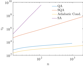
Figure 4: Log-log plot of the scaling of the time to reach a success probability of $0.9$, as a function of system size $n$ and $u=6$, for QA, SQA ($\beta=30$, $N_{\tau}=64$) and SA ($\beta_{f}=20$). The time for SQA and SA is measured in single-spin updates. We also show the scaling of the adiabatic condition as defined in Eq. (19) since it shows the same scaling as QA but can be calculated for larger spin systems. QA and the adiabatic condition scale approximately as $n^{0.5}$. SQA scales more favorably ($\sim n^{1.5}$) than SA ($\sim n^{5}$).

VI Analysis of simulated annealing using random spin selection

Here we analyze SA for the plateau and the Hamming weight problems. We consider a version of SA with random spin-selection as the rule that generates candidates for Metropolis updates.

An example of the plateau is illustrated in Fig. 5, with perturbation applied between strings of Hamming weight $3$ and $8$. Suppose we start from a random bit-string. For large $n$, with very high probability, we will start at a bit-string with Hamming weight close to $n/2$. The plateau may be to the left or to the right of $n/2$; if the plateau is to the right, then most likely the random walker will not encounter it and fall quickly to the ground state in at most $\mathcal{O}(n^{2})$ steps (see a few paragraphs below for a derivation).

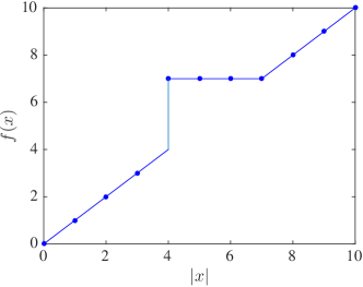
Figure 5: $l=3,u=8$

Thus, the interesting case is when the random walker arrives at the plateau from the right. In this case, how much time would it take, typically, for the walker to fall off the left edge? It is intuitively clear that traversing the plateau will be the dominant contribution to the time taken to reach the ground state, as after that the random walker can easily walk down the potential. As we show later below, this time can be at most $\mathcal{O}(n^{2})$ (ignoring transitions which take it back onto the plateau) for an inverse temperature that scales as $\beta=\Omega(\log n)$.

To evaluate the time to fall off the plateau, let us model the situation as follows. First, note that the perturbation is applied on strings of Hamming weight $l+1,l+2,\dots,u-1$, so the width of the plateau is $w=u-l-1$. Consider a random walk on a line of $w+1$ nodes labelled $0,1,\dots w$. Node $i$ represents the set of bit strings with Hamming weight $l+i$, with $0\leq i\leq w$. We assume that the random walker starts at node $w$, as it is falling onto the right edge of the plateau. Only nearest-neighbor moves are allowed and the walk terminates if the walker reaches node $0$.

Our model will estimate a shorter than actual time to fall off the left edge, because in the actual PHWO problem one can also go back up the slope on the right, and in addition we disallow transitions from strings of Hamming weight $l$ to $l+1$. This is justified because the Metropolis rule exponentially (in $\beta$) suppresses these transitions.

The transition probabilities $p_{i\to j}$ for this problem can be written as a $(w+1)\times(w+1)$ row-stochastic matrix $p_{ij}=p_{i\to j}$. $p$ is a tridiagonal matrix with zeroes on the diagonal, except at $p_{00}$ and $p_{ww}$. First consider $1\leq i\leq w-1$. If the walker is at node $i$, then its Hamming weight is $l+i$. Thus walker will move to $i+1$ (which has Hamming weight $l+i+1$) with probability $\frac{n-(l+i)}{n}$ (the chance that the bit picked had the value $0$). Now consider, $1\leq i\leq w$ the Hamming weight will decrease to $l+i-1$ with probability $\frac{l+i}{n}$ (the chance that the bit picked had the value $1$). Combining this with the fact that a walker at node $0$ stays put, we can write:

$$b_{i} \equiv p_{i\to i}=\begin{cases}1\text{ if }i=0\\ 0\text{ if }1\leq i\leq(w-1)\\ 1-\frac{l+w}{n}\text{ if }i=w\end{cases},$$ (58a)

$$c_{i} \equiv p_{i-1\to i}=\begin{cases}0\text{ if }i=1\\ 1-\frac{l+i-1}{n}\text{ if }i=2,\dots,w\end{cases},$$ (58b)

$$a_{i} \equiv p_{i\to i-1}=\frac{l+i}{n}\text{ if }i=1,2,\dots,w.$$ (58c)

Let $X(t)$ be the position of the random walker at time-step $t$. The random variable measuring the number of steps taken by the random walker starting from node $r$ would to reach node $s$ for the first time is

$$\tau_{r,s}\equiv\text{min}\{t>0:X(t)=s,X(t-1)\neq s|X(0)=r\}\ .$$ (59)

The quantity we are after is $\mathbb{E}\tau_{w,0}$, the expectation value of the random variable $\tau_{w,0}$, i.e., the mean time taken by the random walker to fall off the plateau. Since only nearest neighbor moves are allowed we have

$$\mathbb{E}\tau_{w,0}=\sum_{r=1}^{w}\mathbb{E}\tau_{r,r-1}\ .$$ (60)

Stefanov Stefanov (1995) (see also Ref. Krafft and Schaefer (1993)) has shown that

$$\mathbb{E}\tau_{r,r-1}=\frac{1}{a_{r}}\left(1+\sum_{s=r+1}^{w}\prod_{t=r+1}^{s}\frac{c_{t}}{a_{t}}\right),$$ (61)

where $c_{w+1}\equiv 0$. Evaluating the sum term by term:

$$\mathbb{E}\tau_{w,w-1} =\frac{n}{l+w},$$ (62a)

$$\mathbb{E}\tau_{w-1,w-2} =\frac{n}{l+w-1}\left[1+\frac{n-(l+w-1)}{l+w}\right],$$ (62b)

$$\mathbb{E}\tau_{w-2,w-3} =\frac{n}{l+w-2}\left[1+\frac{n-(l+w-2)}{l+w-1}\right.$$

$$\left.+\frac{n-(l+w-2)}{l+w-1}\times\frac{n-(l+w-1)}{l+w}\right],$$ (62c)

$$\vdots$$

$$\mathbb{E}\tau_{w-k,w-k-1} =\frac{n}{l+w-k}\left[1+\frac{n-(l+w-k)}{l+w-(k-1)}+\dots\right.$$

$$+\frac{n-(l+w-k)}{l+w-(k-1)}\times\cdots$$

$$\left.\times\frac{n-(l+w-2)}{l+w-1}\times\frac{n-(l+w-1)}{l+w}\right].$$ (62d)

Now consider the following cases:

1. $l,u=\mathcal{O}(1)$: Here, using the fact that $k=\mathcal{O}(w)=\mathcal{O}(1)$, we conclude that $\mathbb{E}\tau_{w-k,w-k-1}=\mathcal{O}(n^{k+1})$. Since the leading order term is $\mathbb{E}\tau_{w-(w-1),w-w}=\mathbb{E}\tau_{1,0}$, the time to fall off the plateau is $\mathcal{O}(n^{w})=\mathcal{O}(n^{u-l-1}).$

2. For Reichardt’s bound to give a constant lower-bound to the quantum problem, we need $u=l+o(l^{1/4})$. Since at most we can have $l=\mathcal{O}(n)$, we can conclude $\mathbb{E}\tau_{w-k,w-k-1}=\mathcal{O}\left(\frac{n}{l}\right)^{k+1}$. Therefore, the time to fall-off becomes $\mathbb{E}\tau_{w,0}=\mathcal{O}\left(w(\frac{n}{l})^{w}\right)$.

   • If $l=\Theta(n)$ and $w=\mathcal{O}(1)$, we can see that $\mathbb{E}\tau_{w,0}=\mathcal{O}(1)$, which is a constant time scaling.

   • If $l=\Theta(n)$ and $w=\mathcal{O}(n^{a})$, where $0<a<1/4$, then $\mathbb{E}\tau_{w,0}=\mathcal{O}(n^{a}\mathcal{O}(1)^{n^{a}})$, which is super-polynomial.

   • More generally, if $l=\mathcal{O}(n^{b})$, with $b\leq 1$ and $w=\mathcal{O}(n^{a})$, where $0\leq a<b/4$, then we get the scaling $\mathbb{E}\tau_{w,0}=\mathcal{O}(n^{a}\mathcal{O}(n^{1-b})^{n^{a}})$

Analysis of SA for plain Hamming weight — Let us analyze the behavior of a fixed temperature, i.e., there is no annealing schedule, simulated annealing on the plain Hamming weight problem. Here the transition probabilities are:

$$c_{i} \equiv p_{i-1\to i}=\frac{n-i+1}{n}e^{-\beta}\ ,$$ (63a)

$$a_{i} \equiv p_{i\to i-1}=\frac{i}{n}\ ,$$ (63b)

with $i=1,2,\dots,n$ denoting strings of Hamming weight $i$, and $\beta$ is the inverse temperature. Using the Stefanov formula (61), we can write (after much simplification):

$$\mathbb{E}\tau_{n-k,n-k-1}=\frac{n}{n-k}\binom{n}{k}^{-1}\sum_{l=0}^{k}e^{-l\beta}\binom{n}{k-l}\ .$$ (64)

Thus,

$$\mathbb{E}\tau_{n,0}=\sum_{k=0}^{n-1}\frac{n}{n-k}\binom{n}{k}^{-1}\sum_{l=0}^{k}e^{-l\beta}\binom{n}{k-l}\ .$$ (65)

This is the worst-case scenario as we are assuming that we start from the string of Hamming weight $n$, which is the farthest from the all-zeros string. Note that if we start from a random spin configuration, then with overwhelming probability, we will pick a string with Hamming weight close to $n/2$. Thus, most probably, $\mathbb{E}\tau_{n/2,0}$ will be the time to hit the ground state. We can write this as:

$$\mathbb{E}\tau_{n/2,0}=\sum_{k=n/2}^{n-1}\frac{n}{n-k}\binom{n}{k}^{-1}\sum_{l=0}^{k}e^{-l\beta}\binom{n}{k-l}.$$ (66)

We first show that $\beta=\mathcal{O}(1)$ will lead to an exponential time to hit the ground state. We show this by showing that $\mathbb{E}\tau_{1,0}$ is exponential if $\beta=\mathcal{O}(1)$. To this end,

$$\mathbb{E}\tau_{1,0} =\mathbb{E}\tau_{n-(n-1),n-n}$$ (67a)

$$=\sum_{l=0}^{n-1}e^{-l\beta}\binom{n}{n-1-l}$$ (67b)

$$=e^{\beta}\left[(e^{-\beta}+1)^{n}-1\right],$$ (67c)

which is clearly exponential in $n$ if $\beta=\mathcal{O}(1)$. Now let us suppose we have $\beta=\log n$, i.e. we decrease the temperature inverse logarithmically in system size. In this case,

$$\mathbb{E}\tau_{1,0}=n\left[\left(1+\frac{1}{n}\right)^{n}-1\right]\leq n(e-1)=\mathcal{O}(n)\ .$$ (68)

Now it is intuitively clear that $\mathbb{E}\tau_{1,0}>\mathbb{E}\tau_{r,r-1}$ for all $r>1$, which implies that $n\mathbb{E}\tau_{1,0}\geq\mathbb{E}\tau_{n,0}$. Thus, if $\beta=\log n$, then $\mathbb{E}\tau_{n,0}=\mathcal{O}(n^{2})$ at worst.

To obtain a lower-bound on the performance of the algorithm, we take $\beta\to\infty$. Thus, for each $k$ in Eq.(65), only the $l=0$ term will survive. Thus,

$$\lim_{\beta\to\infty}\mathbb{E}\tau_{n,0} =\sum_{k=0}^{n-1}\frac{n}{n-k}=n\sum_{i=1}^{n}\frac{1}{i}\approx n(\log n+\gamma)\ ,$$ (69)

for large $n$, with $\gamma$ as the Euler-Mascheroni constant. So the scaling here is $\mathcal{O}(n\log n)$. This is the best possible performance for single-spin update SA with random spin-selection on the plain Hamming weight problem. Therefore, if $\beta=\Omega(\log n)$, the scaling will be between $\mathcal{O}(n\log n)$ and $\mathcal{O}(n^{2})$.

To conclude, let us make a few remarks on the three different benchmarking metrics used in this work: (i) TTS_opt, (ii) the mean time to first hit the ground state ($\mathbb{E}\tau_{n/2,0}$ or $\mathbb{E}\tau_{n,0}$), and (iii) the time to cross a particular fixed threshold probability (typically high, say $p_{\mathrm{ThC}}=0.9$) of finding the ground state ($\tau_{\mathrm{ThC}}$). In order to compare the three, we would need to find TTS($t_{f}=\mathbb{E}\tau_{n/2,0}$) and TTS($t_{f}=\tau_{\mathrm{ThC}}$). By definition, TTS_opt, will be the smallest of the three. Further note that typically $p_{\mathrm{GS}}(t_{f}=\mathbb{E}\tau_{n/2,0})<p_{\mathrm{ThC}}$. This implies that if $t_{f}=\mathbb{E}\tau_{n/2,0}$, then the algorithm would need to be repeated more times than if $t_{f}=\tau_{\mathrm{ThC}}$ to obtain the same confidence that we have seen the ground state at least once. Note that either could have the smaller TTS, depending on the problem at hand.

We remark that the analysis performed above for random spin-selected SA with the complexity metric as $\mathbb{E}\tau_{n/2,0}$, captures extremely well the numerically obtained scaling of sequential spin-selected SA with the complexity metric as $\tau_{\mathrm{ThC}}$.

VII Other PHWO problems

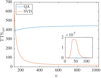
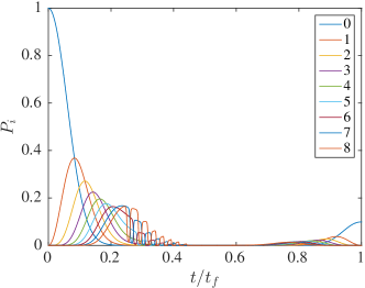
Figure 6: (a) The optimal TTS for the spike problem Farhi et al. (2002a). Inset: the optimal TTS for small problem sizes, where we observe SVD at first scaling poorly. However, as $n$ grows, this difficulty vanishes and it quickly beats QA. (b) We observe similar diabatic transitions for this problem (shown is $n=512$ and $t_{f}=9.85$) as we observed for the plateau [Fig. 2], although here the success probability appears to saturate faster than for the plateau problem.

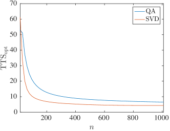
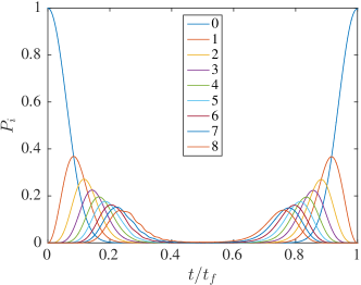
Figure 7: (a) The optimal TTS for the plateau with $l(n)=n/4$ and $u(n)=l(n)+6$. As can be seen, SVD is much better than QA for these problem sizes. (b) We observe similar diabatic cascades for this problem (shown is $n=512$ and $t_{f}=10$) as we observed for the plateau problem [Fig. 2].

In this section we consider several other versions of the PHWO problem. The first two examples exhibit diabatic cascades, while the last does not.

1. The “spike” problem studied by Farhi et al. Farhi et al. (2002a) has the following cost function:

   $$f(x)=\begin{cases}n,&\text{if }|x|=\frac{n}{4},\\ \left|x\right|,&\text{elsewhere}\end{cases}\ .$$ (70)

   This too is a problem designed explicitly to stymie SA (in Ref. Farhi et al. (2002a) it is argued that SA will take exponential time) and has polynomially decreasing gap $~{}\mathcal{O}(n^{-1/2})$ (and thus will have some polynomial run-time in the adiabatic regime). In Fig. 6 we show that this problem too shows diabatic cascades and a corresponding outperformance by SVD.

2. We pick an instance of the plateau with $l=n/4$ [i.e., $\mathcal{O}(n)$] and $u=l+6$ [i.e., $l+\mathcal{O}(1)$]. This problem has a constant lower-bound for QA by Reichardt’s theorem [see Eq. (4)], and SA is able to solve it in constant time [recall the discussion below Eq. (62)]. In Fig. 7, we see that this problem too exhibits diabatic transitions for QA and an advantage for SVD. For this problem, as we show in SM-VIII, the semiclassical effective potential asymptotically becomes identical to the unperturbed Hamming weight problem, which explains why the TTS_opt for this is decreasing: the TTS_opt for the (plain) Hamming weight problem is constant.

3. Consider the following class of PHWO problems, introduced in Ref. van Dam et al. (2001):

   $$f(x)=\begin{cases}p(|x|),&|x|>\left(\frac{1}{2}+\epsilon\right)\\ \left|x\right|,&|x|\leq\left(\frac{1}{2}+\epsilon\right)\end{cases}\ ,$$ (71)

   where $\epsilon>0$ and $p(\cdot)$ is a decreasing function which attains the global minimum, $-1$, in the $|x|>\left(\frac{1}{2}+\epsilon\right)$ region. Ref. van Dam et al. (2001) proved that this class of problems has an exponentially decreasing gap, and therefore the adiabatic algorithm would take exponentially long to find the ground state. We have considered the following instance of this class:

   $$f(x)=\begin{cases}-1,&|x|=n,\\ \left|x\right|,&\text{otherwise}\end{cases}\ .$$ (72)

   In this case, we did not observe the diabatic transition phenomenon (not shown), i.e., the optimal TTS is achieved by evolving adiabatically and remaining in the ground state. Thus the diabatic transition phenomenon does not persist for all PHWO problems.

VIII Asymptotic behavior of semiclassical effective potentials

Here we analyze the behavior of the (symmetric) effective potential we found in Eq. (III.3) and write down here in simplified form:

$$V_{\mathrm{SC}}(\theta,\varphi,s) \equiv\langle\theta,\varphi|H(s)|\theta,\varphi\rangle,$$

$$=\frac{n}{2}(1-s)(1-\sin\theta\cos\varphi)$$

$$\quad+s\sum_{w=0}^{n}f(w)\binom{n}{w}p(\theta)^{k}(1-p(\theta))^{n-k},$$ (73)

where $p(\theta)\equiv\sin^{2}\left(\frac{\theta}{2}\right)$. We take $f(w)$ to be a PHWO Hamiltonian of the form of Eq. (2). We can write the plateau’s effective potential as:

$$V_{\mathrm{SC}}^{\mathrm{pert}}=V_{\mathrm{SC}}^{{\mathrm{unpert}}}+s\sum_{l<k<u}f(k)\binom{n}{k}p(\theta)^{k}(1-p(\theta))^{n-k}.$$ (74)

Note the resemblance between the perturbation in the above equation and the term that appears in Reichardt’s lower-bound [see Eq. (51f)]. The only difference is that we have replaced $q(s)$ with $p(\theta)$. Now, if we trace through the arguments deriving the lower-bound on the gap, we see that the same holds for the perturbation term here. In particular:

$$\sum_{l<k<u}f(k)\binom{n}{k}p(\theta)^{k}(1-p(\theta))^{n-k}=\mathcal{O}\left(h\frac{u-l}{\sqrt{l}}\right).$$ (75)

Therefore, when $l,u=\mathcal{O}(1)$, the semiclassical effective potential asymptotically maintains a perturbation relative to the unperturbed problem. On the other hand, for the cases $l=\mathcal{O}(n),u=l+\mathcal{O}(1)$ and $l=\mathcal{O}(n),u=l+\mathcal{O}(n^{1/4-\epsilon})$, the perturbation to the semiclassical effective potential vanishes asymptotically. This shows that the effective potential leads to equivalent conclusions about computational hardness as the gap analysis.

IX Behavior of the average Hamming weight on the classical Gibbs state

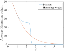
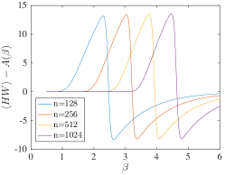
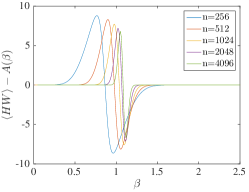
Figure 8: (a) $\langle\mathrm{HW}\rangle$ in the Gibbs state of the plain Hamming weight function and the plateau function with $l=0$ and $u=26$ for $n=128$. The two functions agree closely except in the region of the “drop.” (b) The “signal” $\mathinner{\langle{\mathrm{HW}}\rangle}-A(\beta)$ for $l=0,u=26$, for $n=128,256,512,1024$. The same sharp drop is seen for all $n$. (c) $\mathinner{\langle{\mathrm{HW}}\rangle}-A(\beta)$ for the case $l(n)=n/4,u(n)=l(n)+26$, for $n=256,512,1024,2048,3200,4096$. Here the drop is slowly decreasing with $n$.

In this section we expand on the behavior of the average Hamming weight $\mathinner{\langle{\mathrm{HW}}\rangle}$ for different cases of the plateau problem.

In Fig. 1, we plotted $\mathinner{\langle{\mathrm{HW}}\rangle}$ for the classical Gibbs state as a function of the inverse temperature, $\beta$. We interpreted the sharp drops in this quantity as a sign that the problem becomes hard for SA. To understand this better we can consider these sharp drops as modifications of the smooth behavior [see Fig. 8] of the plain Hamming weight function, i.e., Eq. (2) with $p(\left|x\right|)=0$. For this case:

$$A(\beta)\equiv\mathinner{\langle{\mathrm{HW}}\rangle}_{\mathrm{HamWt}}=\frac{ne^{-\beta}}{1+e^{-\beta}}.$$ (76)

In order to study just the “drop,” we subtract $A(\beta)$ as the “background,” and focus our attention on the “signal,” which is the sharp change.

We consider the following two varieties of the plateau:

1. $l,u=\mathcal{O}(1)$. This was the case studied in the main text, and we proved above that in this case SA requires polynomial time. As we can see from Fig. 8, the sharpness of the drop remains constant with increasing $n$. This is consistent with the problem being hard for SA.

2. $l=\mathcal{O}(n)$ and $u=l+\mathcal{O}(1)$. Reichardt’s lower bound applies in this case, and we proved above that this case is solved in time $\mathcal{O}(1)$ by SA. As can be seen in Fig. 8 the sharpness of the drop decreases (albeit slowly) with $n$. This is consistent with the problem being easy for SA.

To conclude we remark on another case which has constant gap lower-bound by Reichardt’s proof. Here, $l=\mathcal{O}(n),u=l+\mathcal{O}(n^{1/4-\epsilon})$, $\epsilon>0$. We do not find any dramatic changes in the instantaneous quantum ground state during the evolution as in Fig. 1, suggesting that multi-qubit tunneling does not play a significant role, hence making it a less relevant problem for our discussion.

References

- Nishimori (2001) H. Nishimori, Statistical Physics of Spin Glasses and Information Processing: An Introduction (Oxford University Press, Oxford, UK, 2001).
- Kirkpatrick et al. (1983) S. Kirkpatrick, C. D. Gelatt, and M. P. Vecchi, Science 220, 671 (1983).
- Ray et al. (1989) P. Ray, B. K. Chakrabarti, and A. Chakrabarti, Phys. Rev. B 39, 11828 (1989).
- Finnila et al. (1994) A. Finnila, M. Gomez, C. Sebenik, C. Stenson, and J. Doll, Chemical Physics Letters 219, 343 (1994).
- Kadowaki and Nishimori (1998) T. Kadowaki and H. Nishimori, Phys. Rev. E 58, 5355 (1998).
- Farhi et al. (2000) E. Farhi, J. Goldstone, S. Gutmann, and M. Sipser, arXiv:quant-ph/0001106 (2000).
- S. Suzuki and A. Das (2015) (guest eds.) S. Suzuki and A. Das (guest eds.), Eur. Phys. J. Spec. Top. 224, 1 (2015).
- Heim et al. (2014) B. Heim, T. F. Rønnow, S. V. Isakov, and M. Troyer, arXiv:1411.5693 (2014).
- Farhi et al. (2002a) E. Farhi, J. Goldstone, and S. Gutmann, arXiv:quant-ph/0201031 (2002a).
- Reichardt (2004) B. W. Reichardt, in Proceedings of the Thirty-sixth Annual ACM Symposium on Theory of Computing, STOC ’04 (ACM, New York, NY, USA, 2004) pp. 502–510.
- van Dam et al. (2001) W. van Dam, M. Mosca, and U. Vazirani, Foundations of Computer Science, 2001. Proceedings. 42nd IEEE Symposium on, Foundations of Computer Science, 2001. Proceedings. 42nd IEEE Symposium on , 279 (8-11 Oct. 2001).
- Schaller and Schützhold (2010) G. Schaller and R. Schützhold, Quantum Information & Computation 10, 0109 (2010).
- Jansen et al. (2007) S. Jansen, M.-B. Ruskai, and R. Seiler, J. Math. Phys. 48, (2007).
- Lidar et al. (2009) D. A. Lidar, A. T. Rezakhani, and A. Hamma, J. Math. Phys. 50, (2009).
- Rønnow et al. (2014) T. F. Rønnow, Z. Wang, J. Job, S. Boixo, S. V. Isakov, D. Wecker, J. M. Martinis, D. A. Lidar, and M. Troyer, Science 345, 420 (2014).
- Roland and Cerf (2002) J. Roland and N. J. Cerf, Phys. Rev. A 65, 042308 (2002).
- Rezakhani et al. (2010) A. T. Rezakhani, A. K. Pimachev, and D. A. Lidar, Phys. Rev. A 82, 052305 (2010).
- Klauder (1979) J. R. Klauder, Physical Review D 19, 2349 (1979).
- Note (1) The semiclassical potential has been used profitably in various QA studies, e.g., Refs. Farhi et al. (2002a); Schaller and Schützhold (2010); Farhi et al. (2002b); Boixo et al. (2014).
- Lieb (1973) E. H. Lieb, Communications in Mathematical Physics 31, 327 (1973).
- Owerre and Paranjape (2015) S. Owerre and M. Paranjape, Physics Reports 546, 1 (2015).
- Somma et al. (2012) R. D. Somma, D. Nagaj, and M. Kieferová, Phys. Rev. Lett. 109, 050501 (2012).
- Crosson et al. (2014) E. Crosson, E. Farhi, C. Y.-Y. Lin, H.-H. Lin, and P. Shor, arXiv preprint arXiv:1401.7320 (2014).
- Hen (2014) I. Hen, Journal of Physics A: Mathematical and Theoretical 47, 045305 (2014).
- Steiger et al. (2015) D. S. Steiger, T. F. Rønnow, and M. Troyer, arXiv:1504.07991 (2015).
- Note (2) Note that this is not the version of the Grover problem that admits a quantum speedup, as this requires a rank- driver Hamiltonian Roland and Cerf (2002)).
- Jarret and Jordan (2014) M. Jarret and S. P. Jordan, Journal of Mathematical Physics 55, 052104 (2014).
- Kaminsky (2014a) W. M. Kaminsky, in Quantum Optimization Workshop (The Fields Institute for Research in Mathematical Sciences, 2014).
- Kaminsky (2014b) W. M. Kaminsky, “Diabatic Quantum Computation – Why it Might Not Really Pay to Go for the “A”?” USC Quantum Information Seminar (2014b).
- Farhi et al. (2002b) E. Farhi, J. Goldstone, and S. Gutmann, arXiv:quant-ph/0208135 (2002b).
- Boixo et al. (2014) S. Boixo, V. N. Smelyanskiy, A. Shabani, S. V. Isakov, M. Dykman, V. S. Denchev, M. Amin, A. Smirnov, M. Mohseni, and H. Neven, arXiv:1411.4036 (2014).
- Metropolis et al. (1953) N. Metropolis, A. W. Rosenbluth, M. N. Rosenbluth, A. H. Teller, and E. Teller, J. Chem. Phys. 21, 1087 (1953).
- Hastings (1970) W. K. Hastings, Biometrika 57, 97 (1970).
- Manousiouthakis and Deem (1999) V. I. Manousiouthakis and M. W. Deem, J. Chem. Phys. 110, 2753 (1999).
- Hen et al. (2015) I. Hen, J. Job, T. Albash, T. F. Rønnow, M. Troyer, and D. Lidar, arXiv:1502.01663 (2015).
- Cash and Karp (1990) J. R. Cash and A. H. Karp, ACM Trans. Math. Softw. 16, 201 (1990).
- Dormand and Prince (1980) J. Dormand and P. Prince, Journal of Computational and Applied Mathematics 6, 19 (1980).
- A. Messiah (1962) A. Messiah, Quantum Mechanics, Vol. 2 (North-Holland, Amsterdam, 1962).
- Amin (2009) M. H. S. Amin, Phys. Rev. Lett. 102, 220401 (2009).
- Smolin and Smith (2013) J. A. Smolin and G. Smith, arXiv:1305.4904 (2013).
- Albash et al. (2015) T. Albash, T. F. Rønnow, M. Troyer, and D. A. Lidar, Eur. Phys. J. Spec. Top. 224, 111 (2015).
- Arecchi et al. (1972) F. Arecchi, E. Courtens, R. Gilmore, and H. Thomas, Physical Review A 6, 2211 (1972).
- Martoňák et al. (2002) R. Martoňák, G. E. Santoro, and E. Tosatti, Phys. Rev. B 66, 094203 (2002).
- Santoro et al. (2002) G. E. Santoro, R. Martoňák, E. Tosatti, and R. Car, Science 295, 2427 (2002).
- Wolff (1989) U. Wolff, Phys. Rev. Lett. 62, 361 (1989).
- Horn and Johnson (2012) R. A. Horn and C. R. Johnson, Matrix Analysis (Cambridge University Press, 2012).
- Stefanov (1995) V. T. Stefanov, Journal of Applied Probability , 846 (1995).
- Krafft and Schaefer (1993) O. Krafft and M. Schaefer, Journal of Applied Probability 30, 964 (1993).