CP-odd contributions to the $ZZ^{*}\gamma$, $ZZ\gamma^{*}$, and $ZZZ^{*}$ vertices induced by nondiagonal charged scalar boson couplings

Abstract

In models with extended scalar sectors with several Higgs multiplets, such as Higgs triplet models, the $Z$ gauge boson can have nondiagonal couplings to charged Higgs bosons. In a model-independent way, we study the potential contributions arising from such theories to the CP-violating trilinear neutral gauge boson couplings $ZZ^{*}\gamma$, $ZZ\gamma^{*}$, and $ZZZ^{*}$, which are parametrized by four form factors: $h^{Z}_{1,2}$, $f_{4}^{\gamma}$, and $f_{4}^{Z}$, respectively. Such form factors can only be induced if there are at least two nondegenerate charged Higgs scalars and an imaginary phase in the coupling constants. For the masses of the charged scalar bosons we consider values above 300 GeV and find that the form factors can reach the following orders of magnitude: $|h_{1}^{Z}|\sim 10^{-5}-10^{-4}$, $|h_{2}^{Z}|\sim 10^{-7}-10^{-6}$, $|f_{4}^{\gamma}|\sim 10^{-5}-10^{-3}$ and $|f_{4}^{Z}|\sim 10^{-6}-10^{-5}$, though there could be an additional suppression factor arising from the coupling constants. We also find that the form factors decouple at high energies and are not very sensitive to a change in the masses of the charged scalar bosons. Apart from a proportionality factor, our results for the $f_{4}^{Z}$ form factor, associated with the $ZZZ^{*}$ vertex, is of the same order of magnitude than that induced via nondiagonal neutral scalar boson couplings in the framework of a two-Higgs doublet model.

I Introduction

Pair production of electroweak gauge bosons ($W$, $Z$ and $\gamma$) provides an import test for the gauge sector of the standard model (SM), and opens up the possibility for observing new physics phenomena associated with such particles. In this context, the production of a pair of neutral gauge bosons, $Z\gamma$ or $ZZ$, was studied at LEP Achard et al. (2004); Abdallah et al. (2007), Tevatron Abazov et al. (2007, 2008, 2012) and the LHC Aad et al. (2012a, 2013a); Chatrchyan et al. (2013a, b). The main production mechanism proceeds at leading order via the $t$ and $u$ channels, but regardless of the production process, the experimental measurements were found to be consistent with the SM predictions Achard et al. (2004); Abdallah et al. (2007); Abazov et al. (2007, 2008, 2012); Aad et al. (2012a, 2013a); Chatrchyan et al. (2013a, b). Any deviation in the corresponding cross sections could be a hint of new physics effects, such as new heavy particles Cortes Maldonado et al. (2012), new interactions Kober et al. (2007); Baur and Rainwater (2000), etc. In particular, $Z\gamma$ and $ZZ$ production could allow us to study the trilinear neutral gauge boson couplings (TNGBCs) $ZV_{i}V_{j}$, whose framework is best discussed via the effective Lagrangian approach, as in Ref. Larios et al. (2001), where the lowest-dimension effective operators inducing the off-shell TNGBcs were presented. Since the $\gamma\gamma\gamma$ coupling is forbidden by Furry’s theorem, experimentalists have focused their attention on the $Z\gamma\gamma$, $ZZ\gamma$ and $ZZZ$ couplings. On the other hand, Landau-Yang’s theorem forbids any TNGBC with three on-shell gauge bosons, so there are only two vertex functions describing four distinct TNGBCs with one off-shell gauge boson: $ZV^{*}\gamma$ and $ZZV^{*}$ ($V=\gamma$, $Z$) Hagiwara et al. (1987). The most general $ZV^{*}\gamma$ vertex function fulfilling both Lorentz and electromagnetic gauge invariance is parametrized in terms of four forms factors $h_{i}^{V}$ ($i=1,2,3,4$), whereas the $ZZV^{*}$ vertex function is parametrized by only two forms factors $f_{j}^{V}$ ($j=4,5$). While $h_{1,2}^{V}$ and $f_{4}^{V}$ are CP violating, $h_{3,4}^{V}$ and $f_{5}^{V}$ are CP conserving. Any TNGBC is zero at the tree level in the SM or any renormalizable extension, only the CP-conserving ones are non-vanishing at the one-loop level in the SM via the fermion triangle Gounaris et al. (2000a), whose contribution is highly suppressed even in the presence of a fourth fermion family Hernandez et al. (1999). The respective experimental bounds on TNGBCs are expected to achieve a significant improvement in the LHC in the forthcoming years. Thus, it is worth studying any possible contribution to these couplings at a high energy scale $\Lambda$ via effective Lagrangian.

Although the CP violation observed in the $K$ meson system can be explained by the Cabibbo-Kobayashi-Maskawa matrix complex phase, the SM does not predicts enough CP violating effects to explain the current matter-antimatter asymmetry in the universe. Consequently, other sources of CP violation are necessary. Such CP-violating effects may show up via TNGBCs, which are thus worth studying. Along these lines, it was shown that the radiative decay $Z\to\mu^{+}\mu^{-}\gamma$ may be sensitive to both CP-conserving and CP-violating $ZV^{*}\gamma$ and $ZZV^{*}$ TNGBCs. Furthermore, such a process may also be useful to put constraints on the CP-violating forms factors in future linear collider experiments Perez and Ramirez-Zavaleta (2005). The current experimental bounds on TNGBCs reported by the PDG collaboration Beringer et al. (2012) come from a combination of LEP measurements ALEPH:2005aa (697356), where the experimental results and the individual analyses are based in reports between 1999 and 2001. However, the L3 collaboration has updated their analyses, resulting in the most restrictive bound on $h_{1,2}^{V}$ up to date Achard et al. (2004). On the other hand, a few results have been reported by the CMS Chatrchyan et al. (2013a, b) and ATLAS collaborations Aad et al. (2012a, 2013a). The current most stringent bound on $f_{4}^{V}$ was obtained by CMS Chatrchyan et al. (2013a), based on data collected in 2010 and 2011 at $\sqrt{s}=7$ TeV with an integrated luminosity of $5.0\pm 0.1$ fb^-1. A more accurate analysis is expected by both the ATLAS and the CMS collaborations in the forthcoming years. The most stringent bounds on the TNGBCs form factors are shown in Table 1.

Experiment	Limit
L3 Achard et al. (2004)	$-0.153<h_{1}^{Z}<0.141$
L3 Achard et al. (2004)	$-0{.}087<h_{2}^{Z}<0{.}079$
CMS Chatrchyan et al. (2013a)	$-0{.}011<f_{4}^{Z}<0.012$
CMS Chatrchyan et al. (2013a)	$-0.013<f_{4}^{\gamma}<0.015$

Table 1: The current most stringent limits on CP-violating TNGBCs.

Contributions to TNGBCs have been previously studied in the context of the minimal supersymmetric standard model (MSSM) Choudhury et al. (2001) and the littlest Higgs model Dutta et al. (2009), focusing only on the CP-conserving form factors. Moreover, the CP-violating $ZZZ^{*}$ form factors were studied in the framework of two-Higgs doublet model (THDM), where the respective contributions are induced via nondiagonal complex couplings arising in the neutral scalar sector Chang et al. (1995). In the framework of several extensions of the SM, flavor change is allowed in the fermion sector via tree level neutral currents. If the respective coupling constants contain an imaginary phase, they can induce CP violating TNGBCs at the one-loop level. Another possibility arises when tree level nondiagonal complex couplings $Z\Phi_{i}^{\pm}\Phi_{j}^{\mp}$ appear in the scalar sector, with $\Phi^{\pm}_{i,j}$ charged scalar bosons. In such a case, non-degenerate charged scalar bosons and a complex mixing matrix are necessary to induce TNGBCs. In this work we will present an analysis on the CP-violating TNGBCs $ZZ^{*}\gamma$, $ZZ\gamma^{*}$ and $ZZZ^{*}$. In particular we will focus on the one-loop level contributions from nondiagonal complex couplings arising in the charged scalar sector of a SM extension. Our analysis will be rather general as we will use the effective Lagrangian approach. We have organized our presentation as follows. The vertex functions for the TNGBCs and the effective Lagrangian from which they arise are shown in Sec. II. Section III is devoted to the analytical results for the one-loop calculation. Numerical results and discussion are presented in Sec. IV. Finally, the conclusions and outlook are presented in Sec. V.

II Trilinear neutral gauge boson couplings

The most general effective Lagrangian describing TNGBCs $ZV_{i}V_{j}$ contains both CP-even and CP-odd terms. Furthermore, if all of the gauge bosons are taken off-shell, there are both scalar and transverse structures Gounaris et al. (2000b). However, the scalar terms vanish when on-shell conditions are considered for the $ZV^{*}\gamma$ and $ZZV^{*}$ couplings Gounaris et al. (2000b). Thus, the effective Lagrangians describing such couplings can be written as Gounaris et al. (2000c):

$${\mathcal{L}}_{ZV^{*}\gamma} = \frac{e}{m_{Z}^{2}}\Big{\{}-[h_{1}^{\gamma}(\partial^{\alpha}F_{\alpha\mu})+h_{1}^{Z}(\partial^{\alpha}Z_{\alpha\mu})]Z_{\beta}F^{\mu\beta}-\frac{1}{m_{Z}^{2}}\Big{(}h_{2}^{\gamma}(\partial_{\alpha}\partial_{\beta}\partial^{\rho}F_{\rho\mu})+h_{2}^{Z}[\partial_{\alpha}\partial_{\beta}(\partial^{2}+m_{Z}^{2})Z_{\mu}]\Big{)}Z^{\alpha}F^{\mu\beta}$$ (1)

$$-[h_{3}^{\gamma}(\partial_{\beta}F^{\beta\mu})+h_{3}^{Z}(\partial_{\beta}Z^{\beta\mu})]Z^{\alpha}\tilde{F}_{\mu\alpha}+\frac{1}{2m_{Z}^{2}}\Big{(}h_{4}^{\gamma}(\partial^{2}\partial^{\beta}F^{\mu\alpha})+h_{4}^{Z}[(\partial^{2}+m_{Z}^{2})\partial^{\beta}Z^{\mu\alpha}]\Big{)}Z_{\beta}\tilde{F}_{\mu\alpha}\Big{\}},$$

$${\mathcal{L}}_{ZZV^{*}} = \frac{e}{m_{Z}^{2}}\Big{(}-[f_{4}^{\gamma}(\partial_{\mu}F^{\mu\beta})+f_{4}^{Z}(\partial_{\mu}Z^{\mu\beta})]Z_{\alpha}(\partial^{\alpha}Z_{\beta})+[f_{5}^{\gamma}(\partial^{\alpha}F_{\alpha\mu})+f_{5}^{Z}(\partial^{\alpha}Z_{\alpha\mu})]\tilde{Z}^{\mu\beta}Z_{\beta}\Big{)}.$$ (2)

Here $\tilde{V}_{\mu\nu}=\epsilon_{\mu\nu\alpha\beta}V^{\alpha\beta}/2$, with $V_{\mu\nu}=\partial_{\mu}V_{\nu}-\partial_{\nu}V_{\mu}$ standing for the stress tensor of the neutral gauge boson. The operators associated with $h_{2,4}^{V}$ have dimension eight, but the remaining ones are of dimension six. While $h_{1,2}^{V}$ and $f_{4}^{V}$ are CP-odd, $h_{4,5}^{V}$ and $f_{5}^{V}$ are CP-even. From the effective Lagrangians (1) and (2), we obtain the vertex functions $ie\,\Gamma_{ZV_{i}V_{j}}^{\alpha\beta\mu}(p_{1},p_{2},q)$ for the $ZV^{*}\gamma$ and $ZZV^{*}$ couplings respecting Lorentz covariance, $U_{\text{em}}(1)$ gauge invariance, and Bose symmetry, which are given by Hagiwara et al. (1987); Gounaris et al. (2000a):

$$\Gamma_{ZV^{*}\gamma}^{\alpha\beta\mu}(p_{1},p_{2},q) = i\frac{(p_{2}^{2}-m_{V}^{2})}{m_{Z}^{2}}\bigg{[}h_{1}^{V}(q^{\beta}g^{\alpha\mu}-q^{\alpha}g^{\beta\mu})+\frac{h_{2}^{V}}{m_{Z}^{2}}p_{2}^{\alpha}\left((q\cdot p_{2})g^{\beta\mu}-q^{\beta}p_{2}^{\mu}\right)$$ (3)

$$-h_{3}^{V}\epsilon^{\beta\alpha\mu\rho}p_{2\rho}-\frac{h_{4}^{V}}{m_{Z}^{2}}p_{2}^{\alpha}\epsilon^{\beta\mu\rho\sigma}p_{2\rho}q_{\sigma}\bigg{]},$$

$$\Gamma_{ZZV^{*}}^{\alpha\beta\mu}(p_{1},p_{2},q) = i\frac{(q^{2}-m_{V}^{2})}{m_{Z}^{2}}\left(f_{4}^{V}(q^{\alpha}g^{\mu\beta}+q^{\beta}g^{\mu\alpha})-f_{5}^{V}\epsilon^{\mu\alpha\beta\rho}(p_{1}-p_{2})_{\rho}\right),$$ (4)

where $m_{V}$ is the mass of the off-shell $V$ gauge boson, and the overall factor $(p_{2}^{2}-m_{Z}^{2})$ in Eq. (3) is a consequence of Bose symmetry. The four-momenta of the gauge bosons are defined in Figure 1.

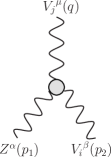
Figure 1: Vertex function $ie$ $\Gamma_{ZV_{i}V_{j}}^{\alpha\beta\mu}(p_{1},p_{2},q)$ for the $ZV_{i}V_{j}$ ($V_{i,j}=Z$, $\gamma$) couplings. All the four-momenta are outgoing.

In the next section we will consider a SM extension including complex nondiagonal couplings in the charged scalar sector. We will show that only the CP-odd form factors are induced by this mechanism.

III $ZZ^{*}\gamma$ and $ZZV^{*}$ CP-odd form factors

We consider a renormalizable effective theory with several physical charged scalars bosons. We will assume that there are trilinear vertices $\Phi_{i}\Phi_{j}V$, which can induce TNGBCs at the one-loop level via triangle diagrams. The Lagrangian describing such trilinear interactions between the neutral gauge bosons and the charged scalar bosons can be written as ${\mathcal{L}}={\mathcal{L}}_{D}+{\mathcal{L}}_{ND}$, where ${\mathcal{L}}_{D}$ describes the diagonal couplings and ${\mathcal{L}}_{ND}$ the nondiagonal ones. The gauge invariant structure of these Lagrangians is as follows

$${\mathcal{L}}_{D} = ie\sum_{i}Q_{\Phi}A_{\mu}\Phi_{i}^{+}\overleftrightarrow{\partial}^{\mu}\Phi_{i}^{-}+ig\sum_{i}g_{ii}^{Z}Z_{\mu}\Phi_{i}^{+}\overleftrightarrow{\partial}^{\mu}\Phi_{i}^{-},$$ (5)

$${\mathcal{L}}_{ND} = i\sum_{i\neq j}g_{ij}^{Z}Z_{\mu}\Phi_{i}^{+}\overleftrightarrow{\partial}^{\mu}\Phi_{j}^{-}+\text{H.c}.$$ (6)

where the coupling constants $g_{ii}^{Z}$ are real due to the Lagrangian hermicity, whereas $g_{ij}^{Z}$ could be complex. From here we extract the Feynman rules for the interaction between neutral gauge bosons and the charged scalars bosons, $V_{\mu}\Phi_{i}^{+}(k_{1})\Phi_{j}^{-}(k_{2})$, which has the generic form $ieg_{ij}^{V}(k_{1}-k_{2})_{\mu}$, where all the four-momenta are outgoing. For $V=\gamma$, there are only diagonal couplings and $g_{ii}^{\gamma}=Q_{\Phi}$ is the charge of the scalar boson in units of $e$.

It is worth mentioning that in the class of theories we are considering, quartic vertices of the kind $V_{i}^{\alpha}V_{j}^{\beta}\Phi_{i}^{\pm}\Phi_{j}^{\mp}$ would also appear. In principle, this class of vertices can contribute to TNGBCs at the one-loop level through bubble diagrams such as the one depicted in Figure 2. However since the renormalizable quartic vertex would be proportional to the metric tensor $g^{\alpha\beta}$, the amplitude arising from this of diagram can be written as

$${\cal M}^{\alpha\beta\mu}_{bubble}\sim\int\frac{d^{D}k}{(2\pi)^{D}}\frac{(2k+q)^{\mu}g^{\alpha\beta}}{(k^{2}-m_{i}^{2})((k+q)^{2}-m_{j}^{2})}\sim g^{\alpha\beta}q^{\mu}.$$ (7)

Therefore this diagram does not contribute to our TNGBC form factors. All other possible diagrams obtained by permuting the $Z$ gauge bosons contribute with terms that can be dropped when the transversality condition for the on-shell gauge bosons are taken into account and also when considering that the virtual gauge boson is attached to a conserved current.

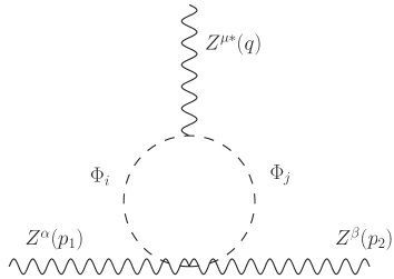
Figure 2: Illustrative bubble diagram arising from the quartic vertex $ZZ\Phi_{i}^{\pm}\Phi_{j}^{\mp}$, which can appear in the class of theories we are interested in. Since this vertex is proportional to the metric tensor $g^{\alpha\beta}$, the amplitude of this diagram is proportional to $q^{\mu}$ and does not contribute to our CP-violating TNGBC form factors, which neither receive contributions from all other bubble diagrams obtained by exchanging the $Z$ gauge bosons.

We now present our results for the one-loop contributions to the $ZV^{*}\gamma$ and $ZZV^{*}$ couplings, where $V^{*}$ stands for an off-shell gauge boson. Since only the $Z$ gauge boson has nondiagonal $Z\Phi_{i}^{\pm}\Phi_{j}^{\mp}$ couplings, the $Z\gamma^{*}\gamma$ form factor will not be induced at the one-loop level via this mechanism. Also, no CP-even form factor is induced via scalar couplings since the Levi-Civitta tensor cannot be generated this way. We will set $Q_{\Phi}=-1$, but the results will also be valid for the contribution of a pair of doubly charged scalar bosons, though in this case there will be an additional proportionality factor of $2$ appearing in the $ZZ^{*}\gamma$ and $ZZ\gamma^{*}$ vertices. Once the amplitude for each Feynman diagram was written down, the Passarino-Veltman method was applied to obtain scalar integrals, which are suitable for numerical evaluation.

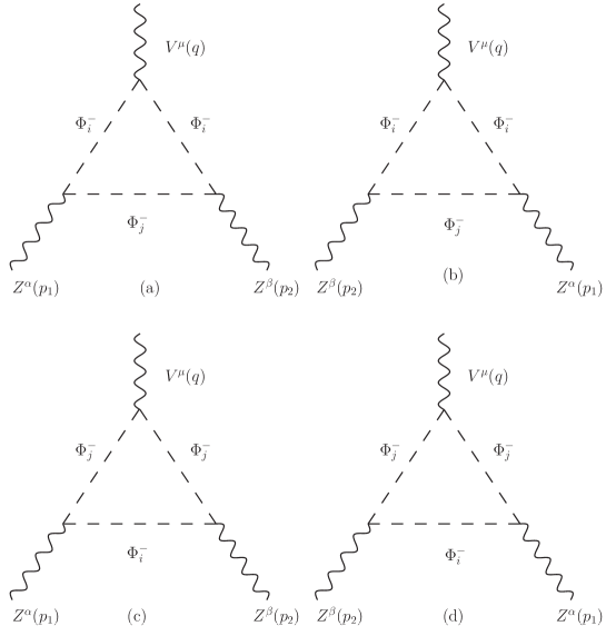
Figure 3: One-loop level Feynman diagrams inducing the $ZZ^{*}\gamma$ ($V=\gamma$ ) coupling.

III.1 $ZZ^{*}\gamma$ coupling

The Feynman diagrams contributing to the $Z_{\alpha}(p_{1})Z_{\beta}^{*}(p_{2})\gamma_{\mu}(q)$ coupling are shown in Figure 3. It is interesting to note that diagram (b) is required by Bose symmetry, whereas diagrams (c) and (d), which involve the exchange of the virtual scalars bosons, are necessary to cancel out ultraviolet divergences. After the mass-shell and transversality conditions for the gauge bosons are considered, we obtain the following results

$$h_{1}^{Z}(p_{2}^{2},m_{i}^{2},m_{j}^{2}) = \frac{m_{Z}^{2}\text{Im}\left(g_{ij}^{Z}{g_{ji}^{Z}}^{*}\right)}{6\pi^{2}(m_{Z}^{2}-p_{2}^{2})^{3}}\Big{\{}2m_{i}^{2}\left(p_{2}^{2}-m_{Z}^{2}\right)B_{ii}(0)+3m_{j}^{2}(m_{Z}^{2}-p_{2}^{2})\left(m_{i}^{2}-m_{j}^{2}-m_{Z}^{2}\right)C_{ijj}(p_{2}^{2})$$ (8)

$$- \frac{1}{2}(m_{i}^{2}-m_{j}^{2})\left((m_{Z}^{2}-p_{2}^{2})(B_{ij}(0)-1)+3(m_{Z}^{2}+p_{2}^{2})B_{ij}(p_{2}^{2})-6m_{Z}^{2}B_{ij}(m_{Z}^{2})\right)-\left(i\leftrightarrow j\right)\Big{\}},$$

$$h_{2}^{Z}(p_{2}^{2},m_{i}^{2},m_{j}^{2}) = \frac{m_{Z}^{4}\text{Im}\left(g_{ij}^{Z}{g_{ji}^{Z}}^{*}\right)}{6\pi^{2}(m_{Z}^{2}-p_{2}^{2})^{4}}\Big{\{}4m_{i}^{2}\left(p_{2}^{2}-m_{Z}^{2}\right)B_{ii}(0)-3m_{j}^{2}(m_{Z}^{2}-p_{2}^{2})\left(m_{Z}^{2}+p_{2}^{2}-2(m_{i}^{2}-m_{j}^{2})\right)C_{ijj}(p_{2}^{2})$$

$$- \frac{1}{2}(m_{i}^{2}-m_{j}^{2})\left(2(m_{Z}^{2}-p_{2}^{2})(B_{ij}(0)-1)+3(m_{Z}^{2}+3p_{2}^{2})B_{ij}(p_{2}^{2})-3(3m_{Z}^{2}+p_{2}^{2})B_{ij}(m_{Z}^{2})\right)-\left(i\leftrightarrow j\right)\Big{\}}$$

where $p_{2}$ is the four-momentum of the off-shell $Z$ gauge boson, $m_{i,j}$ stand for the masses of the charged scalar bosons and the coefficient $2i\text{Im}(g_{ij}^{Z}{g_{ji}^{Z}}^{*})=g_{ij}^{Z}{g_{ji}^{Z}}^{*}-{g_{ij}^{Z}}^{*}g_{ji}^{Z}$ contains the imaginary phase that induces CP violation, which is necessary to obtain nonzero results and is consistent with the Lorentz structure of the Lagrangian. We also have introduced the shorthand notation $B_{ab}(c^{2})=B_{0}(c^{2},m_{a}^{2},m_{b}^{2})$, $C_{abc}(p_{2}^{2})=C_{0}(m_{Z}^{2},0,p_{2}^{2},m_{a}^{2},m_{b}^{2},m_{c}^{2})$ and $C_{abc}(q^{2})=C_{0}(m_{Z}^{2},m_{Z}^{2},q^{2},m_{a}^{2},m_{b}^{2},m_{c}^{2})$, where $B_{0}$ and $C_{0}$ stand for Passarino-Veltman scalar functions. From the above expressions, it is evident that the form factors vanish when the masses of the charged scalar bosons are degenerate. It is also straightforward to show that ultraviolet divergences cancel out.

III.2 $ZZ\gamma^{*}$ coupling

The Feynman diagrams for the $Z_{\alpha}(p_{1})Z_{\beta}(p_{2})\gamma_{\mu}^{*}(q)$ couplings are similar to those inducing the $ZZ^{*}\gamma$ coupling, but in this case the photon is off-shell. The corresponding form factor is given by:

$$f_{4}^{\gamma}(q^{2},m_{i}^{2},m_{j}^{2}) = \frac{m_{Z}^{2}\text{Im}\left(g_{ij}^{Z}{g_{ji}^{Z}}^{*}\right)}{12m_{Z}^{2}\pi^{2}q^{2}(4m_{Z}^{2}-q^{2})^{2}}\Big{\{}(m_{i}^{2}-m_{j}^{2})\left(12m_{Z}^{2}B_{ij}(m_{Z}^{2})+(4m_{Z}^{2}-q^{2})(1-B_{ij}(0))\right)$$ (10)

$$+ \left(q^{2}\left(m_{i}^{2}+3m_{j}^{2}+7m_{Z}^{2}-q^{2}\right)+6\left(m_{i}^{2}-m_{j}^{2}\right)^{2}-2m_{Z}^{2}(8m_{i}^{2}-3m_{Z}^{2})\right)B_{ii}(q^{2})$$

$$- 6\left(m_{i}^{2}-m_{j}^{2}-m_{Z}^{2}\right)\left(m_{i}^{4}-2m_{i}^{2}\left(m_{j}^{2}+m_{Z}^{2}\right)+\left(m_{j}^{2}-m_{Z}^{2}\right)^{2}+m_{j}^{2}q^{2}\right)C_{iji}(q^{2})-(i\leftrightarrow j)\Big{\}},$$

where $q$ is the photon four-momentum. As expected, this form factor is proportional to $\text{Im}(g_{ij}^{Z}{g_{ji}^{Z}}^{*})$ and vanishes when $m_{i}=m_{j}$.

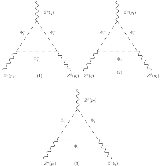
Figure 4: Generic one-loop Feynman diagrams for the $ZZZ^{*}$ coupling. The complete set of diagrams is obtained by permuting $Z_{\alpha}(p_{1})$ and $Z_{\beta}(p_{2})$ and exchanging the charged scalars bosons.

III.3 $ZZZ^{*}$ coupling

Because of Bose symmetry, in the case of the $ZZZ^{*}$ coupling, there are several more diagrams than those inducing the $ZZ^{*}\gamma$ vertex. We present in Figure 4 the generic Feynman diagrams from which all diagrams inducing the $ZZZ^{*}$ vertex can be generated. Notice that diagrams (2) and (3) are obtained from diagram (1) after performing the permutations $Z_{\alpha}(p_{1})\leftrightarrow Z_{\mu}(q)$, and $Z_{\beta}(p_{2})\leftrightarrow Z_{\mu}(q)$, respectively. Additional diagrams are obtained from these diagrams following a similar procedure as that described in Fig. 3: for each one of the Feynman diagrams of Fig. 4 there are three more diagrams that are obtained similarly as diagrams (b)-(d) of Fig. 3, which are obtained from diagram (a) by permuting the $Z$ gauge bosons and exchanging the charged scalars. Therefore, there are a total of twelve Feynman diagrams for the $ZZZ^{*}$ coupling. By using the appropriate simplifications, the amplitude of each diagram of Figure 4 reduces to those of the $ZZ^{*}\gamma$ and $ZZ\gamma^{*}$ couplings. The diagrams (2) and (3) of Fig. 4 not only are required by Bose symmetry but, once their amplitudes are added up, ultraviolet divergences cancel out. After the Passarino-Veltman method is applied, we obtain the following result

$$f_{4}^{Z}(q^{2},m_{i}^{2},m_{j}^{2}) = \frac{m_{Z}^{2}g_{ii}^{Z}\text{Im}\left(g_{ij}^{Z}{g_{ji}^{Z}}^{*}\right)}{12\pi^{2}s_{W}q^{2}(q^{2}-m_{Z}^{2})(q^{2}-4m_{Z}^{2})^{2}}$$ (11)

$$\times \Big{\{}q^{2}\left(q^{2}\left(m_{i}^{2}+3m_{j}^{2}+7m_{Z}^{2}\right)+6\left(m_{i}^{2}-m_{j}^{2}\right)^{2}-16m_{i}^{2}m_{Z}^{2}-6m_{Z}^{4}-q^{4}\right)B_{ii}(q^{2})$$

$$+ \left(m_{Z}^{2}q^{2}\left(10m_{Z}^{2}-13m_{i}^{2}-3m_{j}^{2}\right)+6m_{Z}^{2}(m_{i}^{2}-m_{j}^{2})\left(m_{i}^{2}-m_{j}^{2}+2m_{Z}^{2}\right)+q^{4}\left(4m_{i}^{2}-m_{Z}^{2}\right)\right)B_{ii}(m_{Z}^{2})$$

$$- (m_{i}^{2}-m_{j}^{2})\left(2q^{2}\left(4m_{Z}^{2}-q^{2}\right)(1-B_{ij}(0))-3q^{4}B_{ij}(q^{2})-3m_{Z}^{2}\left(4m_{Z}^{2}-7q^{2}\right)B_{ij}(m_{Z}^{2})\right)$$

$$- 6\left(m_{i}^{2}-m_{j}^{2}+2m_{Z}^{2}\right)\left(m_{Z}^{2}q^{2}\left(m_{Z}^{2}-3m_{i}^{2}-m_{j}^{2}\right)+m_{Z}^{2}\left(m_{i}^{2}-m_{j}^{2}\right)^{2}+m_{i}^{2}q^{4}\right)C_{iij}(q^{2})$$

$$- 6q^{2}\left(m_{i}^{2}-m_{j}^{2}-m_{Z}^{2}\right)\left(m_{i}^{4}-2m_{i}^{2}\left(m_{j}^{2}+m_{Z}^{2}\right)+\left(m_{j}^{2}-m_{Z}^{2}\right)^{2}+m_{j}^{2}q^{2}\right)C_{iji}(q^{2})-(i\leftrightarrow j)\Big{\}},$$

where $q$ is now the four-momentum of the off-shell $Z$ boson. We note that all the properties discussed above are also present in this form factor. In the next section we will evaluate the CP-violating TNGBCs for illustrative values of the charged scalar boson masses and the four-momentum of the virtual gauge boson.

IV Numerical results and discussion

While the diagonal couplings $V\Phi_{i}^{\pm}\Phi_{i}^{\mp}$ can appear in several extensions of the SM at the tree-level, the presence of the nondiagonal couplings $Z\Phi_{i}^{\pm}\Phi_{j}^{\mp}$ is less common, but they can be induced indeed within a more general renormalizable theory. In order to analyze the CP violating TNGBC form factors, we will not consider specific values for $g_{ii}^{Z}$ nor $\text{Im}(g_{ij}^{Z}{g_{ji}^{Z}}^{*})$. Therefore, the masses of the charged scalar bosons $m_{i,j}$ and the four-momentum of the virtual gauge boson will be the only free parameters involved in our analysis.

A particle with the properties of the SM Higgs boson with a mass of 125 GeV has been finally discovered at the LHC Aad et al. (2012b); Chatrchyan et al. (2012a), and the search for singly ($\Phi^{+}$) and doubly charged ($\Phi^{++}$) scalar bosons is still underway by the ATLAS Aad et al. (2013b, c, 2012c, 2012d) and CMS Chatrchyan et al. (2012b, c) collaborations. However, no evidence for the existence of such scalars bosons has been found up to date. Based on data collected in 2011, the ATLAS collaboration performed a model independent analysis to search for a light charged Higgs boson with a mass in the range 90-160 GeV Aad et al. (2013b). Independently, the CMS collaboration reported a search for the charged Higgs boson of the MSSM with a mass ranging from 80 to 160 GeV Chatrchyan et al. (2012b). This collaboration also reported a lower bound on the doubly charged Higgs boson mass between 204 and 449 GeV from the processes $pp\to\Phi^{++}\Phi^{--}\to\ell_{\alpha}^{+}\ell_{\beta}^{+}\ell_{\gamma}^{-}\ell_{\delta}^{-}$, and $pp\to\Phi^{++}\Phi^{-}\to\ell_{\alpha}^{+}\ell_{\beta}^{+}\ell_{\gamma}^{-}\nu_{\delta}$ Chatrchyan et al. (2012c). Such an analysis was done in the context of the minimal type II seesaw model and the singly and doubly charged scalar bosons were taken to be mass degenerate.

In the following analysis, we will consider that there is a charged scalar boson with a mass $m_{i}$ above 300 GeV, which is consistent with measurement of the ATLAS and CMS collaborations. Since the form factors depend on the splitting between the masses of the charged scalar bosons $\Delta m_{ij}=m_{j}-m_{i}$, we will use the parameters $m_{i}$ and $\Delta m_{ij}$ in our analysis below, along with the magnitude of the four-momentum of the virtual gauge boson, which we denote generically as $||p||$. The region of interest corresponds to $\Delta m_{ij}>0$ but for completeness we will also analyze the region $-m_{i}\leq\Delta m_{ij}\leq 0$, namely, the scenario with $m_{j}\leq m_{i}$. Such a region, which corresponds to a very light charged scalar boson, is not favored by experimental data, but we will consider it in our analysis in order to show the consistency of our results. We will thus analyze the behavior of the form factors as functions of $||p||$ and $\Delta m_{ij}$ for three illustrative values of $m_{i}$. We will show that all the form factors can have both real and imaginary parts. The latter appears when the magnitude of $||p||$ reaches the value of the sum of the masses of the charged scalar bosons to which the virtual gauge boson is attached and it is a reflect of the fact that a pair of real charged scalars could be produced at a collider, rather than two virtual ones, via an off-shell gauge boson.

IV.1 The form factor $h_{1}^{Z}$

To begin with, we show in Figure 5 the real (top plots) and imaginary (bottom plots) parts of the $h_{1}^{Z}$ form factor as functions of the four-momentum magnitude $||p_{2}||$ (left plots) and the splitting of the charged scalar boson masses $\Delta m_{ij}$ (right plots). For best appreciation of the curves we show the absolute value of the real and imaginary parts of the form factor. We use three distinct values of $m_{i}$: $300$, $400$ and $500$ GeV.

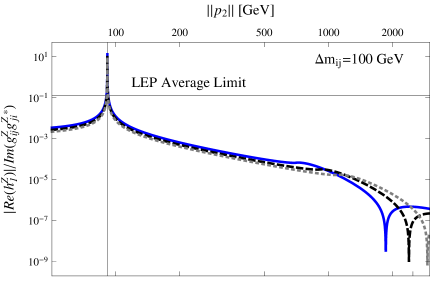
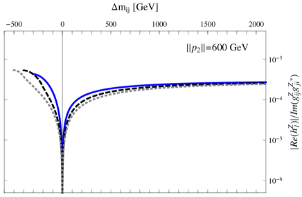
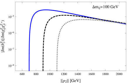
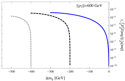
Figure 5: Behavior of the real (top plots) and imaginary (bottom plots) parts of the $h_{1}^{Z}$ form factor as functions of the four-momentum magnitude $||p_{2}||$ of the virtual $Z$ gauge boson (left plots) and the splitting of the charged scalar boson masses $\Delta m_{ij}=m_{j}-m_{i}$ (right plots). We use the indicated values of $\Delta m_{ij}$ and $||p_{2}||$ and each curve correspond to a distinct value of the charged scalar mass $m_{i}$: $m_{i}=300$ GeV (solid line), $400$ GeV (dashed line), and $500$ GeV (dotted line). The horizontal line in the top-left plot corresponds to the average value of the LEP lower and upper limits Achard et al. (2004). We note that the curves stop because $m_{j}=0$ is reached.

We will first analyze the behavior of the real part of the $h_{1}^{Z}$ form factor (top plots). It can be observed in Eq. (8) that $h_{1}^{Z}$ includes the term $m_{Z}^{2}-p_{2}^{2}$ in the denominator and thus it becomes undefined when $p_{2}^{2}\to m_{Z}^{2}$, which explains the sharp peak at $||p_{2}||=m_{Z}$ in the top-left plot, where we include a vertical line for illustrative purposes. This effect is not in conflict with Landau-Yang’s theorem since the full vertex function (3) does vanish when all the $Z$ gauge bosons are taken on-shell. In the $||p_{2}||>1600$ GeV region of the top-left plot a dip appears in each curve, though in the plot it is only visible in the $m_{i}=300$ GeV curve. This is due to a flip of sign of $h_{1}^{Z}$: in the $||p_{2}||<m_{Z}$ region the $h_{1}^{Z}$ form factor is positive, whereas in the $||p_{2}||>m_{Z}$ region it is negative and changes sign again in the dip located at $||p_{2}||>1600$. It is also interesting to note that the largest values of the real part of $h_{1}^{Z}$ are reached around $||p_{2}||\sim m_{Z}$. For instance, in units of $\text{Im}(g_{ij}^{Z}{g_{ji}^{Z}}^{*})$, we have $|h_{1}^{Z}|\sim 10^{-3}$ for $||p_{2}||\simeq 100$ GeV and $|h_{1}^{Z}|\sim 10^{-5}$ for $||p_{2}||=1000$ GeV. This is to be compared with the average value obtained from the LEP lower and upper bounds on the $h_{1}^{Z}$ form factor Achard et al. (2004) (horizontal line of the top-left plot). As far as the behavior of $h_{1}^{Z}$ as a function of $\Delta m_{ij}$ is concerned, while the region with large $\Delta m_{ij}$ corresponds to a heavy $m_{j}$, the $-m_{i}\leq\Delta m_{ij}\leq 0$ region corresponds to the scenario with a very light charged scalar boson with a mass lying in the interval $0\leq m_{j}\leq m_{i}$. Although this scenario seems to be ruled out by experimental data, we include it in our analysis for completeness. We note that in these and subsequent plots the stop of the curves is due to the reach of $m_{j}=0$. As expected, since degenerate charged scalar bosons do not give rise to CP-violating form factors, the form factors vanish when $\Delta m_{ij}=0$, this is why in the top-right plot we observe a sharp dip at $\Delta m_{ij}=0$, which is due to the vanishing of the form factor. We also note that the real part of the $h_{1}^{Z}$ form factor is not sensitive to a change in the splitting $\Delta m_{ij}$, so the different curves are almost indistinguishable.

As far as the imaginary part of $h_{1}^{Z}$ is concerned, which we show in the bottom plots of Fig. 5, since the photon must couple to the same charged scalar boson circulating into the loop, the $Z$ gauge boson must necessarily couple to distinct charged scalar bosons. Thus the imaginary part of $h_{1}^{Z}$ can only appear when $||p_{2}||\geq m_{i}+m_{j}$, which is evident in the curves of the bottom-left plot. It means that a higher energy would be required to measure such imaginary part unless there was a relatively light charged scalar, which is a scenario ruled out by experimental data. On the other hand, when the value of $||p_{2}||$ is fixed the imaginary part of $h_{1}^{Z}$ can only appear in the small region $0\leq m_{j}\leq||p_{2}||-m_{i}$ or $-m_{i}\leq\Delta m_{ij}\leq||p_{2}||-2m_{i}$, as shown in the bottom-right plot. This interval becomes narrower for increasing $m_{i}$: for instance when $||p_{2}||=600$ GeV, the imaginary part of $h_{1}^{Z}$ is nonvanishing in the interval $0\leq m_{j}\leq 300$ GeV for $m_{i}=300$ GeV, $0\leq m_{j}\leq 200$ GeV for $m_{i}=400$ GeV and $0\leq m_{j}\leq 100$ GeV for $m_{i}=500$ GeV. Again, we only include these results in our analysis for completeness. In general terms, we observe that the imaginary part of the $h_{1}^{Z}$ form factor can have a size of similar order of magnitude than its real part, in the same interval of the region of parameters where the former is nonvanishing. However the maximal size of the imaginary part is reached for a very light charged scalar, whereas the maximal size of the real part can be reached around the $Z$ resonance, where there is no imaginary part.

IV.2 The form factor $h_{2}^{Z}$

We now present in Figure 6 the corresponding plots for the $h_{2}^{Z}$ form factor, namely, we show the behavior of the real (top plots) and imaginary (bottom plots) parts of the form factor $h_{2}^{Z}$ as functions of $||p_{2}||$ (left plots) and $\Delta m_{ij}$ (right plots). We use the same set of parameters as in Fig. 5. We note that in general the $h_{2}^{Z}$ form factor shows a similar behavior to that of the $h_{1}^{Z}$ form factor, though there are some slight differences. We first analyze the top plots of Fig. 6, which show the real part of $h_{2}^{Z}$. We observe that apart from the sharp peak at $||p_{2}||=m_{Z}$ in the top-left plot, there are also dips at high energy, such as occurs in the respective $h_{1}^{Z}$ curves. Such dips, which are a result of the flip of sign of the form factor, are now shifted to the left and they appear at a higher $||p_{2}||$ for a smaller $m_{i}$, which is opposite to the behavior of $h_{1}^{Z}$. Thus the dip for $m_{i}=300$ GeV curve is not shown in the plot. In the $||p_{2}||<m_{Z}$ region $h_{2}^{Z}$ is negative, whereas in the $||p_{2}||>m_{Z}$ region it is positive, contrary to what happens with $h_{1}^{Z}$. After the dip at $||p_{2}||\geq 1000$ GeV, $h_{2}^{Z}$ becomes negative again. We also note that the magnitude of $h_{1}^{Z}$ is greater than that of $h_{2}^{Z}$, although for very high values of $||p_{2}||$ or very heavy $m_{i}$, the both $h_{1}^{Z}$ and $h_{2}^{Z}$ are considerably suppressed. As expected, the largest values of the real part of $h_{2}^{Z}$ are reached around $||p_{2}||\sim m_{Z}$. For instance, in units of $\text{Im}(g_{ij}^{Z}{g_{ji}^{Z}}^{*})$, we have $|h_{2}^{Z}|\sim 10^{-6}$ for $||p_{2}||=100$ GeV and $|h_{2}^{Z}|\sim 10^{-7}$ for $||p_{2}||=1000$ GeV. It can also be observed that, $h_{2}^{Z}$ is more sensitive than $h_{1}^{Z}$ to a change in the value of $m_{i}$. Regarding the top-right plot, again we observe that the $h_{2}^{Z}$ form factor vanishes when $m_{i}=m_{j}$, which shows the consistency of our result. The curves of the top-right plot show a dip in the $-m_{i}\leq\Delta m_{ij}\leq 0$ region , which are due to a change of sign and do not appear in the case of the $h_{1}^{Z}$ form factor. Although $h_{2}^{Z}$ can reach its largest values in this region, as explained above, it corresponds to the case of a very light charged scalar.

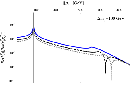
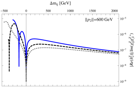
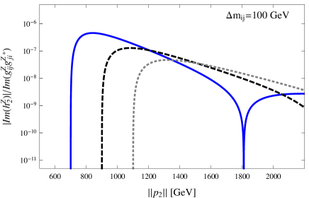
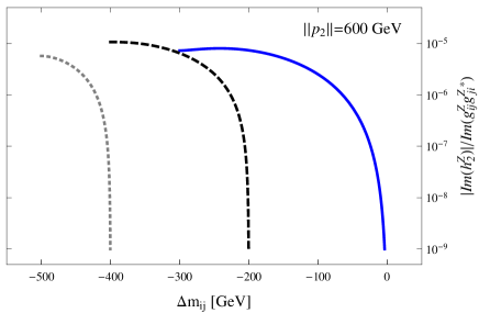
Figure 6: The same as in Fig. 5, but for the $h_{2}^{Z}$ form factor.

As in the case of $h_{1}^{Z}$ (both $h_{1}^{2}$ and $h_{2}^{Z}$ form factors arise from the same vertex function), the imaginary part of $h_{2}^{Z}$ would be nonvanishing when $||p_{2}||\geq m_{i}+m_{j}$, which again is evident in the bottom-left plot of Figure 6. Therefore, to observe such an imaginary part a higher energy than that required to observe the respective real part would be required. Furthermore, although the sizes of the imaginary part and the real part are similar, the real part can reach larger values in the interval where the imaginary part vanishes. Thus, in general the imaginary part is smaller than the largest possible values of the real part, which is reached around the $Z$ resonance. As far as the behavior of the imaginary part of $h_{2}^{Z}$ as a function of $\Delta m_{ij}$ is concerned, as expected it is nonvanishing in the interval $-m_{i}\leq\Delta m_{ij}\leq||p_{2}||-2m_{i}$, where $m_{j}$ is very light. In this region the imaginary part of $h_{2}^{Z}$ can reach values slightly larger than the real part.

IV.3 The form factor $f_{4}^{\gamma}$

We now turn to analyze the $f_{4}^{\gamma}$ form factor. We note that it becomes undefined when $||q||\to 0$ as can be inferred from Eq. (10). Nevertheless, Landau-Yang’s theorem is obeyed as can be deduced after a closer inspection of Eq. (4). In the top plots of Figure 7 we show the real part of $f_{4}^{\gamma}$ as a function of the four-momentum magnitude $||q||$ (left plot) and the mass splitting $\Delta m_{ij}$ (right plot). On the other hand, similar plots are shown in the bottom part of the panel that illustrate the behavior of the imaginary part of $f_{4}^{\gamma}$. In this analysis we will use the same set of $m_{i}$ values used in Fig. 5.

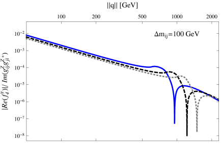
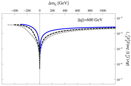
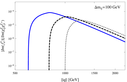
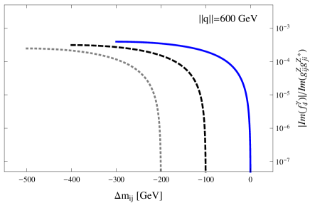
Figure 7: Behavior of the real (top plots) and imaginary (bottom plots) parts of the $f_{4}^{\gamma}$ form factor as a function of the four-momentum magnitude $||q||$of the virtual photon (left plots) and the splitting of the charged scalar boson masses $\Delta m_{ij}$ (right plots). We use the indicated values for $\Delta m_{ij}$ and $||q||$ and each curve correspond to a distinct value of the charged scalar mass $m_{i}$: $m_{i}=300$ GeV (solid line), $400$ GeV (dashed line), and $500$ GeV (dotted line). As explained in the text, the imaginary part of $f_{4}^{\gamma}$ arises only when $||q||\geq 2m_{i}$ in the bottom-left plot and $0\leq m_{j}\leq\frac{||q||}{2}$ or $-m_{i}\leq\Delta m_{ij}\leq\frac{||q||}{2}-m_{i}$ in the bottom-right plot.

As far as the real part of the $f_{4}^{\gamma}$ form factor is concerned, we note that the dip appearing in each curve of the top-left plot corresponds to a flip of sign of $f_{4}^{\gamma}$, which turns from negative to positive at $||q||\simeq$ 950, 1100, and 1500 GeV for $m_{i}=$300, 400, and 500 GeV, respectively. We also observe that this form factor decouples at high energy, where it has a negligible magnitude, but in the interval between $100$ GeV and 900 GeV it can reach values as higher as $10^{-5}-10^{-3}$, in units of $\text{Im}(g_{ij}^{Z}{g_{ji}^{Z}}^{*})$. It is also interesting to note that the real part of $f_{4}^{\gamma}$ is not very sensitive to a variation of the charged scalar mass $m_{i}$, which contrasts with the behavior of the imaginary part. On the other hand, in the top-right plot of Figure 7, we show the behavior of $f_{4}^{\gamma}$ as a function of $\Delta m_{ij}$ for $||q||=600$ GeV and the same three values of $m_{i}$ used in previous analyses. We observe that the magnitude of $f_{4}^{\gamma}$ does not increase significantly as $\Delta m_{ij}$ increases. As expected, this form factor vanishes when $\Delta m_{ij}=0$. We note that the maximal values of the real part of $f_{4}^{\gamma}$ are of the order of $10^{-3}-10^{-2}$ times the factor $\text{Im}(g_{ij}^{Z}{g_{ji}^{Z}}^{*})$.

In the bottom plots of Figure 7 we show the behavior of the imaginary part of $f_{4}^{\gamma}$. Since the virtual photon must necessarily couple to the same charged scalar boson, the imaginary part of this form factor would arise when $||q||\geq\min\left(2m_{i},2m_{j}\right)$, which is evident in the bottom-right plot, where the imaginary part is nonzero for $||q||\geq 2m_{i}$. For fixed $m_{i}$, the interval for nonvanishing imaginary part can be written as $-m_{i}\leq\Delta m_{ij}\leq\frac{||q||}{2}-m_{i}$ or $0\leq m_{j}\leq\frac{||q||}{2}$. This is the reason why the curves in the bottom-right plot are nonvanishing only in the small region where $-300$ GeV $\leq\Delta m_{ij}\leq 0$ GeV for $m_{i}=300$ GeV, $-400$ GeV $\leq\Delta m_{ij}\leq-100$ GeV for $m_{i}=400$ GeV and $-500$ GeV $\leq\Delta m_{ij}\leq-200$ GeV for $m_{i}=500$ GeV. Again we note that the imaginary part of $f_{4}^{\gamma}$ has a similar order of magnitude than its real part, namely $10^{-5}$ times $\text{Im}(g_{ij}^{Z}{g_{ji}^{Z}}^{*})$. However, as in the previous form factors, the real part can reach larger values in the region where the imaginary part vanishes than in the region where both of them are nonzero.

IV.4 The form factor $f_{4}^{Z}$

Finally we show in Figure 8 the real (top plots) and imaginary (bottom plots) parts of the form factor $f_{4}^{Z}$ as a function of the four-momentum magnitude $||q||$ (left plots) and the mass splitting $\Delta m_{ij}$ (right plots). We consider the same scenarios analyzed above.

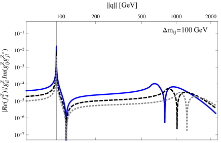
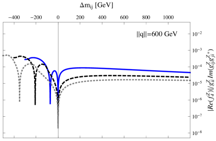
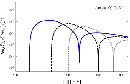
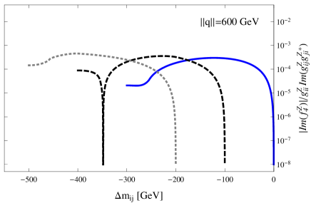
Figure 8: The same as in Fig. 7 but for the $f_{4}^{Z}$ form factor. Unlike the $f_{4}^{\gamma}$ form factor, which becomes undefined in $||q||=0$, the $f_{4}^{Z}$ form factor gets undefined in $||q||=m_{Z}$.

We first analyze the behavior of the real part of $f_{4}^{Z}$ (top plots) as a function of $||q||$ and $\Delta m_{ij}$. This form factor has a sharp peak at $||q||=m_{Z}$ due to the factor $q^{2}-m_{Z}^{2}$ in the denominator. There are also two dips appearing in the curves of the top-left plot, which as in the previous cases are due to a sign flip of this form factor. We observe that, unlike the $h_{1,2}^{Z}$ form factors, $f_{4}^{Z}$ flips sign twice for $m_{Z}\leq||q||\leq 2000$ GeV. One of such sign flips occurs at $||q||\simeq 110$ GeV, regardless of the $m_{i}$ value, and the second flip occurs at $||q||\simeq 800$, 1000, and 1250 GeV for $m_{i}=300$, 400, and 500 GeV, respectively. Inside the region enclosed by the two dips the real part of $f_{4}^{Z}$ is positive, and it is negative outside this region. Although the larger values of $f_{1}^{Z}$ are reached around the $Z$ resonance, there is an increase of the real part of $f_{4}^{Z}$ in the interval between $||q||=$140 GeV and $||q||=$700 GeV, where the real part of $f_{4}^{Z}$ goes from $10^{-6}$ up to $10^{-5}$, in units of $g_{ii}^{Z}\text{Im}(g_{ij}^{Z}{g_{ji}^{Z}}^{*})$.

The $f_{4}^{Z}$ for factor develops an imaginary part when $||q||\geq\min\left(2m_{i},m_{i}+m_{j},2m_{j}\right)$ since in this loop the virtual $Z$ boson can now couple to the same or distinct charged scalar bosons. In the bottom-left plot we have $m_{j}>m_{i}$, thus the imaginary part of $f_{4}^{Z}$ arises when $||q||\geq 2m_{i}$. On the other hand, for the chosen values of $m_{i}$, in the left plot we have $m_{i}\geq\frac{||q||}{2}$, thus the interval where the imaginary part of $f_{4}^{Z}$ is nonzero is given by $||q||\geq 2m_{j}$ or in terms of the mass-splitting $-m_{i}\leq\Delta m_{ij}\leq\frac{||q||}{2}-m_{i}$, as observed in the curves shown in the bottom-right plot. Thus $f_{4}^{\gamma}$ and $f_{4}^{Z}$ develop imaginary parts in the same interval. Most part of this interval correspond to a very light charged scalar and as occurs with the other form factors, the imaginary part of $f_{4}^{Z}$ has a size of the same order of magnitude than its real part, which however can reach much higher values outside this region.

It is interesting to note that the $f_{4}^{Z}$ form factor was also studied in the framework of a THDM where the respective contribution is induced by three nondegenerate neutral scalar bosons Chang et al. (1995). In such a model three different nondiagonal complex couplings ${\mathcal{O}}_{1i}$ arise in the neutral scalar sector. It was reported in Chang et al. (1995) that $f_{4}^{Z}$ can reach values from $10^{-6}\times{\mathcal{O}}_{11}{\mathcal{O}}_{12}{\mathcal{O}}_{13}$ to $10^{-5}\times{\mathcal{O}}_{11}{\mathcal{O}}_{12}{\mathcal{O}}_{13}$, where the following set of values for the free parameters was used: $\sqrt{s}=||q||=200$ GeV, $M_{3}=250$ GeV, $M_{2}=150$ GeV, and 60 GeV $\leq M_{1}\leq$ 150 GeV, with $M_{i}$ the masses of the neutral scalar bosons. In this case the ${\mathcal{O}}_{11}{\mathcal{O}}_{12}{\mathcal{O}}_{13}$ factor could suppress considerably the THDM contribution to $f_{4}^{Z}$, just as happens with the contribution of our charged scalar bosons, which could be suppressed by the factor $g_{ii}^{Z}\text{Im}(g_{ij}^{Z}{g_{ji}^{Z}}^{*})$.

V Conclusions

We have presented an analysis of the one-loop contributions to the CP-violating form factors associated with the $ZZ^{*}\gamma$, $ZZ\gamma^{*}$ and $ZZZ^{*}$ couplings in the framework of an arbitrary effective model with at least two nondegenerate charged scalar bosons that couple nondiagonally to the $Z$ gauge boson. Such form factors are induced only when the nondiagonal coupling constants $g_{ij}^{Z}$ are complex and have an imaginary phase. Our analysis is independent of any specific value of the coupling constants, so our results are scaled by the coefficient $g_{ii}^{V}\text{Im}(g_{ij}^{Z}{g_{ji}^{Z}}^{*})$. We considered a charged scalar boson with mass above 300 GeV, which is consistent with experimental constraints, and analyze the behavior of the real and imaginary parts of the form factors as functions of the four-momentum of the virtual gauge boson $||p||$ or $||q||$ and the splitting of the masses of the charged scalar bosons $\Delta m_{ij}=m_{j}-m_{i}$. Although the region which is consistent with experimental data corresponds to $\Delta m_{ij}\geq 0$, for completeness we also include the results for $-m_{i}\leq\Delta m_{ij}\leq 0$, which corresponds to $m_{j}$ lighter than $m_{i}$ . As far as the orders of magnitude of the form factors are concerned, they are as follows in units of $g_{ii}^{V}\text{Im}(g_{ij}^{Z}{g_{ji}^{Z}}^{*})$: $|h_{1}^{Z}|\sim 10^{-5}-10^{-4}$, $|h_{2}^{Z}|\sim 10^{-7}-10^{-6}$, $|f_{4}^{\gamma}|\sim 10^{-5}-10^{-3}$ and $|f_{4}^{Z}|\sim 10^{-6}-10^{-5}$, for values of $||p||$ about a few hundreds of GeVs. When the magnitude of $||p||$ increases, the real part of the form factors decreases smoothly and decouple at high energy. Furthermore, it is not very sensitive to large values of $\Delta m_{ij}$. As for its imaginary part, for an intermediate value of $||p||$ it can arise in a small region of values of $m_{i}$ and $m_{j}$, which corresponds mainly to the scenario with a relatively light charged scalar. Such scenario is not favored by current constraints on the mass of a charged scalar boson. On the other hand, for heavy $m_{i}$ and $m_{j}$, the imaginary part of the form factors can only arise for large $||p||$. Therefore a higher energy would be required in order that the form factors could develop an imaginary part, which can have a magnitude similar to the corresponding real part, though the latter can reach larger values in the region where the former vanishes. We also find that, except for a proportionality factor, our results for the $f_{4}^{Z}$ form factor are of the same order of magnitude than the contributions arising in a THDM with three nondegenerate neutral scalar bosons that couple nondiagonally to the $Z$ gauge boson. It is worth noticing that our results are valid for the contribution of nondegenerate doubly charged scalar bosons, though in this case the form factors associated with the $ZZ^{*}\gamma$ and $ZZ\gamma^{*}$ couplings would get an additional factor of two.

Although the LHC was down temporarily, it has resumed their operations with a higher center of mass energy and a higher integrated luminosity. A significant improvement in the experimental limits of the TNGBCs is thus expected in the forthcoming years. Therefore it is necessary to examine any potential contribution to the respective form factors.