Kinetic models of immediate exchange

Abstract

We propose a novel kinetic exchange model differing from previous ones in two main aspects. First, the basic dynamics is modified in order to represent economies where immediate wealth exchanges are carried out, instead of reshufflings or uni-directional movements of wealth. Such dynamics produces wealth distributions that describe more faithfully real data at small values of wealth. Secondly, a general probabilistic trading criterion is introduced, so that two economic units can decide independently whether to trade or not depending on their profit. It is found that the type of the equilibrium wealth distribution is the same for a large class of trading criteria formulated in a symmetrical way with respect to the two interacting units. This establishes unexpected links between and provides a microscopic foundations of various kinetic exchange models in which the existence of a saving propensity is postulated. We also study the generalized heterogeneous version of the model in which units use different trading criteria and show that suitable sets of diversified parameter values with a moderate level of heterogeneity can reproduce realistic wealth distributions with a Pareto power law.

I Introduction

Kinetic exchange models provide a minimal description of wealth exchange between economic units (representing, e.g., individuals, families, or companies) in a way formally similar to that in which energy is transferred between molecules of a fluid due to collisions Patriarca2010b ; Patriarca2013a . Such models were introduced independently in different fields such as social sciences Angle1986a ; Angle1992a ; Angle2006a , economics Bennati1988a ; Bennati1988b ; Bennati1993a , and physics Dragulescu2000a ; Dragulescu2001a ; Dragulescu2001b ; Yakovenko2009a ; Chakraborti2000a ; Chakraborti2002a . John Angle Angle1986a ; Angle1992a originally introduced this type of models basing them on the surplus theory, with the goal of describing the origin of wealth inequalities. Compared with other agent-based models of financial markets Samanidou2007a , the structure of kinetic exchange models is extremely simple: they only describe wealth flows between economic units without considering (explicitly) other elements of a market dynamics. However, even so they predict quite realistic shapes of wealth distributions Chatterjee2005b .

In kinetic exchange models it is assumed that the total wealth of the system is conserved, following in turn from wealth conservation during each unit-unit interaction. The dynamics can be formulated through the following update rule at a generic time iteration $t$ defining the wealth exchange between two units $j$ and $k$ chosen randomly among the $N$ units of the system ($j,k=1,\dots,N$),

$$x_{j}^{{}^{\prime}}=x_{j}+\Delta x_{jk}\,,$$ (1)

$$x_{k}^{{}^{\prime}}=x_{k}-\Delta x_{jk}\,.$$

Here $x_{j}$ and $x_{k}$ ($x_{j}^{{}^{\prime}}$ and $x_{k}^{{}^{\prime}}$) are the wealths of the trading units $j$ and $k$ before (after) the exchange and $\Delta x_{jk}=-\Delta x_{kj}$ is the exchanged amount of wealth. Without loss of generality, in Eqs. (1) the plus (minus) sign has been chosen for $j$ ($k$); who wins or loses depends on the sign of $\Delta x_{jk}$. The conservation of the total wealth of the system leads to an equilibrium wealth distribution that coincides formally with the Gibbs energy distribution.

As discussed in Ref. Patriarca2010b , most of kinetic exchange models can be formulated in a unified way, where the amount of exchanged wealth in Eqs. (1) is expressed as

$$\Delta x_{jk}=\tilde{\omega}_{jk}\,x_{k}-\tilde{\omega}_{kj}\,x_{j}\,.$$ (2)

Here $\tilde{\omega}_{jk}$ and $\tilde{\omega}_{kj}$ are two suitable stochastic variables in $(0,1)$ to be extracted at each trade, representing the fractions of wealth of unit $k$ and $j$, respectively, involved in the trade.

Various aspects of kinetic exchange models have been criticized. A first objection concerns wealth conservation. Namely, it is pointed out that the assumption of a perfect conservation of wealth is incompatible with the fact that in real systems wealth is not conserved, a most relevant reason being the existence of production-consumption processes. In fact, kinetic exchange models can be interpreted as models with homogeneous production and consumption. To show this, one can use a modified form of a kinetic exchange model where production and consumption have been explicitly added to the dynamics. It is convenient to start from Eqs. (1) and (2) and write the total wealth variation of a generic unit $j$ during a time step $\delta t$, defined as the time interval corresponding to one Monte Carlo swap over all the units $k$ ($k\neq j$),

$$\frac{x_{j}^{\prime}-x_{j}}{\delta t}\approx\sum_{k(k\neq j)}[J_{jk}x_{k}-J_{kj}x_{j}]+(p-c)x_{j}\,.$$ (3)

Here the homogeneous production and consumption terms have been added, with production and consumption rates $p$ and $c$, respectively; $J_{jk}=\tilde{\omega}_{jk}/\delta t$ (and analogously for $J_{kj}$). In the continuous time limit, $(x_{j}^{\prime}-x_{j})/\delta t\approx dx_{j}(t)/dt$, one can introduce the auxiliary variables

$$X_{j}(t)=x_{j}(t)\exp\!\int\!dt[p(t)-c(t)]\,,$$ (4)

where a possible time dependence of $p$ and $c$ has been taken into account. Equations (3) written in the new variables $X_{j}$ do not contain anymore the production and consumptions terms and turn into the equations of the corresponding model without production and consumption, in which wealth conservation holds. However, this is not valid in the case of strong heterogeneity, in which the consumption and production processes of each unit have to be taken into account separately.

Another critic toward kinetic exchange models claims that the type of trade dynamics they model can hardly resemble an actual economic trade. In fact, traditional approaches of economics assume that the decisions to carry out a trade are taken by rational agents or by economic agents with bounded rationality on the base of the total or partial information available about the system. Instead, kinetic exchange models may resemble at first sight more a hazard game, due to their random dynamics Hayes2002a ; Lux2005a . It is clear that due to their statistical nature kinetic exchange models certainly do not provide a direct picture of the economic trading or the exchange activity that they are supposed to describe. So far a satisfactory microscopic picture and justifications of the models are missing. Their justification is pragmatic in nature, in that it relies a posteriori on the successful prediction of realistic shapes of wealth distributions. A notable exception is the investigation reported in Ref. Chakrabarti2009a , where a direct link with micro-economics is suggested.

The main goal of the present paper is to make a step toward a microscopic foundation of kinetic wealth exchange models. This is carried out along a twofold path. As a first element of the proposed reformulation, a novel “immediate-exchange” dynamics is introduced in Sect. II in order to represent an actual exchange of goods rather than a random reshuffling or a uni-directional flow of the wealths of the interacting units, characteristic of other kinetic exchange models. This novel dynamics is shown to produce equilibrium wealth distributions that better describes empirical data also in the very small wealth range. Secondly, in Sect. III we introduce a probabilistic criterion that is used by each economic unit in order to decide whether to carry out an exchange or not. The exchange is carried out only if both units accept to do it. Such an acceptance criterion describes the decision process of a single unit during each interaction and can be suitably customized to represent the type and amount of partial information available to a unit during the trade. In the present work we follow a microscopic approach considering acceptance criteria only based on the information concerning the ongoing trade, that is directly available to the two interacting economic units. To the best of our knowledge a probabilistic approach based on the (partial) information available about the quality and price of a product has been introduced in micro-economic models in Refs. Lu2008a ; Liao2014a , but the probabilistic criteria used in many-agents models usually follow an approach based on a utility function Miceli2013a .

As an important check versus real data, the heterogeneous version of the new model is studied in Sect. IV. It is shown that, analogously to e.g. the Chakrabarti-Chakraborti kinetic exchange model, there exist suitable sets of diversified parameters reproducing realistic wealth distributions on all scales including the large wealth range where the Pareto power-law is observed.

Results and possible future lines of research are discussed in the Conclusion.

II Immediate-exchange model

II.1 Formulation of the immediate-exchange model

In this section a kinetic exchange model that provides a description of a market where encounters between units are accompanied by immediate exchanges, is proposed. By “immediate exchange” it is meant for example the type of interchanges that characterize barter where goods are directly exchanged without using a medium of exchange, or market economies where goods are exchanged with money immediately or according to some agreed time schedule. Immediate exchanges are to be contrasted with the “delayed exchanges” characterizing e.g. gift economies Mauss1950a , where for cultural reasons valuables are given without an explicit agreement for immediate or future rewards. In the latter case one can talk about unidirectional trades. Unidirectional trades can also be used to describe, e.g., insurance business.

For the sake of clarity, we start by considering a barter model, in which one can think of each unit $i$ ($i=1,2,\ldots,N$) as having some items that he is willing to change for something else at some point; the total value of these items is $x_{i}$. The model is evolved in time by extracting randomly two units $j$ and $k$ at every time iteration. The two units interchange something with value $\epsilon_{j}x_{j}$ and $\epsilon_{k}x_{k}$, respectively, where $\epsilon_{j}$ and $\epsilon_{k}$ are two independent uniform random numbers in the interval $(0,1]$, different at each iteration. The random nature of these quantities describes the situation in which each time when somebody is trying to do a trade it can be of a different object among all the things he owns and is willing to exchange for something else.

Notice that the model does not distinguish between different types of goods but focuses only on the corresponding amounts of wealth exchanged between units; therefore, one of the goods can be possibly understood as the currency in use. Thus, the model can be reinterpreted as the one of a currency-based market. In the case of a currency-based trade, where an object of value $x_{j}$ is exchanged with some money $x_{k}$, the random numbers describe intrinsic fluctuations of prices and currency values.

The dynamics of the proposed model can be defined by the following equations:

$$x_{j}^{{}^{\prime}} =(1-\epsilon_{j})x_{j}+\epsilon_{k}x_{k}\,,$$ (5)

$$x_{k}^{{}^{\prime}} =(1-\epsilon_{k})x_{k}+\epsilon_{j}x_{j}\,,$$

which can be rewritten in the same form of Eqs. (1) with

$$\Delta x_{jk}=\epsilon_{k}x_{k}-\epsilon_{j}x_{j}\,.$$ (6)

Because $\epsilon_{j},\epsilon_{k}>0$ then from Eqs. (1) together with (6) it is clear that a situation where $x_{i}=X$ (i.e., a unit $i$ owns all the wealth of the system) or $x_{i}=0$ (i.e., a unit $i$ is totally poor) is not possible at any moment of time. In fact, numerical simulations show that the equilibrium distribution of wealth is a $\varGamma$-distribution,

$$f_{\alpha,\beta}(x)=\frac{\beta}{\varGamma(\alpha)}(\beta x)^{\alpha-1}\exp(-\beta x)\,,$$ (7)

with $\alpha=\beta=2$. In the following, using the fact that $\langle x\rangle=\alpha/\beta$ and the average wealth is constant and always set here as $\langle x\rangle=1$ due to the initial conditions $x_{i}=1$, one has $\alpha=\beta$ and it is convenient to use the simplified one-parameter form $f_{\alpha}(x)\equiv[f_{\alpha,\alpha/\langle x\rangle}(x)]_{\langle x\rangle=1}$, i.e.,

$$f_{\alpha}(x)=\frac{\alpha^{\alpha}x^{\alpha-1}}{\varGamma(\alpha)}\exp(-\alpha x)\,.$$ (8)

The equilibrium wealth distribution corresponding to the value of the shape parameter $\alpha=2$ found from the fitting for the immediate-exchange model is $f_{2}(x)=4x\exp(-2x)$. Thus, the wealth distribution is zero at zero wealth, $f_{2}(0)=0$, and decays exponentially at large $x$.

It is to be noticed that the value of $\alpha\approx 2$ is in the range $(2,2.5)$ of the values characterizing real distributions, such as the household incomes analyzed by Salem and Mount Salem1974a ; Angle1986a . This value has been obtained using the plain immediate-exchange dynamics without further hypotheses, as for instance the introduction of an explicit saving propensity constraining the amount of wealth entering an exchange, as in the Chakraborti-Chakrabarti model.

As a technical remark, the considerations above are valid for random numbers $\epsilon_{i}$ uniformly distributed in $(0,1)$. Employing random numbers with different distributions will produce accordingly a modified shape of the equilibrium wealth distribution. Details about the numerical algorithms used in the simulations of kinetic exchange models can be found in Ref. Patriarca2013a .

We also notice that the dynamics described by Eqs. (5) is in the very spirit of kinetic exchange models, reflecting even more closely than other kinetic exchange models the statistical similarity of wealth flows to inter-molecular energy exchanges. In fact, according to kinetic theory, the energy exchanged in a collision between two molecules $j$ and $k$ has the form given by Eq. (6). The variables $\epsilon_{j}$ and $\epsilon_{k}$ depend then on the initial directions of the molecular velocities and are to be considered independent random numbers in the hypothesis of molecular chaos. For further details see Ref. Chakraborti2008a .

II.2 Immediate-exchange versus unidirectional and reshuffling models

The immediate-exchange model introduced above is formally very similar to a model introduced by Dr$\breve{\mathrm{a}}$gulescu and Yakovenko Dragulescu2000a , described by Eqs. (1) with

$$\Delta x_{jk}=\epsilon x_{k}-(1-\epsilon)x_{j}\,,$$ (9)

where $\epsilon$ is a random number in $(0,1]$. By comparing Eqs. (6) and (9), one can see that while in the dynamics of the model of Dr$\breve{\mathrm{a}}$gulescu and Yakovenko only one random number $\epsilon$ is present, the model introduced above contains two random numbers and reduces to the first one by setting $\epsilon_{j}=1-\epsilon_{k}$. However, in the context of wealth exchanges such a strong correlation between $\epsilon_{j}$ and $\epsilon_{k}$ is difficult to understand. In fact, the dynamics of the Dr$\breve{\mathrm{a}}$gulescu and Yakovenko model can be better understood by rewriting the update relations as

$$x_{j}^{{}^{\prime}} =\epsilon(x_{j}+x_{k})\,,$$ (10)

$$x_{k}^{{}^{\prime}} =(1-\epsilon)(x_{j}+x_{k})\,,$$

representing a random reshuffling in a single time of the total initial amount $x_{j}+x_{k}$ between the two interacting units.

The presence of two independent random numbers $\epsilon_{j}$ and $\epsilon_{k}$ versus the single random number $\epsilon$ may seem a technical detail, but it implies basically different interpretations. Importantly, the model of Dr$\breve{\mathrm{a}}$gulescu and Yakovenko leads to the exponential equilibrium wealth distribution describing a society where most of the people are really poor and the distribution mode is $\bar{x}=0$. Instead, the model proposed leads to the $\varGamma$-distribution $f_{\alpha}(x)$ with shape parameter $\alpha=2$, which corresponds to a society where most of the people have the wealth around the average value $\langle x\rangle=1$ (assuming that initially each unit has a wealth $x=1$), with a mode $\bar{x}=1/2$ and there is nobody with $x=0$.

The model of Dr$\breve{\mathrm{a}}$gulescu and Yakovenko was modified by Chakraborti and Chakrabarti Chakraborti2000a assuming that it is not the total initial amount $x_{j}+x_{k}$ that is reshuffled randomly between the two interacting units but only a part $(1-\lambda)(x_{j}+x_{k})$, while a fraction $\lambda$ is put aside. The corresponding exchange rule reads:

$$x_{j}^{{}^{\prime}} =\lambda x_{j}+\epsilon(1-\lambda)(x_{j}+x_{k})\,,$$ (11)

$$x_{k}^{{}^{\prime}} =\lambda x_{k}+(1-\epsilon)(1-\lambda)(x_{j}+x_{k})\,.$$

The latter equations are equivalent to Eqs. (1) with

$$\Delta x_{jk}=(1-\lambda)[(1-\epsilon)x_{j}+\epsilon x_{k}]\,.$$ (12)

In this model the equilibrium distribution of wealth is well described by a $\varGamma$-distribution with an $\alpha>1$, given by Patriarca2004b ; Patriarca2004a ; Patriarca2005a ; Apenko2014a

$$\alpha=\frac{1+2\lambda}{1-\lambda}$$ (13)

if $\langle x\rangle=1$. This implies that $f(x\!=\!0)=0$ and a mode $\bar{x}>0$, if $\lambda>0$.

Thus, the exponential shape of the equilibrium wealth distribution of the Dr$\breve{\mathrm{a}}$gulescu and Yakovenko model arises from the possibility that during a given interaction a unit can in principle lose all wealth that will go to some other unit. Considering Eqs. (10), this will happen to unit $j$ whenever the extracted value of the random number $\epsilon$ is close enough to zero. The model of Chakraborti and Chakrabarti Chakraborti2000a is in this respect illuminating, since it shows that due to the introduction of saving (through a saving propensity $\lambda>0$) such a situation never occurs and there are no units for $x\to 0$, leading not to the exponential but to a $\varGamma$-distribution (8) with shape parameter (13). Therefore, units carrying out immediate exchanges can be formally seen as equivalent to units with a saving propensity. More precisely the immediate exchange model proposed leads to the same equilibrium wealth distribution as the model of Chakraborti and Chakrabarti with $\lambda=1/4$. The fundamental difference is that in the model proposed here, the situation with $x_{i}=0$ is excluded naturally without further assumptions solely by the fact that even if during an exchange a unit $j$ gives away everything, he always receives something in exchange from the other unit $k$ and thus, after the transaction, one always finds an $x_{i}>0$ for each $i$.

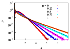
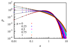
Figure 1: Semilogarithmic (top) and logarithmic (bottom) plot of the equilibrium distribution $p(x)$ of wealth $x$ for different values of $\mu$, i.e., for different fractions of unidirectional interactions. The value $\mu=0$ corresponds to immediate exchanges only and $\mu=1$ to the situation when all the interactions are unidirectional. Dots represent results from numerical simulations, while lines are a fitting using the $\varGamma$-distribution (8) with $\alpha$ given by Eq. (17) for different values of $\mu$.

While the model of Dr$\breve{\mathrm{a}}$gulescu and Yakovenko assumes that the total amount of wealth, $x_{j}+x_{k}$, is reshuffled randomly between the two interacting units, the first model introduced by Angle Angle1983a ; Angle1986a assumes a unidirectional flow: with probability $p_{0}$ a random fraction $\epsilon$ of the wealth $x_{j}$ of unit $j$ is transferred to unit $k$, while with probability $1-p_{0}$ a random fraction $\epsilon$ of the wealth $x_{k}$ of unit $k$ is transferred to unit $j$. Considering the particular case of the symmetrical interaction, i.e., $p_{0}=1/2$, then the dynamical evolution of the model is determined by Eqs. (1) with

$$\Delta x_{jk}=\epsilon[\eta x_{j}-(1-\eta)x_{k}]\,.$$ (14)

Here the stochastic variable $\eta$ can assume the values $0$ or $1$ with probability $1/2$; $\epsilon$ maintains the same meaning as above. In the case of the unidirectional wealth flow model of Angle, the growth of the fraction of poor units with wealth close to zero is even more dramatic than in the reshuffling dynamics considered above: in fact, the resulting equilibrium wealth distribution of this model is found to be a $\varGamma$-distribution with shape parameter $\alpha=1/2$ Katriel2014a , that diverges for $x\to 0$, signaling a wealth accumulation in the hands of a very few units.

When a saving propensity is introduced in this model, assuming that no wealth fraction greater than $(1-\lambda)$ can be transferred from one unit to the other, then Eq. (14) for the exchanged wealth becomes

$$\Delta x_{jk}=\epsilon(1-\lambda)[\eta x_{j}-(1-\eta)x_{k}]\,.$$ (15)

In this case, the equilibrium wealth distribution for a generic value of $\lambda$ is still described by a $\varGamma$-distribution with shape parameter Patriarca2010b

$$\alpha=\frac{1+2\lambda}{2(1-\lambda)}\,,$$ (16)

which is just half of the value given by Eq. (13) for the Chakraborti and Chakrabarti model. In this case, the divergence at $x\to 0$ will persist as long as $\alpha<1$, meaning saving propensities $\lambda<1/4$. At $\lambda=1/4$ the exponential distribution is obtained, while for $\lambda>1/4$ the distribution recovers the bell shape with mode $\bar{x}>0$. The value $\alpha=2$ of the immediate exchange model introduced above is recovered for $\lambda=1/2$.

One could expect that (at least in the case of symmetrical interactions) a long series of unidirectional wealth flows provides results equivalent to those produced by an analogous series of immediate (bidirectional) exchanges. However, the basic difference in the region at $x\to 0$ between the shapes of the equilibrium wealth distributions of the model of Angle and of the immediate-exchange model proposed here reveal that this is not the case. A better understanding of the latter issue can be obtained by investigating a system where at each time iteration the pair of units extracted for a trade will carry out with probability $\mu$ the unidirectional transaction defined by Eq. (14) and with probability $1-\mu$ the immediate exchange defined by Eq. (6).

If $\mu=0$, i.e., all interactions are immediate exchanges, the equilibrium wealth distribution is a $\varGamma$-distribution with $\alpha=2$. For any $\mu>0$ the equilibrium distributions are still well described for sufficiently large $x$ by a $\varGamma$-distribution, see Fig. 1. The dependence of $\alpha$ on $\mu$ is found to be given by

$$\alpha(\mu)=2\exp[-\ln(4)\mu]~{}=2^{1-2\mu}\,.$$ (17)

For $\mu=1/2$, i.e., when half of the interactions are unidirectional and half are immediate exchanges, $\alpha=1$ and the equilibrium wealth distribution is exponential, $f(x)=\exp(-x)$. For $x<0.05$ the distributions deviate from the $\varGamma$-distributions, see Fig. 1 for $x\to 0$; the deviation is the larger the larger is the fraction of unidirectional interactions, $\mu$. For $\mu=1$ the model described by Eqs. (1) and (14) is recovered.

Here, units making immediate exchanges a fraction $(1-\mu)$ of times can be interpreted as units with an effective saving propensity $\tilde{\lambda}(\mu)<\lambda$, where $\lambda$ is the value of the saving propensity of the Angle model, corresponding to $\mu=1$. The explicit relation between the effective saving propensity $\tilde{\lambda}(\mu)$ and the parameter $\mu$ can be found combining Eqs. (16) and (17),

$$\tilde{\lambda}(\mu)=\frac{2^{2(1-\mu)}-1}{2^{2(1-\mu)}+2}\,.$$ (18)

From here one can see that to $\mu=1$ corresponds $\lambda=0$, i.e., the units can lose everything during an exchange. Instead, $\mu=1/2$ leads to the same equilibrium distribution as the model of Angle with saving propensity $\lambda=1/4$, and $\mu=0$ to the equilibrium distribution with saving propensity $\lambda=1/2$. Distributions corresponding to values of $\lambda>1/2$ cannot be obtained, since they would correspond to negative values of $\mu$.

III The influence of a trading criterion

III.1 Formulation of the acceptance criterion

Let us now introduce a trading criterion on the basis of what each unit will decide whether to make the trade or not (in other kinetic wealth exchange models the two randomly chosen units always make the trade). The introduction of probabilistic factors influencing trades is a possible way to go beyond the assumption of perfect knowledge of the units assumed in neo-classical economic models. A probability law suitably describes the natural lack of perfect knowledge of the trading units concerning the product and its actual value measured as wealth, as well as the effect of personal feelings about the goods to be exchanged that can vary from time to time, or other external random perturbations affecting their decisions.

Here, the probabilistic acceptance criterion is assumed to depend only on the information currently available to the two trading units at the moment of the trade, i.e., we will use forms of acceptance criterion that depend on the wealths owned by the two interacting units before the (possible) trade and on the amount of wealth exchanged. Without loss of generality, one can focus on the generic unit $j$ that will be assumed to accept to carry out the trade with an acceptance probability $q_{j}$. As a simple example of acceptance probability we consider in the following the linear piece-wise function given by

$$q_{j}(\Delta x_{jk})=\begin{cases}0\,,&\mathrm{if}~{}\Delta x_{jk}<-\eta\langle x\rangle\,,\\ 1+\Delta x_{jk}/(\eta\langle x\rangle)\,,&\mathrm{if}~{}-\eta\langle x\rangle<\Delta x_{jk}<0\,,\\ 1\,,&\mathrm{if}~{}\Delta x_{jk}\geq 0\,.\end{cases}$$ (19)

Here $\eta$ is a parameter, $\langle x\rangle=\sum_{i=0}^{N}x_{i}/N$ is the average wealth of the system, and $\Delta x_{jk}$ is given by Eq. (6). This function is depicted as a continuous line in Fig. 2.

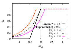
Figure 2: Examples of probability $q_{j}(\Delta x_{jk})$ that unit $j$ accepts to make a wealth exchange with unit $k$ leading to a net wealth variation $\Delta x_{jk}$ of unit $j$. Here “linear” refers to the piecewise linear probability in Eq. (19) for $\eta=1/2$, while the other “exponential” lines represent the probability given by Eq. (20) for $\eta=1/2$ and $\delta x_{0}=-0.2;0;0.2$. See text for details.

In this example, the criterion for accepting or not the exchange depends on the quantity $\eta\langle x\rangle$ and on the exchanged wealth $\Delta x_{jk}$. If $\Delta x_{jk}$ is negative (the unit $j$ is going to lose something) with $|\Delta x_{jk}|$ comparable with the scale $\eta\langle x\rangle$, then it is highly probable that there will be no trade as the unit $j$ who would lose is most likely not interested of the exchange. The exchange will certainly not take place if $|\Delta x_{jk}|>\eta\langle x\rangle$. If $\Delta x_{jk}$ is still negative but with $|\Delta x_{jk}|$ not too large compared to the scale $\eta\langle x\rangle$ then it is possible that unit $j$ will accept the exchange anyway, even though losing something. The latter situation could correspond, e.g., to a situation in which he is not capable to estimate the loss, or he is simply interested in the other object for whatever reason and therefore is ready to accept a limited loss. For $\Delta x_{jk}>0$ unit $j$ will always accept the exchange. Both trading units $j$ and $k$ will independently adopt the same criterion, the criterion of unit $k$ being defined by an analogous function $q_{k}(\Delta x_{kj})=q_{j}(-\Delta x_{jk})$ obtained from the function given by Eq. (19) by exchanging $k$ and $j$ and, correspondingly, $\Delta x_{kj}$ with $-\Delta x_{jk}$. The decision of each agent $k$ or $j$ is taken probabilistically with the help of an additional random number that is extracted independently and compared with $q_{j}(\Delta x_{jk})$ or $q_{k}(\Delta x_{kj})$ for the decisions of unit $j$ and $k$, respectively. Since the quantity $\Delta x_{jk}=\epsilon_{k}x_{k}-\epsilon_{j}x_{j}$ is given as the difference between the values $\epsilon_{k}x_{k}$ and $\epsilon_{j}x_{j}$ of the wealth goods exchanged, it represents an actual measure of the profit or loss of a unit in an exchange. Thus, the type of interaction between units formulated above is expected to simulate an actual barter or trade realistically, since whether the units will carry out the exchange or not depends on their corresponding profit or loss.

It is possible to construct similar functions with specific properties and depending on additional parameters. We employ in the following some other forms of the acceptance probability function, in particular the following exponential shape,

$$q_{j}(\Delta x_{jk})=\begin{cases}\exp[(\Delta x-\delta x_{0})/(\eta\langle x\rangle)]\,,&~{}\mathrm{if}~{}\Delta x_{jk}<\delta x_{0}\,,\\ 1\,,&~{}\mathrm{if}~{}\Delta x_{jk}\geq\delta x_{0}\,.\end{cases}$$ (20)

This probability function has an exponential shape for $\Delta x_{jk}<\delta x_{0}$ and is equal to $1$ otherwise. The shapes of the curve corresponding to an acceptance parameter $\eta=0.5$ and shift parameters $\delta x_{0}=0,\pm 0.2$ are shown in Fig. 2. The parameter $\delta x_{0}$ can be used to make the acceptance criterion stricter or looser — notice that an analogous parameter can in principle be introduced in any other function $q_{j}(\Delta x_{jk})$. The acceptance criterion become looser for $\delta x_{0}<0$, when a unit can accept to carry out an exchange even if accompanied by a limited loss of the order of $|\delta x_{0}|$. Instead, the criterion becomes stricter for $\delta x_{0}>0$, since in this case trades are accepted with certainty only if the gain is larger than the threshold value $\delta x_{0}$.

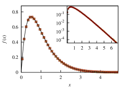
Figure 3: Equilibrium wealth distributions $f(x)$ of the immediate-exchange model. All the distributions obtained using different or no acceptance criteria (dots) collapse on the same $\varGamma$-distribution $f_{\alpha}(x)$ with $\alpha=2$ (continuous curve). The criteria used employ (a) the “linear” probability in Eq. (19) with $\eta=0.1;0.5;1;5;10;$ and (b) the “exponential” probability in Eq. (20) with $\eta=0.5$ and $\delta x_{0}=-0.4;-0.2;0;0.2;0.4$. Inset: same plot in semilogarithmic scale.

III.2 Acceptance criterion in the immediate exchange model

We start by applying the acceptance criterion (19) to the kinetic model of immediate exchange introduced in Sect. II. The equilibrium distributions of wealth obtained after adding the acceptance criterion turns out to be a $\varGamma$-distribution (8), namely the distribution $f_{2}(x)$ with the same shape parameter $\alpha=2$ independently of the value of $\eta$. Thus, the shape of the equilibrium wealth distribution remains unchanged with respect to the case in which no acceptance criterion is used.

This is true also when different acceptance criteria are employed. The equilibrium wealth distributions obtained employing the piece-wise linear function (19) and those corresponding to the exponential acceptance probability function (20) for different values of the shift parameter $\delta x_{0}$ are compared with each other and with the analytical shape of the distribution $f_{2}(x)$ in Fig. 3.

The value of $\eta$ in Eqs. (19) and (20) as well that of $\delta x_{0}$ in Eq. (20) change the relaxation process to equilibrium Patriarca2007a (e.g. a smaller $\eta$ corresponds to a larger relaxation time) but surprisingly do not have any importance for the equilibrium wealth distribution, that is exactly the same one obtained when assuming that the two randomly chosen units make the trade with probability $q\equiv 1$.

III.3 Asymmetrical acceptance criteria

The considerations above lead to the conclusion that introducing a decision making process that can be interpreted as the trial to introduce intelligence in the units behavior, is irrelevant for the final state of the system. However, this is true only as long as the acceptance criterion is formulated symmetrically with respect to the two trading units. Different asymmetrical criteria lead to different forms of the equilibrium wealth distribution and to shapes of the equilibrium wealth distributions different from $\varGamma$-distributions. Such asymmetrical criteria can be of interest in the study of preferential attachment effects, e.g., when considering the influence of the richness of the two trading units on the outcome of the trade. That is the case of the so-called “rich get richer effect” already considered in the model of Angle Angle1986a , characterized by uni-directional wealth flows taking place with a higher probability from the poorer to the richer unit. Notice that unidirectional models represent actual realizations of the so-called “Matthew effect” Merton1968a , since during an encounter not only the richer unit becomes richer with a higher probability but correspondingly, due to wealth conservation, the poorer unit becomes even poorer.

As a test, we have studied an asymmetrical version of the immediate exchange model discussed above, in which a criterion favoring richer units was introduced by always allowing trades with a gain for the richer trading unit and preventing trades accompanied by a net gain of the poorer unit a fraction $\theta$ of times, $0\leq\theta\leq 1$.

In Fig. 4 the equilibrium wealth distribution for some values of $\theta$ ranging between $\theta=0$ (corresponding to symmetrical exchanges) and $\theta=0.9$ (representing a strong asymmetry in the exchange criterion) are shown. One can observe how the number of units in the small-$x$ region increases with $\theta$ and that, correspondingly, the distribution mode shifts leftwards. It is to be noticed that for high enough values of $\theta$ the distribution diverges for $x\to 0$ — Fig. 4 shows such a case for $\theta=0.9$. Most importantly, the shapes of the equilibrium distributions obtained for $\theta>0$ are not well fitted anymore by a $\varGamma$-distribution (comparison not shown).

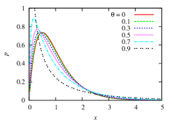
Figure 4: Equilibrium wealth distribution obtained using an asymmetrical criterion for different fractions $\theta$ of trades that would be advantageous for the richer unit; see text for details. Equilibrium distributions with $\theta>0$ are not well fitted by a $\varGamma$-distribution (comparison not shown).

III.4 Acceptance criteria in other models: relative acceptance criteria

In order to check for other instances of the invariance properties found above for the immediate-exchange model, we have numerically investigated the effects of an acceptance criterion in other kinetic exchange models, namely in the Dr$\breve{\mathrm{a}}$gulescu-Yakovenko Dragulescu2000a and in the Chakraborti-Chakrabarti model with saving propensity Chakraborti2000a .

We start from the Dr$\breve{\mathrm{a}}$gulescu-Yakovenko model, defined by Eqs. (10) or by Eqs. (1) with (9), whose equilibrium wealth distribution is a simple exponential shape, $f(x)=\exp(-x)$ (if $\langle x\rangle=1$) Dragulescu2000a . In fact, we find that the exponential form remains unchanged, independently of the form of the symmetrical acceptance criterion used, such as those defined by Eqs. (19) or (20). The independence from the acceptance criteria widens the validity range and justifies the use of the original minimal version of the model where no acceptance criterion is present, instead of more elaborate versions where units follow more “intelligent” principles.

However, the independence of the equilibrium distribution of a symmetrical acceptance criterion does not hold for the Chakraborti-Chakrabarti model with saving propensity Chakraborti2000a . In this case one obtains a different equilibrium wealth distribution, that cannot be fitted anymore by a $\varGamma$-distribution.

Considering the homogeneity of the update rules of the model, we have checked the effect of a probabilistic constraint on the relative variable $\Delta x_{jk}/x_{j}$ of unit $j$ rather than on the absolute wealth exchange $\Delta x_{jk}$, finding that a good fitting of the equilibrium wealth distributions through a $\varGamma$-distribution is recovered in this case. In other words, if in the Chakraborti-Chakrabarti model with a given saving propensity $\lambda$ an acceptance criterion is introduced, defined in terms of an (arbitrary) acceptance probability function $Q_{j}$ for each unit $j$ depending on the relative amount of wealth exchanged $\Delta x_{jk}/x_{j}$, then the equilibrium wealth distribution is still a $\varGamma$-function, but with a shape parameter different from the value given by Eq. (13). For clarity we discuss only the acceptance criterion defined by the acceptance probability $Q_{j}$ obtained by modifying the piece-wise linear acceptance probability $q_{j}$ in Eq. (19),

$$Q_{j}(\Delta x_{jk}/x_{j})\!=\!\begin{cases}0\,,&\mathrm{if}~{}\Delta x_{jk}/x_{j}<-\eta,\\ 1\!+\!\Delta x_{jk}/(\eta\,x_{j}),&\mathrm{if}~{}-\eta\!<\!\Delta x_{jk}/x_{j}\!<\!0,\\ 1\,,&\mathrm{if}~{}\Delta x_{jk}\geq 0\,.\end{cases}$$ (21)

The rescaled variable $\Delta x_{jk}/x_{j}$ has the new range $(-1,1)$. Results are summarized in Fig. 5-top, showing the new shape parameter $\alpha_{q}$ of the $\varGamma$-distribution $f_{\alpha_{q}}(x)$ fitting the equilibrium wealth distribution versus the corresponding value of the saving propensity $\lambda$ of the model, for different values of the acceptance parameter $\eta$. In the limit of very large values of $\eta$, in which the acceptance criterion become very loose and becomes equivalent to no criterion present, results reduce to those of the original Chakraborti-Chakrabarti model, represented by the continuous line representing $\alpha(\lambda)$ of Eq. (13); in all other cases one has $\alpha_{q}>\alpha(\lambda)$.

The results can also be expressed by saying that the relative acceptance criterion with acceptance parameter $\eta$, defined by Eqs. (21), turns the equilibrium wealth distribution of the Chakraborti-Chakrabarti model with saving propensity $\lambda$ into that of the same model with a different saving propensity $\lambda_{q}$. The value of the effective saving propensity $\lambda_{q}$ corresponding to the observed $\alpha_{q}$ can be obtained inverting the relation (13) and is given by

$$\lambda_{q}=(\alpha_{q}-1)/(\alpha_{q}+2)\,.$$ (22)

For convenience the values of $\lambda_{q}$ are depicted in Fig. 5-bottom. It is clear that for every value of the acceptance parameter $\eta$ one has $\lambda_{q}>\lambda$, i.e., the use of an acceptance criterion is equivalent to a larger saving propensity. For large values of $\eta$, when the acceptance criterion becomes very loose, results reduce to the original Chakraborti-Chakrabarti model without acceptance criterion and $\lambda_{q}\to\lambda$.

A surprising point implied by these results is that the saving propensity of the Chakraborti-Chakrabarti model can be generated by introducing a relative acceptance criterion. In fact, the considerations above also apply to the Dr$\breve{\mathrm{a}}$gulescu-Yakovenko model, that is obtained from the Chakraborti-Chakrabarti model in the limit $\lambda\to 0$. Thus, one can start from the Dr$\breve{\mathrm{a}}$gulescu-Yakovenko model without saving propensity and obtain the same equilibrium distribution of the Chakraborti-Chakrabarti model with arbitrary saving propensity $\lambda$, corresponding to the dots at $\lambda=0$ in Fig. 5, through the use of an acceptance criterion with a suitable value of $\eta$. This justifies at the microscopic level of the decision processes, carried out by the units before an exchange, the use of a saving propensity $\lambda>0$ inserted “by hand” in the Chakraborti-Chakrabarti model as a convenient numerical or effective statistical procedure.

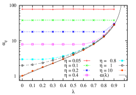
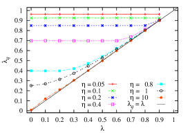
Figure 5: Fitting of the equilibrium wealth distribution of the Chakraborti-Chakrabarti model with acceptance criterion defined by Eq. (21) through a $\varGamma$-distribution. Top: shape parameter $\alpha_{q}$ versus saving parameter $\lambda$ for different acceptance parameters $\eta$. The black solid line is the value of $\alpha(\lambda)$ given by Eq. (13), corresponding to the Chakraborti-Chakrabarti model, recovered in the $\eta\to\infty$ limit, i.e., when there is no acceptance criterion. Bottom: effective saving parameter $\lambda_{q}$ corresponding to the values of $\alpha_{q}$ in the top panel. In general $\lambda_{q}>\lambda$. In the limit of large $\eta$ the presence of an acceptance criterion becomes negligible and $\lambda_{q}\to\lambda$.

IV Heterogeneous immediate-exchange model

In this section we investigate the generalization of the homogeneous model studied above to the heterogeneous case, when each unit behaves according to a different trading criterion. As in the homogeneous case, the presence of a heterogeneity in the parameter values can be related to specific features of the units, such as the efficiency of the trading strategy employed by the units or their education level Angle2006a .

Here, we limit ourselves to consider an absolute acceptance criterion. In fact, while the equilibrium distribution of a homogeneous system is invariant under change of the form of the (symmetrical) criterion employed, the presence of a heterogeneity level in the system parameters is sufficient to break this invariance. The same piece-wise linear probability function considered above is used, but now each unit $j$ ($j=1,\dots,N)$ is characterized by a different parameter $\eta_{j}$. The corresponding acceptance probability function is given by

$$q_{j}(\Delta x_{jk})\!=\!\begin{cases}0\,,&\!\!\!\mathrm{if}~{}\Delta x_{jk}<-\eta_{j}\langle x\rangle,\\ 1+\Delta x_{jk}/(\eta_{j}\langle x\rangle)\,,&\!\!\!\mathrm{if}~{}-\eta_{j}\langle x\rangle<\Delta x_{jk}<0,\\ 1\,,&\!\!\!\mathrm{if}~{}\Delta x_{jk}\geq 0.\end{cases}$$ (23)

The equilibrium distribution does not have a universal shape anymore and depends on the specific acceptance parameters $\{\eta_{i}\}$ used or on their distribution $\phi(\eta)$ that can be defined in the limit of a large number of units.

It to be noticed that heterogeneity does not concern the functional form of the amount of exchanged wealth $\Delta x_{jk}$ but enters the model through the parameters of the acceptance criterion used by each unit.

We have investigated various forms of distributions $\phi(\eta)$. The equilibrium wealth distributions obtained from uniform threshold distributions with parameters $\eta_{i}$ randomly extracted in an interval $(\eta_{\mathrm{min}},\eta_{\mathrm{max}})$ in general are not realistic. An example of such equilibrium wealth distributions obtained for a fixed $\eta_{\mathrm{min}}=0.1$ and different values of $\eta_{\mathrm{max}}$ are plotted in Fig. 6. One can notice that when thresholds are very limited in the range (all close to $\eta=0.1$ in the example of Fig. 6) the model is almost homogeneous and one recovers a $\varGamma$-distribution. The presence of a significant fraction of agents $i$ with higher values of the parameter $\eta_{i}$ produces a depletion of the distribution in the intermediate wealth zone and an enhancement of the concentration of units both at small and large values of wealth. In the large-wealth region one can notice the formation of a new maximum that can be interpreted as the formation of a rich class made of the units with the smallest values of $\eta_{i}$’s. To the best of our knowledge this type of maximum is not observed in real data of wealth distributions.

Results reproducing a realistic shape of wealth distributions, are obtained by following a simple recipe consisting in constructing a system in which the majority of units has a standard or low performance during trading interactions and a small fraction of units perform much better. This prescription was already tested in Ref. Patriarca2006c in the framework of the Chakraborti-Chakrabarti model with saving propensities Chakraborti2000a by assigning a zero saving propensity to 99% of the population and higher saving propensities, uniformly distributed in $\lambda\in(0,1)$, to the remaining 1% of the population. This led to realistic shapes of wealth distribution, see Ref. Patriarca2006c for details. The recipe is here adapted to the immediate-exchange model under consideration by assigning a (fixed) larger parameter value $\eta_{i}\equiv\bar{\eta}=2$ to a majority (95%) of the population — here a larger value of $\eta$ corresponds to a looser criterion used in accepting an exchange, while the remaining 5% of the population is assigned a set of smaller parameters $\eta_{i}$ uniformly extracted in the interval $\eta\in(0.5,0.7)$. The resulting equilibrium wealth distribution, shown in Fig. 7, indeed presents the stylized features of wealth distributions, such as a mode $x_{\mathrm{m}}>0$ and a Pareto power-law at larger values of wealth with a Pareto index $p\approx 2$.

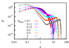
Figure 6: Equilibrium distribution $f(x)$ of wealth $x$ of a system of heterogeneous units with diversified acceptance parameters $\{\eta_{i}\}$ uniformly distributed in the interval $(\eta_{\mathrm{min}},\eta_{\mathrm{max}})$, for $\eta_{\mathrm{min}}=0.1$ and different values of $\eta_{\mathrm{max}}$.

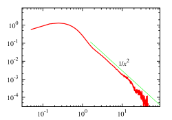
Figure 7: Equilibrium distribution $f(x)$ of wealth $x$ of a system of heterogeneous units with diversified acceptance parameters $\{\eta_{i}\}$: 95% of the units has $\eta=2$, while the remaining 5% has $\{\eta_{i}\}$ uniformly distributed in $\eta\in(0.5,0.7)$.

V Conclusions

In the present paper we have proposed a model of wealth exchange aimed at overcoming some critics raised about the kinetic exchange models, laying down firmer foundations for the models themselves, and providing a more realistic description of a trade between two economic units. Doing this, two main features of the original models have been modified. First, an immediate-exchange wealth dynamics has been introduced, describing two actual and distinct wealth flows taking place during the same interaction between two economic units, just as in an actual trade. Models, where the total wealth is randomly reshuffled between the two units or which follow a uni-directional dynamics, better represent exchanges of valuables without the demand of an immediate reward, as, e.g., in gift economies. Immediate bidirectional exchanges produce more realistic shapes of wealth distribution $f(x)$, such that $f(0)=0$ and having a mode larger than zero. Furthermore, the model is made more realistic at a microeconomic level, allowing units to decide whether to trade or not, according to some criterion based on the profit gained from the trade. Criteria formulated symmetrically with respect to the two trading units — but arbitrary for the rest — preserve some symmetries of the model. In the immediate-exchange models as well as in the Dr$\breve{\mathrm{a}}$gulescu-Yakovenko model, a symmetrical criterion does not change the equilibrium wealth distribution at all.

In the case of the Chakraborti-Chakrabarti model, when a symmetrical acceptance condition on the relative wealth is used, one still finds that the equilibrium distribution is a $\varGamma$-distribution, but with a larger value of the shape parameter $\alpha$, corresponding to a higher saving propensity $\lambda$. This implies interesting links between different kinetic exchange models and provides at the same time a microscopic justification. For example, the equilibrium distribution of the Chakraborti-Chakrabarti model can also be obtained from the reshuffling dynamics of the Dr$\breve{\mathrm{a}}$gulescu-Yakovenko model with the addition of an acceptance criterion with suitable parameters.

The situation changes either when the criterion depends asymmetrically on the wealths of the two units (also in homogeneous systems) or in the case of heterogeneous systems, where there is anyway a situation of asymmetry due to the fact that each unit uses a different criterion. In these cases the equilibrium wealth distribution depends on the specific set of criteria used by units. The heterogeneous version of the bidirectional model presents a wide spectrum of possible shapes for the equilibrium wealth distribution. We have found that realistic shapes, presenting a Pareto power-law, are obtained for moderate levels of heterogeneity.

In order to provide quantitative explanations of the many regularities of and links between the various models discussed above it would be important that future work advances also toward the analytical solution of kinetic exchange models. Furthermore, while the ubiquitous presence of the $\varGamma$-distribution can be related to the validity of the Boltzmann theorem, due to the conservation of wealth during trades, it would be relevant to gain some information also on the analytical shapes of the equilibrium wealth distributions when the Boltzmann theorem does not apply, e.g. in the interesting Maxwell-demon-type dynamics Apenko2014a corresponding to cases of asymmetrical acceptance criteria describing e.g. the “rich gets richer” effect.

References

- (1) M. Patriarca, E. Heinsalu, A. Chakraborti, Eur. Phys. J. B 73, 145 (2010)
- (2) M. Patriarca, A. Chakraborti, Am. J. Phys. 81(8), 618 (2013), http://link.aip.org/link/?AJP/81/618/1
- (3) J. Angle, Social Forces 65, 293 (1986)
- (4) J. Angle, J. Math. Sociol. 17, 77 (1992)
- (5) J. Angle, Physica A 367, 388 (2006)
- (6) E. Bennati, La simulazione statistica nell’analisi della distribuzione del reddito: modelli realistici e metodo di Monte Carlo (ETS Editrice, Pisa, 1988)
- (7) E. Bennati, Rivista Internazionale di Scienze Economiche e Commerciali 35, 735 (1988)
- (8) E. Bennati, Rassegna di lavori dell’ISCO X, 31 (1993)
- (9) A. Dragulescu, V.M. Yakovenko, Eur. Phys. J. B 17, 723 (2000)
- (10) A. Dragulescu, V.M. Yakovenko, Physica A 299, 213 (2001)
- (11) A. Dragulescu, V.M. Yakovenko, Eur. Phys. J. B 20, 585 (2001)
- (12) V. Yakovenko, J. J. Barkley Rosser, Rev. Mod. Phys. 81, 1703 (2009)
- (13) A. Chakraborti, B.K. Chakrabarti, Eur. Phys. J. B 17, 167 (2000)
- (14) A. Chakraborti, Int. J. Mod. Phys. C 13(10), 1315 (2002)
- (15) E. Samanidou, E. Zschischang, D. Stauffer, T. Lux, Rep. Prog. Phys. 70, 409 ((2007)
- (16) A. Chatterjee, S. Yarlagadda, B.K. Chakrabarti, eds., Econophysics of Wealth Distributions - Econophys-Kolkata I (Springer, 2005)
- (17) B. Hayes, Am. Sci. 90(5), 400 (2002)
- (18) T. Lux, Emergent Statistical Wealth Distributions in Simple Monetary Exchange Models: A Critical Review, in Econophysics of Wealth Distributions, edited by A. Chatterjee, S.Yarlagadda, B.K. Chakrabarti (Springer, 2005), p. 51
- (19) A.S. Chakrabarti, B.K. Chakrabarti, Physica A 388, 4151 (2009)
- (20) L. Lü, M. Medo, Y.C. Zhang, D. Challet, Eur. Phys. J. B 64, 293 (2008)
- (21) H. Liao, R. Xiao, D. Chen, M. Medo, Y.C. Zhang, Physica A 400, 47 (2014)
- (22) M.A. Miceli, F. Cecconi, Cerulli, Working Papers 161, University of Rome La Sapienza, Department of Public Economics (2013), http://ideas.repec.org/p/sap/wpaper/wp161.html
- (23) M. Mauss, The Gift (Routlege, London, 1950)
- (24) A. Salem, T. Mount, Econometrica 42, 1115 (1974)
- (25) A. Chakraborti, M. Patriarca, Pramana J. Phys. 71, 233 (2008)
- (26) M. Patriarca, A. Chakraborti, K. Kaski, Physica A 340, 334 (2004)
- (27) M. Patriarca, A. Chakraborti, K. Kaski, Phys. Rev. E 70, 016104 (2004)
- (28) M. Patriarca, A. Chakraborti, K. Kaski, G. Germano, Kinetic theory models for the distribution of wealth: Power law from overlap of exponentials, in Econophysics of Wealth Distributions, edited by A. Chatterjee, S.Yarlagadda, B.K. Chakrabarti (Springer, 2005), p. 93
- (29) S. Apenko, arXiv:1404.6729 [cond-mat.stat-mech] (2014)
- (30) J. Angle, The surplus theory of social stratification and the size distribution of personal wealth, in Proceedings of the American Social Statistical Association, Social Statistics Section (Alexandria, VA, 1983), pp. 395–400
- (31) G. Katriel, arXiv:1404.4068 [q-fin.GN] (2014)
- (32) M. Patriarca, A. Chakraborti, E. Heinsalu, G. Germano, Eur. J. Phys. B 57, 219 (2007)
- (33) R.K. Merton, Science 159(3810), 56 (1968)
- (34) M. Patriarca, A. Chakraborti, G. Germano, Physica A 369, 723 (2006)