Multiscale nature of the dissipation range in gyrokinetic simulations of Alfvénic turbulence

Abstract

Nonlinear energy transfer and dissipation in Alfvén wave turbulence are analyzed in the first gyrokinetic simulation spanning all scales from the tail of the MHD range to the electron gyroradius scale. For typical solar wind parameters at 1 AU, about 30% of the nonlinear energy transfer close to the electron gyroradius scale is mediated by modes in the tail of the MHD cascade. Collisional dissipation occurs across the entire kinetic range $k_{\perp}\rho_{i}\gtrsim 1$. Both mechanisms thus act on multiple coupled scales, which have to be retained for a comprehensive picture of the dissipation range in Alfvénic turbulence.

Introduction. Spacecraft measurements find a radial temperature profile of the solar wind which can only be explained by the presence of heating throughout the heliosphere (Richardson and Smith, 2003). The key mechanism of heating in the inner heliosphere up to $\sim$20 AU is thought to be the dissipation of turbulent fluctuation energy, and its understanding and description is one of the outstanding open issues in space physics (Bruno and Carbone, 2013). Over the past decade, numerous studies, both observational (Bale et al., 2005; Alexandrova et al., 2009; Sahraoui et al., 2009, 2010; Chen et al., 2013) and theoretical/computational (Howes et al., 2008, 2011a; Wan et al., 2012; Salem et al., 2012; TenBarge et al., 2013; TenBarge and Howes, 2013; Osman et al., 2014), have focused on this topic, extracting ever more sophisticated measurements of solar wind fluctuation properties, and accomplishing increasingly detailed turbulence simulations.

As the solar wind plasma is only weakly collisional, a variety of kinetic effects such as cyclotron damping, Landau and transit time damping, finite Larmor radius effects, stochastic heating, or particle acceleration at reconnection sites can contribute to the conversion of field energy to particle energy, and thus determine how collisional dissipation will ultimately set in. A kinetic description is crucial in order to judge the relative importance of each of those effects. Due to the complexity of a nonlinear kinetic system, numerical simulations are essential to interpret observations and provide guidance for analytical theory.

In the present Letter, we employ an approach based on gyrokinetic (GK) theory (Brizard and Hahm, 2007), which is a rigorous limit of kinetic theory in strongly magnetized plasmas. Due to the assumptions of low frequencies (compared to the ion cyclotron frequency) and small fluctuation levels, the gyrokinetic model excludes cyclotron resonances and stochastic heating. In absence of these effects, we focus on the energetic properties of kinetic Alfvén wave (KAW) turbulence, which has been demonstrated to be a crucial ingredient of solar wind turbulence (Podesta, 2013).

We address the following key questions: (1) Which spectral features can be found in a comprehensive simulation extending from the magnetohydrodynamic (MHD) range down to the electron gyroradius scale? (2) What are the characteristics of nonlinear energy transfer from large to small scales? (3) How is energy dissipated, and how is the dissipated energy partitioned between ions and electrons?

Simulation setup. The nonlinear GK system of equations is solved using the Eulerian code $\mathrm{GENE}$ (Jenko et al., 2000) to study the dynamics of KAW turbulence in three spatial dimensions. In order to model the energy injection at the outer scales of the system, a magnetic antenna potential, whose amplitude is evolved in time according to a Langevin equation (TenBarge et al., 2014), is externally prescribed at the largest scales of the simulation domain. The driven modes are $\left(0,1,\pm 1\right)$ and $\left(1,0,\pm 1\right)$, where $\left(i,j,k\right)$ are multiples of the lowest wave numbers in $\left(k_{x},k_{y},k_{z}\right)$, respectively. The mean antenna frequency is chosen to be $\omega_{a}=0.9\omega_{A0}$ ($\omega_{A0}$ being the frequency of the slowest Alfvén wave in the system), the decorrelation rate is set to $\gamma_{a}=0.7\omega_{A0}$, and the normalized antenna amplitude is set to $A_{\|,0}=\omega_{A0}B_{0}\sqrt{\delta}/C_{2}k_{\perp 0}^{2}\sqrt{N}v_{A}$ (setting $\delta=2,$ $N=4$, $C_{2}=1$), in accordance with the critical balance condition $\omega_{\mathrm{lin}}\sim\omega_{\mathrm{nl}}$ (TenBarge et al., 2014).

The physical parameters are chosen to be similar to solar wind conditions at 1 AU, with $\beta_{i}=8\pi n_{i}T_{i}/B_{0}^{2}=1$, $T_{i}/T_{e}=1$. Proton and electron species are included with their real mass ratio of $m_{i}/m_{e}=1836$. The electron collisionality is chosen to be $\nu_{e}=0.06\omega_{A0}$ (with $\nu_{i}=\sqrt{m_{e}/m_{i}}\nu_{e}$), a value small enough to not inhibit kinetic effects, but large enough to reduce resolution requirements in velocity space.

In order to maximize the effective dynamic range, the simulation domain is extended significantly compared to previously published work, to include scales larger than the ion gyroradius, allowing for a free distribution of energy into the KAW or the ion entropy cascade (Schekochihin et al., 2009) as the ion gyroradius scale is passed. The evolution of the gyrocenter distribution is tracked on a grid with the resolution $\left(n_{x},n_{y},n_{z},n_{v_{\|}},n_{\mu},n_{\sigma}\right)=\left(512,512,96,48,15,2\right).$ The plane perpendicular to the background magnetic field is resolved by $512^{2}$ fully dealiased grid points, covering a perpendicular wavenumber range $0.2\leq k_{\perp}\rho_{i}\leq 51.2$ (or $0.0047\leq k_{\perp}\rho_{e}\leq 1.19$), thus extending into the regime where electron finite-Larmor-radius effects become important. Here, $\rho_{\sigma}=\sqrt{T_{\sigma}m_{\sigma}}c/eB$ with the species index $\sigma$. The number of grid points in the perpendicular plane is thus increased by a factor of 36 with respect to the largest runs of this kind published to date (Howes et al., 2011a). 96 points are used to resolve the dynamics along the background field (the $z$ direction), and $48\times 15$ gridpoints are chosen to represent the $\left(v_{\|},\mu\right)$ domain, where $v_{\|}$ is the velocity along the guide field, and $\mu=mv_{\perp}^{2}/2B_{0}$ is the magnetic moment with respect to the guide field. The domain sizes in velocity space are chosen to extend up to 3 thermal velocities $v_{T\sigma}$ in both parallel and perpendicular velocities for each species $\sigma$, where $v_{T\sigma}=\sqrt{2T_{\sigma}/m_{\sigma}}$.

Our simulations are performed using the same iterative expansion scheme as in Ref. (Howes et al., 2011a), where simulations are initially run with low resolution and are then restarted several times with an increasingly fine grid, until the target resolution is reached. The total runtime is chosen to span several antenna oscillation periods $\tau_{A}$ (in this case $t_{\mathrm{end}}=7.20\tau_{A}$) in order to ensure that a quasi-steady state has been reached.

Diagnostic methods. The key results of this study are obtained using a set of sophisticated energy diagnostics (partially introduced in Refs. (Bañón Navarro et al., 2011a, b; Teaca et al., 2012, 2014)), which enable studies of energy source, transfer and dissipation spectra separately for each species, and which are applied to KAW turbulence for the first time here. In particular, we analyze the time derivative of the spatially averaged free energy density, which can be expressed in the case of an antenna-driven electromagnetic system as

$$\partial_{t}\mathcal{E} = \Re\sum_{\sigma}\sum_{\boldsymbol{k}}\left\langle\frac{2\pi B_{0}}{m_{\sigma}}\int\mathrm{d}\mu\mathrm{d}v_{\|}\left(h_{\sigma\boldsymbol{k}}\frac{T_{0\sigma}}{F_{0\sigma}}\right.\right.$$ (1)

$$+ \left.\frac{q_{\sigma}v_{\|}}{c}\mathcal{C}\overline{A}_{\mathrm{\|ant},\sigma\boldsymbol{k}}\biggr{)}^{*}\partial_{t}g_{\sigma\boldsymbol{k}}\right\rangle$$

$$+ \Re\sum_{\boldsymbol{k}}\left\langle\frac{k_{\perp}^{2}}{4\pi}A_{1\|\mathrm{tot},\boldsymbol{k}}^{*}\partial_{t}A_{\|\mathrm{ant},\boldsymbol{k}}\right\rangle.$$

Here, the sum over $\boldsymbol{k}$ denotes a summation over all wavenumber pairs $\left(k_{x},k_{y}\right)$, and the angle brackets indicate a spatial average along the guide field. $f_{\sigma\boldsymbol{k}}$ is the perturbed gyrocenter distribution, and $h_{\sigma\boldsymbol{k}}=f_{\sigma\boldsymbol{k}}+\left(q_{\sigma}\overline{\phi}_{1\sigma\boldsymbol{k}}+\mu\overline{B}_{1\|\sigma\boldsymbol{k}}\right)F_{0\sigma}/T_{0\sigma}$ is its nonadiabatic part. The overbar denotes an average over the gyro-ring, and $F_{0\sigma}$ is a Maxwellian background distribution with background density $n_{0\sigma}$ and temperature $T_{0\sigma}$. The magnetic potential $A_{1\|\mathrm{tot},\boldsymbol{k}}=A_{1\|\boldsymbol{k}}+A_{\|\mathrm{ant},\boldsymbol{k}}$ is understood to contain also the contribution due to the Langevin antenna $A_{\|\mathrm{ant},\boldsymbol{k}}$, which is necessary for a complete account of the energy contained in the system. The time derivative $\partial_{t}g_{\sigma\boldsymbol{k}}=\partial_{t}(f_{\sigma\boldsymbol{k}}+q_{\sigma}v_{\|}\overline{A}_{1\|\boldsymbol{k}}F_{0\sigma}/cT_{0\sigma})$ is the quantity explicitly evolved in the GK Vlasov equation as implemented in GENE, and

$$\mathcal{C}=k_{\perp}^{2}\biggl{/}\left(k_{\perp}^{2}+\sum_{\sigma}\frac{8\pi^{2}q_{\sigma}^{2}B_{0}}{m_{\sigma}c^{2}T_{0\sigma}}\int v_{\|}^{2}J_{0}^{2}\left(\lambda_{\sigma}\right)F_{0\sigma}\mathrm{d}v_{\|}\mathrm{d}\mu\right)$$

is a factor arising from the antenna-modified Ampere’s law, with $\lambda_{\sigma}=k_{\perp}\sqrt{2m_{\sigma}\mu/B_{0}q_{\sigma}^{2}}$. By replacing $\partial_{t}g_{\sigma\boldsymbol{k}}$ in Eq. (1) with any of the various terms contributing to its evolution, we can assess the impact of that term on the evolution of the free energy density. The nonlinear transfer function (i.e. the free energy balance contribution of the nonlinear term) thus reads

$$T_{\boldsymbol{kpq}} = \frac{\pi B_{0}}{m_{\sigma}}\Re\int\mathrm{d}v_{\|}\mathrm{d}\mu\left[p_{x}q_{y}-p_{y}q_{x}\right]\left[\overline{\chi}_{1\sigma\boldsymbol{p}}h_{\sigma\boldsymbol{q}}-\overline{\chi}_{1\sigma\boldsymbol{q}}h_{\sigma\boldsymbol{p}}\right]$$ (2)

$$\times \left[h_{\sigma\boldsymbol{k}}\frac{T_{0\sigma}}{F_{0\sigma}}+q_{\sigma}v_{\|}\mathcal{C}\overline{A}_{\mathrm{\|ant},\sigma\boldsymbol{k}}/c\right],$$

with $\boldsymbol{k}+\boldsymbol{p}+\boldsymbol{q}=0$. Compared to the definition used in Refs. (Teaca et al., 2012, 2014), there is an additional term involving the antenna potential, and the electrostatic approximation has been dropped by using the full electromagnetic potential $\overline{\chi}_{1\sigma}=\overline{\phi}_{1\sigma}-v_{\|}\overline{A}_{1\|\mathrm{tot},\sigma}/c+\mu\overline{B}_{1\|\sigma}/q_{\sigma}$. Note that the new antenna potential term does not satisfy the same symmetry properties as the rest of the transfer function, consistent with the fact that the antenna acts as an energy source through the nonlinear term (but also through the parallel advection term). This source can be quantified by measuring the symmetric part of the above transfer function.

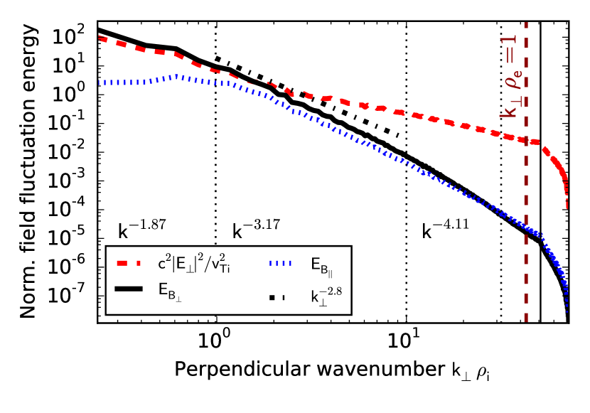
Figure 1: Normalized field energy spectra. Power law exponents obtained from the $B_{\perp}$ energy spectra within the dotted sections are printed into the plot.

Field energy spectra. Before focusing on the nonlinear transfer physics, we analyze the spectra of the magnetic and electric field energy, which can be directly compared to spacecraft observations. As is common practice, we compute 1-D spectra of $E_{E_{\perp}},$ $E_{B_{\|}}$, and $E_{B_{\perp}}$ vs. $k_{\perp}\rho_{i}$ by summing the energy of all $\left(k_{x},k_{y}\right)$ modes within a given $k_{\perp}$ shell. Shells are linearly spaced and divided into 384 bins; a short-time average over about $0.01\tau_{A}$ is performed, as well as an average in $z$ direction. The results are displayed in Fig. 1. Here, the solid vertical line denotes the boundary to the ’corner modes’, for which the angle integration in $\left(k_{x,}k_{y}\right)$ ceases to pick up complete circles, causing the artificial spectral break.

In the range $k_{\perp}\rho_{i}\lesssim 1$, an MHD-type spectrum can be observed, which exhibits a very small amount of compressive fluctuation energy with a flat spectrum, and electric and magnetic field energy spectra decaying approximately with the same power law. The power law exponent is close to the Goldreich-Sridhar estimate of -5/3 (Goldreich and Sridhar, 1995), but the confidence level at small wavenumbers is low as there are few modes per shell.

As the range of $k_{\perp}\rho_{i}\sim 1$ is crossed, all spectra steepen, and the turbulence becomes more compressible (evidenced by the increased ratio $\left|B_{\|}\right|^{2}/\left|B_{\perp}\right|^{2}$). For $2\lesssim k_{\perp}\rho_{i}\lesssim 15$, all quantities exhibit rather well-defined power law spectra, until a further steepening of the spectra sets in at $k_{\perp}\rho_{i}\approx 15$, accompanied by a crossing of the parallel and perpendicular magnetic fluctuation energy. These spectral features are consistent with previous simulations using a fraction of the present dynamic range (TenBarge et al., 2013). As the choice of parameters is (except for the collisionality) similar to near-Earth solar wind measurements, in Fig. 1 we plot the power law exponent $E_{B}\propto k_{\perp}^{-2.8}$ obtained from the measurements of Refs. (Alexandrova et al., 2009; Sahraoui et al., 2013) for comparison, which agrees within about 15% with our average exponent of -3.17, measured between $1<k_{\perp}\rho_{i}<10$.

Nonlinear energy transfer. In order to study the nonlinear energy transfer, it is useful and necessary to reduce the data by subdividing the perpendicular wavenumber plane into shells (see also Ref. (Teaca et al., 2012)), which we define as the region $0\leq k_{\perp}\leq k_{0}$ for the $0^{\mathrm{th}}$ shell and $k_{0}2^{(n-1)/3}\leq k_{\perp}\leq k_{0}2^{n/3}$ for the shells numbered $1\leq n\leq N-1$, where we set $k_{0}=0.275$ and $N=25$. Thus, the entire $k_{\perp}$ range present in the simulations is covered, with good resolution also for $k_{\perp}\rho_{i}<1$, while at the same time ensuring that only the lowest shell $0<k_{\perp}<k_{0}$ contains the externally driven modes.

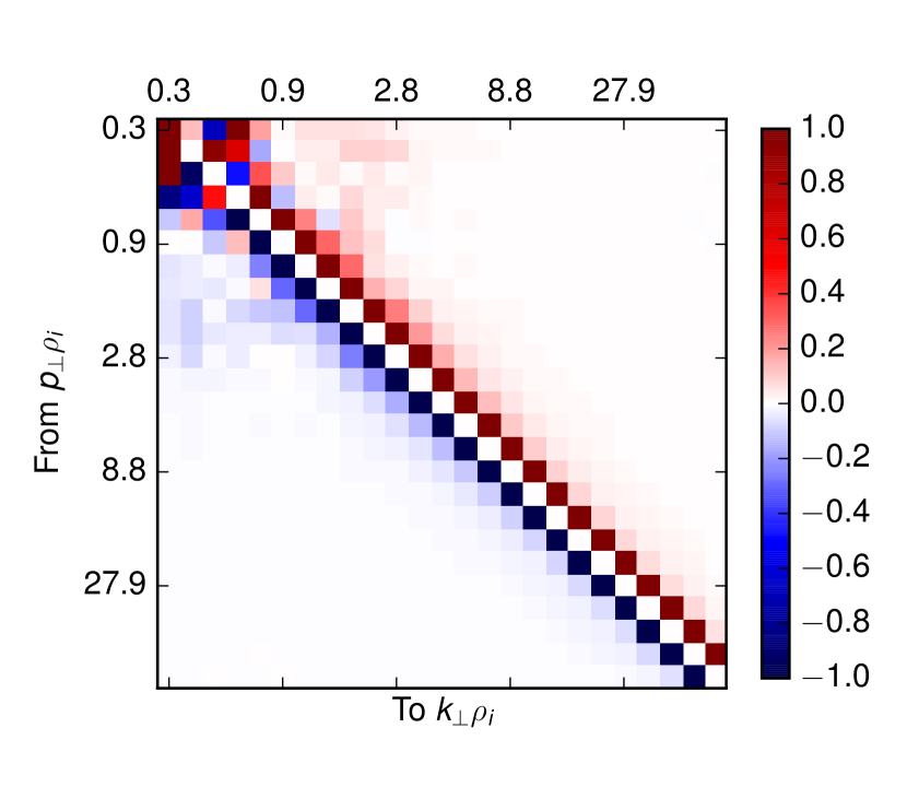
Figure 2: Nonlinear shell-to-shell transfer function for electrons, normalized to the maximum absolute value of each wavenumber scale.

With this setup, we analyze the net nonlinear shell-to-shell energy transfer, which is obtained by summing over all $q$ wavenumbers in Eq. (2). The resulting matrix (including the symmetric terms due to the antenna, and normalized for each $k_{\perp}$ scale) is displayed for the electron species in Fig. 2. Numerical inspection shows that the antenna source acts almost exclusively on the lowest shell, and diminishes very quickly for higher shell numbers. Studying the conservative transfer more closely, one can observe that in the range $k_{\perp}\rho_{i}\lesssim 3$, while local energy transfer dominates, there are some nonlocal contributions connecting disparate $k_{\perp}$ scales. In the range $k_{\perp}\rho_{i}>3$, on the other hand, the nonlinear transfer is quite local $\left(k_{\perp}\approx p_{\perp}\right)$, i.e. dominated by direct energy transfer between neighboring shells.

Nonlocal mediation. Beyond the net energy transfer, we now extend the analysis to differentiate between different mediators, i.e. $q$ wavenumbers. To this end, we evaluate the transfer function of Eq. (2) with triply filtered inputs, i.e., with fields and distributions condensed into shells $K,P,Q$. Even with the limited number of wavenumber shells used here, this diagnostic is extremely expensive (approximately $\propto N^{2}$, or about 150,000 core-hours here), and is thus only evaluated instantaneously for a single timestep. Its results can be visualized in a compact way, e.g., by means of Kraichnan’s locality functions (Kraichnan, 1959). The so-called infrared (IR) locality function is defined (following the notation of Ref. (Teaca et al., 2012)) as

$$\Pi(k_{p}|k_{c})=\sum_{K=c+1}^{N}\left[\sum_{P=1}^{N}\sum_{Q=1}^{p}+\sum_{P=1}^{p}\sum_{Q=p+1}^{N}\right]T_{K,P,Q}$$

and retains, for a fixed shell $k_{c}$ with a varying ’probe’ wavenumber $k_{p}$, only transfers for which at least one leg $p$ or $q$ is smaller than $k_{p}$. Thus, starting with $k_{p}=k_{c}$ (retaining all transfers) and then moving the probe $k_{p}$ away from $k_{c}$, the most local transfers are successively removed. For an extensive description of this setup, we refer the reader to Sec. V of Ref. (Teaca et al., 2014).

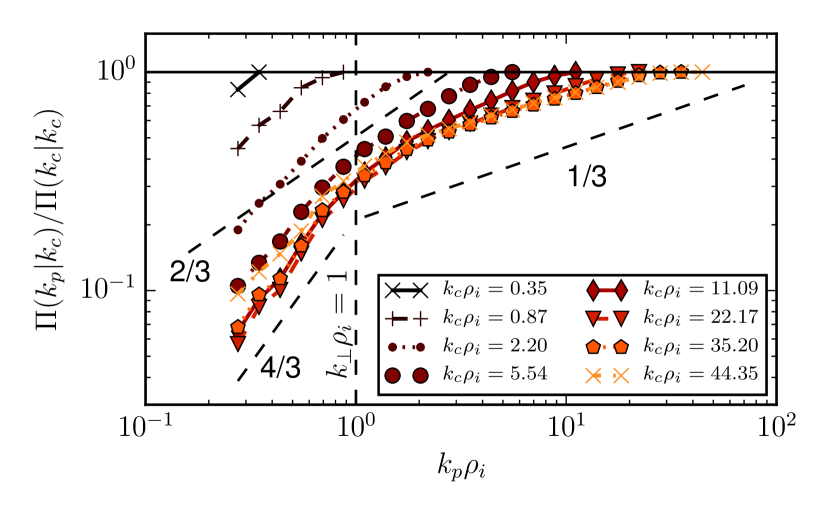
Figure 3: Infrared locality functions for several shells $k_{c}$, normalized to the total nonlinear energy transfer through $k_{c}$, versus the probe wavenumber $k_{p}\rho_{i}$. For the curves with $k_{c}\rho_{i}\gtrsim 5$, a change in slope is apparent when the probe $k_{p}$ crosses the ion gyroradius scale.

For several $k_{c}$ shells, we show the corresponding IR locality functions $\Pi\left(k_{p}|k_{c}\right)/\Pi\left(k_{c}|k_{c}\right)$ in Fig. 3. By plotting the curves versus the probe wavenumber $k_{p}$ instead of the conventional ratio $k_{p}/k_{c}$, Fig. 3 highlights the existence of a meaningful physical scale length at $k_{\perp}\rho_{i}\sim 1$, indicating a lack of self-similarity. Indeed, the locality function curves for $k_{c}\rho_{i}\gtrsim 5$ exhibit a transition in their slope that occurs close to the ion gyroradius scale, $k_{p}\rho_{i}\sim 1$: for $k_{p}\rho_{i}>1$ the nonlinear energy transfer is rather nonlocal, with a locality exponent between 2/3 and 1/3; for $k_{p}\rho_{i}<1$, a more local exponent of 4/3, as in Navier-Stokes turbulence (Kraichnan, 1966), is found. As a consequence of this property, for $5\lesssim k_{c}\lesssim 51.2$, nonlocal transfers mediated by fluctuations in the tail of the MHD range at $k_{p}\rho_{i}\lesssim 1$ are responsible for at least 30% of the total energy transfer through these shells. Note that this does not contradict the above observation that the net nonlinear transfer for large $k_{\perp}$ is local. Indeed, the nonlinear triad $\boldsymbol{k}+\boldsymbol{p}+\boldsymbol{q}=0$ for such nonlocal interactions is characterized by $\left|\boldsymbol{q}\right|\ll\left|\boldsymbol{k}\right|,\left|\boldsymbol{p}\right|$ and thus $\left|\boldsymbol{k}\right|\approx\left|\boldsymbol{p}\right|$, consistent with a local net transfer between $\boldsymbol{k}$ and $\boldsymbol{p}$. Finally, we note that while all of the above statements were illustrated with results for the electron species, the nonlinear ion energy transfer (not shown) exhibits the same characteristics, though with an even more pronounced nonlocality (exponent $\sim 1/12$), and at least 50% of the transfer mediated by modes in the tail of the MHD range.

Collisional dissipation. Next, we study the spectral properties of the collisional dissipation rate by measuring the contribution of the collision term to the free energy balance. The resulting graphs are presented in Fig. 4 for both electron and ion species, as well as their sum. About 70% of the total dissipation is found to arise from electron collisions, which exhibit a broad peak around $k_{\perp}\rho_{i}\sim 1-5$. Qualitatively, this peak is consistent with electron Landau damping acting on the magnetic energy spectrum shown in Figure 1. Despite peaking at these relatively small $k_{\perp}$ wavenumbers, electron dissipation remains strong throughout the spectrum, and begins to intensify somewhat at $k_{\perp}\rho_{i}\gtrsim 30$. At $k_{\perp}\rho_{i}\sim 1$, where ion transit-time damping is expected to transfer field energy to ion particle energy, there is in fact little ion heating. At these scales the ion free energy (not shown) is comparable to the magnetic fluctuation energy, but it is cascaded to smaller scales in both position and velocity space, and is dissipated close to the electron gyroradius scale (around $k_{\perp}\rho_{i}\sim 25$). This observation is consistent with an ion entropy cascade and the fact that $\nu_{i}\ll\nu_{e}$ (Schekochihin et al., 2009; Tatsuno et al., 2009; Howes et al., 2011a). Taking into account both species’ contributions, we find an essentially flat dissipation spectrum throughout the kinetic wavenumber range, contrasting with some interpretations of solar wind data (Alexandrova et al., 2009; Sahraoui et al., 2009) which suggested that the electron gyroradius scale acts as the dominant dissipation scale.

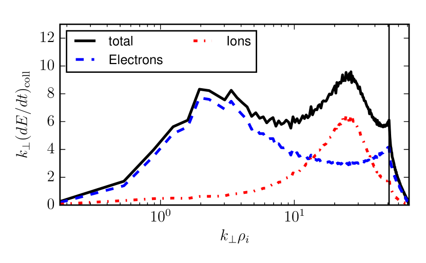
Figure 4: Normalized, short-time averaged collisional dissipation for electrons, ions, and its total value. Curves are multiplied by $k_{\perp}$ so the area under the curve is proportional to the energy dissipation rate.

Conclusions. In the present study, the first gyrokinetic simulation of kinetic Alfvén wave turbulence coupling all scales from the tail of the MHD range to the electron gyroradius scale was performed, with the goal of analyzing fundamental properties of nonlinear energy transfer and collisional dissipation for parameters relevant to the solar wind. It was found that nonlinear energy transfer in the kinetic range, particularly for $k_{\perp}\rho_{i}\gtrsim 5$, is considerably more nonlocal than hydrodynamic turbulence, as suggested by previous theoretical considerations (Howes et al., 2011b), and is to a significant percentage ($>$30%) mediated by the tail of the MHD cascade just below $k_{\perp}\rho_{i}\sim 1$, while the net energy transfer occurs mainly between nearest-neighbor shells. For $T_{e}/T_{i}=1$ and $\beta_{i}=1$, similar to the near-Earth solar wind, 70% of the injected energy is dissipated through the electron species, whose dissipation spectrum peaks around $k_{\perp}\rho_{i}\sim 1-5$, consistent with electron Landau damping. The ion free energy, on the other hand, is cascaded to small scales and dissipated around $k_{\perp}\rho_{i}\sim 25$. These findings underscore the presence of strong dissipation throughout the kinetic range $k_{\perp}\rho_{i}\gtrsim 1$, justifying the common notion of a ’dissipation range’, and demonstrating a coupling across multiple scales of both transfer and dissipation.

Acknowledgments. The authors acknowledge fruitful discussions with F. Muller, A. Bañón Navarro and M.J. Pueschel. The research leading to these results has received funding from the European Research Council under the European Union’s Seventh Framework Programme (FP7/2007-2013)/ERC Grant Agreement No. 277870, NSF CAREER Award AGS-1054061, and U.S. DOE Award No. DEFG0293ER54197. Furthermore, this work was facilitated by the Max-Planck/Princeton Center for Plasma Physics. The Rechenzentrum Garching (RZG) is gratefully acknowledged for providing computational resources used for this study. Parts of this research also profited from resources of the National Energy Research Scientific Computing Center, a DOE Office of Science User Facility supported by the Office of Science of the U.S. Department of Energy under Contract No. DE-AC02-05CH11231.

References

- Richardson and Smith (2003) J. D. Richardson and C. W. Smith, Geophys. Res. Lett. 30, 1206 (2003).
- Bruno and Carbone (2013) R. Bruno and V. Carbone, Living Rev. Sol. Phys. 10, 2 (2013).
- Bale et al. (2005) S. D. Bale, P. J. Kellogg, F. S. Mozer, T. S. Horbury, and H. Reme, Phys. Rev. Lett. 94, 215002 (2005), physics/0503103 .
- Alexandrova et al. (2009) O. Alexandrova, J. Saur, C. Lacombe, A. Mangeney, J. Mitchell, S. J. Schwartz, and P. Robert, Phys. Rev. Lett. 103, 165003 (2009), arXiv:0906.3236 [physics.plasm-ph] .
- Sahraoui et al. (2009) F. Sahraoui, M. L. Goldstein, P. Robert, and Y. V. Khotyaintsev, Phys. Rev. Lett. 102, 231102 (2009).
- Sahraoui et al. (2010) F. Sahraoui, M. L. Goldstein, G. Belmont, P. Canu, and L. Rezeau, Phys. Rev. Lett. 105, 131101 (2010).
- Chen et al. (2013) C. H. K. Chen, S. Boldyrev, Q. Xia, and J. C. Perez, Phys. Rev. Lett. 110, 225002 (2013), arXiv:1305.2950 [physics.space-ph] .
- Howes et al. (2008) G. G. Howes, W. Dorland, S. C. Cowley, G. W. Hammett, E. Quataert, A. A. Schekochihin, and T. Tatsuno, Phys. Rev. Lett. 100, 065004 (2008), arXiv:0711.4355 .
- Howes et al. (2011a) G. G. Howes, J. M. TenBarge, W. Dorland, E. Quataert, A. A. Schekochihin, R. Numata, and T. Tatsuno, Phys. Rev. Lett. 107, 035004 (2011a), arXiv:1104.0877 [astro-ph.SR] .
- Wan et al. (2012) M. Wan, W. H. Matthaeus, H. Karimabadi, V. Roytershteyn, M. Shay, P. Wu, W. Daughton, B. Loring, and S. C. Chapman, Phys. Rev. Lett. 109, 195001 (2012).
- Salem et al. (2012) C. S. Salem, G. G. Howes, D. Sundkvist, S. D. Bale, C. C. Chaston, C. H. K. Chen, and F. S. Mozer, Astrophys. J. Lett. 745, L9 (2012).
- TenBarge et al. (2013) J. M. TenBarge, G. G. Howes, and W. Dorland, Astrophys. J. 774, 139 (2013).
- TenBarge and Howes (2013) J. M. TenBarge and G. G. Howes, Astrophys. J. Lett. 771, L27 (2013), arXiv:1304.2958 [physics.plasm-ph] .
- Osman et al. (2014) K. T. Osman, W. H. Matthaeus, J. T. Gosling, A. Greco, S. Servidio, B. Hnat, S. C. Chapman, and T. D. Phan, Phys. Rev. Lett. 112, 215002 (2014), arXiv:1403.4590 [physics.space-ph] .
- Brizard and Hahm (2007) A. J. Brizard and T. S. Hahm, Rev. Mod. Phys. 79, 421 (2007).
- Podesta (2013) J. J. Podesta, Sol. Phys. 286, 529 (2013).
- Jenko et al. (2000) F. Jenko, W. Dorland, M. Kotschenreuther, and B. N. Rogers, Phys. Plasmas. 7, 1904 (2000).
- TenBarge et al. (2014) J. M. TenBarge, G. G. Howes, W. Dorland, and G. W. Hammett, Comput. Phys. Commun. 185, 578 (2014), arXiv:1305.2212 [physics.plasm-ph] .
- Schekochihin et al. (2009) A. A. Schekochihin, S. C. Cowley, W. Dorland, G. W. Hammett, G. G. Howes, E. Quataert, and T. Tatsuno, Astrophys. J. Suppl. Ser. 182, 310 (2009), arXiv:0704.0044 .
- Bañón Navarro et al. (2011a) A. Bañón Navarro, P. Morel, M. Albrecht-Marc, D. Carati, F. Merz, T. Görler, and F. Jenko, Phys. Rev. Lett. 106, 055001 (2011a), arXiv:1008.3974 [physics.plasm-ph] .
- Bañón Navarro et al. (2011b) A. Bañón Navarro, P. Morel, M. Albrecht-Marc, D. Carati, F. Merz, T. Görler, and F. Jenko, Phys. Plasmas. 18, 092303 (2011b).
- Teaca et al. (2012) B. Teaca, A. B. Navarro, F. Jenko, S. Brunner, and L. Villard, Phys. Rev. Lett. 109, 235003 (2012).
- Teaca et al. (2014) B. Teaca, A. B. Navarro, and F. Jenko, Phys. Plasmas. 21, 072308 (2014), arXiv:1404.2080 [physics.plasm-ph] .
- Goldreich and Sridhar (1995) P. Goldreich and S. Sridhar, Astrophys. J. 438, 763 (1995).
- Sahraoui et al. (2013) F. Sahraoui, S. Y. Huang, G. Belmont, M. L. Goldstein, A. Rétino, P. Robert, and J. D. Patoul, Astrophys. J. 777, 15 (2013).
- Kraichnan (1959) R. H. Kraichnan, J. Fluid Mech. 5, 497 (1959).
- Kraichnan (1966) R. H. Kraichnan, Phys. Fluids 9, 1728 (1966).
- Tatsuno et al. (2009) T. Tatsuno, W. Dorland, A. A. Schekochihin, G. G. Plunk, M. Barnes, S. C. Cowley, and G. G. Howes, Phys. Rev. Lett. 103, 015003 (2009), arXiv:0811.2538 [physics.plasm-ph] .
- Howes et al. (2011b) G. G. Howes, J. M. TenBarge, and W. Dorland, Phys. Plasmas. 18, 102305 (2011b), arXiv:1109.4158 [astro-ph.SR] .