Optimal Morse functions and $H(\mathcal{M}^{2},\mathbb{A})$ in $\tilde{O}(N)$ time

Abstract

In this work, we design a nearly linear time discrete Morse theory based algorithm for computing homology groups of 2-manifolds, thereby establishing the fact that computing homology groups of 2-manifolds is remarkably easy. Unlike previous algorithms of similar flavor, our method works with coefficients from arbitrary abelian groups. Another advantage of our method lies in the fact that our algorithm actually elucidates the topological reason that makes computation on 2-manifolds easy. This is made possible owing to a new simple homotopy based construct that is referred to as expansion frames. To being with we obtain an optimal discrete gradient vector field using expansion frames. This is followed by a pseudo-linear time dynamic programming based computation of discrete Morse boundary operator. The efficient design of optimal gradient vector field followed by fast computation of boundary operator affords us near linearity in computation of homology groups.
Moreover, we define a new criterion for nearly optimal Morse functions called pseudo-optimality. A Morse function is pseudo-optimal if we can obtain an optimal Morse function from it, simply by means of critical cell cancellations. Using expansion frames, we establish the surprising fact that an arbitrary discrete Morse function on 2-manifolds is pseudo-optimal.

Classical Morse Theory [16, 17] analyzes the topology of the Riemannian manifolds by studying critical points of smooth functions defined on it. In the 90’s Robin Forman formulated a completely combinatorial analogue of Morse theory, now known as discrete Morse theory. The fact that Forman’s theory can be formulated in language of graph theory makes it possible to use powerful machinery from modern algorithmics to provide efficient algorithms with rigorous guarantees. It is worth noting that the reader can understand this work without any prior knowledge of Morse theory as long as he understands the equivalent graph theory problem. Knowledge of discrete Morse theory is however useful for the more inclined reader who wishes to understand the context and wider range of applicability of this work. In subsection 1.2, we provide a quick overview of the graph theory setting of discrete Morse theory in order to enable the reader to make a quick foray into the core computer science problem at hand.

1 Background and Preliminaries

1.1 Discrete Morse theory

Forman provides an extremely readable introduction to discrete Morse theory in [7].

Notation 1.

The relation ’$\prec$’ is used to denote the following: $\tau\prec\sigma\rightarrow\tau\subset\sigma\,\,\&\,\dim\,\tau=\dim\sigma-1$.

Notation 2 (The d-(d-1) level of Hasse graph).

By the term, d-(d-1) level of Hasse graph $\mathcal{H}$ we mean the subset of edges of the Hasse graph that join d-dimensional cofaces to (d-1)-dimensional faces of Hasse graph.

Definition 3.

Boundary & Couboundary of a simplex $\sigma$: We define the boundary and respectively coboundary of a simplex as $bd\>\sigma\,=\>\{\tau\,|\,\tau\prec\sigma\}$ $cbd\>\sigma=\{\rho\,|\,\sigma\prec\rho\}$

Definition 4.

Discrete Morse Function: Let $\mathcal{K}$ denote a finite regular cell complex and let $\mathcal{L}$ denote the set of cells of $\mathcal{K}$. A function $\mathcal{F}:\mathcal{L}\rightarrow\mathbb{R}$ is called a discrete Morse function (DMF) if it usually assigns higher values to higher dimensional cells, with at most one exception locally at each cell. Equivalently, a function $\mathcal{F}:\mathcal{L}\rightarrow\mathbb{R}$ is a discrete Morse function if for every $\sigma^{m}\in\mathcal{L}$ we have:
(A.)  $\mathcal{N}_{1}(\sigma)=\#\{\rho\in cbd\>\sigma|\mathcal{F}(\rho)\leq\mathcal{F}(\sigma)\}\leq 1$
(B.)  $\mathcal{N}_{2}(\sigma)=\#\{\tau\in bd\>\sigma\>\>|\mathcal{F}(\tau)\geq\mathcal{F}(\sigma)\}\leq 1$
A cell $\sigma$ is critical if $\mathcal{N}_{1}(\sigma)=\mathcal{N}_{2}(\sigma)=0$; A non-critical cell is a regular cell.

Definition 5 (Combinatorial Vector Field).

A combinatorial vector field (DVF) $\mathcal{V}$ on $\mathcal{L}$ is a collection of pairs of cells $\{\langle\alpha,\beta\rangle\}$ such that $\{\alpha^{m}\prec\beta^{(m+1)}\}$ and each cell occurs in at most one such pair of $\mathcal{V}$.

Definition 6 (Discrete Gradient Vector Field).

A pair of cells $\{\alpha^{m}\prec\beta^{(m+1)}\}$ s.t. $\mathcal{F}(\alpha)\geq\mathcal{F}(\beta)$ determines a gradient pair. A discrete gradient vector field (DGVF) $\mathcal{V}$ corresponding to a DMF $\mathcal{F}$ is a collection of cell pairs ${\alpha^{(p)}\prec\beta^{(p+1)}}$ such that ${\alpha^{(p)}\prec\beta^{(p+1)}}\in\mathcal{V}$ iff $\mathcal{F}(\beta)\leq\mathcal{F}(\alpha)$.

Definition 7.

We define $\mathcal{V}$-path to be a cell sequence $\sigma_{0}^{(m)}$, $\tau_{0}^{(m+1)}$, $\sigma_{1}^{(m)}$, $\tau_{1}^{(m+1)}$, $\ldots\sigma_{q}^{(m)}$, $\tau_{q}^{(m+1)}$, $\sigma_{q+1}^{(m)}$ s.t. for $i=0,\ldots q,\{\sigma_{i}\prec\tau_{i}\}\in\mathcal{V}$, $\sigma_{i}\prec\tau_{i}\succ\sigma_{i+1}$ and $\sigma_{i}\neq\sigma_{i+1}$. The $\mathcal{V}$-path corresponding to a DMF $\mathcal{F}$ is a gradient path of $\mathcal{F}$.

Theorem 8 (Forman [6]).

Let $\mathcal{K}$ be a CW Complex with a DMF $\mathcal{F}$ defined on it. Then $\mathcal{K}$ is homotopy equivalent to a CW complex $\Omega$, such that $\Omega$ has precisely one m-dimensional cell for every m-dimensional critical cell in $\mathcal{K}$ and no other cells besides these. Moreover, let $c_{m}$ be the number of m-dimensional critical cells, $\beta_{m}$ the $m^{th}$ Betti Number w.r.t. some vector field $\mathcal{V}$ and $n$ the maximum dimension of $\mathcal{K}$. Then we have:
The Weak Morse Inequalities:

$$(\textsf{A}.) \;\textrm{For every }m\in\{0\ldots n\}\textrm{: we have }c_{m}\geq\beta_{m}.$$ (1)

$$(\textsf{B}.) \;c_{0}-c_{1}\ldots+(-1)^{n}c_{n}=\beta_{0}-\beta_{1}\ldots+(-1)^{n}\beta_{n}=\chi(\mathcal{K})$$ (2)

The Strong Morse Inequalities:

$$\textrm{For every }m\in[0,n]:c_{m}-c_{m-1}\ldots+(-1)^{m}c_{0}\geq\beta_{m}-\beta_{m-1}\ldots+(-1)^{m}\beta_{0}$$ (3)

Notation 9.

We shall denote the sum of Betti numbers by the symbol $\varLambda$ and sum of number of critical cells by symbol $\varUpsilon$. In other words,

$$\varLambda\stackrel{{\scriptstyle\text{def}}}{{=}}\sum\limits_{i=0}^{n}\beta_{i}\quad\quad\varUpsilon\stackrel{{\scriptstyle\text{def}}}{{=}}\sum\limits_{i=0}^{n}c_{i}$$

.

Notation 10.

The symbol $\tilde{O}(n)$ is used to indicate nearly linear. It is given by $\tilde{O}(n)=n\left(\log n\right)^{O(1)}$.

Given a DGVF, we can use topological sort to obtain a total order on the cells and then assign (arbitrary) ascending function values to the sorted list of cells. This will give us a Morse function that agrees with the partial order imposed by the gradient vector field. Any such Morse function will have the same critical cells as the gradient vector field. Hence, we shall use the terms optimal Morse function and optimal gradient vector field interchangeably.

Definition 11 (WMOC).

Let $\varUpsilon(\mathcal{M})$ denote the sum of Morse numbers across all dimensions for the optimal DGVF on $\mathcal{M}$. We say that a family of simplicial complexes $\varOmega$ satisfies the weak Morse optimality condition (WMOC) when $\forall\mathcal{M}\in\varOmega$, $\varUpsilon(\mathcal{M})=\tilde{O}(1)$. In other words, $\varUpsilon(\mathcal{M})\ll|\mathcal{M}|$ uniformly $\forall\mathcal{M}\in\varOmega$.

1.2 Graph Theoretic Reformulation

Given a simplicial complex $\mathcal{K}$, we construct its Hasse Graph representation $\mathcal{H_{\mathcal{K}}}$ (an undirected, multipartite graph) as follows: To every simplex $\sigma_{\mathcal{K}}^{d}\in\mathcal{K}$ associate a vertex $\sigma_{\mathcal{H}}^{d}\in\mathcal{H_{\mathcal{K}}}$. The dimension d of the simplex $\sigma_{\mathcal{K}}^{d}$ determines the vertex level of the vertex $\sigma_{\mathcal{H}}^{d}$ in $\mathcal{H_{\mathcal{K}}}$. Every face incidence $(\tau_{\mathcal{K}}^{d-1},\sigma_{\mathcal{K}}^{d})$ determines an undirected edge $\langle\tau_{\mathcal{H}}^{d-1},\sigma_{\mathcal{H}}^{d}\rangle$ in $\mathcal{H_{\mathcal{K}}}$. Now orient the graph $\mathcal{H_{\mathcal{K}}}$ to a form a new directed graph $\mathcal{\overline{H_{\mathcal{K}}}}$. Initally all edges of $\mathcal{\overline{H}_{\mathcal{K}}}$ have default orientation. The default orientation is a directed edge $\sigma_{\mathcal{H}}^{d}\rightarrow\tau_{\mathcal{H}}^{d-1}\in\mathcal{\overline{H_{\mathcal{K}}}}$ that connects a k-dim node $\sigma_{\mathcal{H}}^{d}$ to a (k-1)-dim node $\tau_{\mathcal{H}}^{d-1}$. Finally, associate a matching $\mathcal{M}$ to graph $\mathcal{H_{\mathcal{K}}}$. If an edge $\langle\tau_{\mathcal{H}}^{d-1},\sigma_{\mathcal{H}}^{d}\rangle\in\mathcal{M}$ then, reverse the orientation of that edge to $\tau_{\mathcal{H}}^{d-1}\rightarrow\sigma_{\mathcal{H}}^{d}\in\mathcal{\overline{H}_{\mathcal{K}}}$. The matching induced reorientation needs to be such that the graph $\overline{\mathcal{H}_{\mathcal{K}}}$ is a Directed Acyclic Graph. A graph matching on $\mathcal{H_{\mathcal{K}}}$ that leaves the graph $\overline{\mathcal{H_{\mathcal{K}}}}$ acyclic in the manner prescribed above is known as Morse Matching. Table 1 provides a translating dictionary from simplicial complexes to their Hasse graphs. See Table 1.

Figure 1: Matching induced orientation of Hasse Graph

Table 1: Graph Theoretic dictionary for Morse Matching

	Morse theory on Cell Complex $\mathcal{K}$	Graph theory on Hasse Graph $\overline{\mathcal{H}_{\mathcal{K}}}$
1.	gradient Pair $\langle\alpha^{d-1},\beta^{d}\rangle\in\mathbb{V}$	Matched pair of vertices $(\alpha,\beta)\in\mathcal{H_{\mathcal{K}}}$
2.	Dimension d	Multipartite Graph Level d
3.	$\sigma^{d-1}\prec\tau^{d}$ s.t. $\langle\sigma^{d-1},\tau^{d}\rangle\mathcal{\notin\mathbb{V}}$	Default down-edge $\tau\rightarrow\sigma$
4.	$\sigma^{d-1}\prec\tau^{d}$ s.t. $\langle\sigma^{d-1},\tau^{d}\rangle\mathcal{\in\mathbb{V}}$	Matching up-edge $\sigma\rightarrow\tau$
5.	$\mathbb{V}$-Path	Directed Path
6.	Non-trivial Closed $\mathbb{V}$-Path	Directed Cycle
7.	CVF	Matching on the Hasse Graph
8.	DGVF	Morse Matching (i.e. Acyclic Matching)
9.	Critical Cell $\zeta^{d}$	Unmatched Vertex $\zeta$
10.	Regular Cell $\xi^{d}$	Matched Vertex $\xi$

1.3 Prior Work

Joswig et al. [10] proved the NP-completess of the decision problem and posed the approximability of optimality of Morse gradient vector fields (for general dimensional complexes) as an open problem, by pointing out an error in Lewiner’s claim about inapproximability in [13]. Recently [18] provided an $O(\log^{2}n)$ factor $\tilde{O}(n)$ time approximation algorithm for the optimal discrete gradient vector field (that minimizes the number of critical cells). Recently, Burton et al. [5] developed an FPT algorithm for optimizing Morse functions. Some of the notable works that seek optimality of Morse matchings by applying heuristics in general are [1, 2, 8, 9, 10, 15, 4]. The works that constitute more relevant prior work for us are those that achieve optimality by restricting the problem to 2-manifolds in nearly linear time [11, 14] and quadratic time [3] respectively. Ours is however the first algorithm to compute homology groups of 2-manifolds with arbitrary coefficients in nearly linear time.

2 Boundary Operator Computation

The analytic formula for boundary operator is given in Forman[6]. The obvious interpretation of the formula gives an exponential time algorithm. We give an efficient $O(\kappa n)$ time algorithm where $\kappa$ is the total number of critical cells which is nearly-linear if the number of topologically interesting features are small relative to the number of simplices. Hence, we have a pseudolinear time complexity algorithm for boundary operator Computation. We note of the following Theorem from Forman[6]:

Theorem 12 (Boundary Operator Computation. Forman [6]).

Consider an oriented simplicial complex. Then for any critical (p+1)-simplex $\beta$ set:

$$\triangle\beta=\sum\limits_{critical\>\alpha(p)}\>P_{\alpha\beta}\>\alpha$$

$$P_{\alpha\beta}=\sum\limits_{\gamma\in\Gamma(\beta,\alpha)}\varTheta(\gamma)$$

where $\Gamma(\beta,\alpha)$ is the set of discrete gradient paths which go from a face in the boundary of $\beta$ to $\alpha$ The multiplicity $\varTheta(\gamma)$ of any gradient path $\gamma$ is equal to $\pm 1$ depending on whether given $\gamma$ the orientation on $\beta$ induces the chosen orientation on $\alpha$ or the opposite orientation. The formula for the boundary operator above computes the homology of complex K.

We observe that we need ’formal sums’ of critical cells at each critical cell. However, there is an advantage in calculating these formal sums for intermediate regular cells as well since this can potentially speedup calculations at critical cells. Since topological sort also does ordering for us, we can start at the lowest valued critical cell. We proceed to the next higher valued cell and observe that we have two cases.

Also, we assume that our complex has a pre-assigned orientation. The angular brackets $<,>$ in the formulae above denote the pre-assigned orientation. Once the boundary operator is ready we use Smith normal form algorithm over a collapsed complex that is provably significantly smaller than the original complex, in a mathematically precise sense.

Let us denote by $\triangle\sigma$ the boundary operator computation for cell $\sigma^{m}.$ We now make an inductive hypothesis that the computation of the $\triangle$ operator has been done for all the maximal faces / single coface (since they are all lower valued Morse cells). Then the value of the $\triangle$ operator for the new cell is calculated as follows:

Case 1: All flow emanating from a cell goes out through its boundary faces. No lower-valued co-faces.

$$\triangle\sigma=\sum_{\begin{subarray}{c}\tau_{i}\prec\sigma\\ \exists\xi\textsf{ s.t. }\langle\tau_{i},\xi\rangle\in\mathscr{V}_{m}\\ \langle\tau_{i},\sigma\rangle\notin\mathscr{V}_{m}\end{subarray}}\triangle\tau_{i}\times<\partial\sigma,\tau_{i}>+\sum_{\begin{subarray}{c}\bm{\alpha_{j}}\prec\sigma\\ \cancel{\exists}\xi\textsf{ s.t. }\langle\bm{\alpha_{j}},\xi\rangle\in\mathscr{V}_{m}\\ \cancel{\exists}\zeta\textsf{ s.t. }\langle\zeta,\bm{\alpha_{j}}\rangle\in\mathscr{V}_{m-1}\end{subarray}}\bm{\alpha_{j}}\times\langle\partial\sigma,\bm{\alpha_{j}}\rangle$$ (4)

The first formula takes care of Case 1 where flow goes out through the faces of the boundary. Note that in the formula above, $\tau^{m-1}$ is a placeholder for non-critical faces (if any) of $\sigma^{m}$, i.e. $\{\tau^{m-1}\prec\sigma^{m}\}$, which are not a part of the Discrete Gradient vector field which is equivalent to saying $f(\tau)<f(\sigma)$. Similarly, $\alpha^{m-1}$ is a representative for the critical faces (if any) of$\sigma^{m}.$ This formula holds irrespective of whether $\sigma^{m}$ itself is critical or non-critical. In case of computation of boundary of a critical $\sigma^{m}$ such that $m=0$, i.e. when $\sigma^{m}$ is a critical point, the boundary is null.

Case 2: The cell has $1$ lower valued coface.

$$\triangle\sigma=<\partial\beta,\sigma>\times\triangle\beta$$ (5)

The second formula takes care of Case 2 when $\sigma^{m}$ has a lower valued co-face $\beta^{m+1}$.

Case 3: The 0-dimensional cell $\sigma$ is the unique minima.

$$\triangle\sigma=\emptyset$$ (6)

Theorem 13 (Boundary Operator Computation: Correctness Proof).

The Algorithm correctly computes boundary operator $\triangle$.

Proof.

Note that, to begin with we start with a list of cells in an ascending total order. Let us call this list $\mathcal{L}$. This total order is one of the total orders that is compatible with the partial order prescribed by the gradient vector field $\mathscr{V}$. If we assign the function value ’i’ i.e. the index of some cell $\mathcal{L}[i]$ to each cell in $\mathcal{L}$, we essentially obtain a Morse function compatible with the gradient vector field. The first cell we process is one with the lowest function value (i.e. the unique minima). This cell is then followed by cells with increasingly higher Morse function values. To prove that the formulaic computation of the $\triangle$ operator as expressed in subroutine calcBdryOp() is, in fact, the same as expressed in Theorem 12 we proceed by induction. Let $\sigma_{1}$ denote the unique minima. The base case of induction for $\triangle\sigma_{1}$ is trivial. Now suppose that for all cells in the set $\{\sigma_{1},\sigma_{2},\ldots\sigma_{I}\}$, we have correctly computed the boundary operator as prescribed in Theorem 12. Now suppose we encounter cell $\sigma_{I+1}$. Suppose that $\sigma_{I+1}$ has a lower valued coface $\beta$ i.e. ($\sigma_{I+1}\prec\beta$ & $\langle\sigma_{I+1},\beta\rangle\in\mathscr{V}$). Since $\beta$ has lower function value as compared to $\sigma_{I+1}$ (by hypothesis), we conclude that $\beta=\sigma_{J+1}$ for some $J<I$. All paths emanating from $\sigma_{I+1}$ must go through $\beta$. The orientation induced by some path $\gamma_{i}$ $\beta\overset{\gamma_{i}}{\rightsquigarrow}\rho$ from $\beta$ to some critical cell say $\rho$ is $\iota$ where $\iota=\pm 1$, then the orientation of path $\sigma_{I+1}\mathrel{\leavevmode\hbox to22.01pt{\vbox to11.63pt{\text{[drawing]}}}}\rho$ will be $\langle\partial\beta,\sigma_{I+1}\rangle\times\iota$. Therefore, the total count of paths (with induced orientation accounted for) will be $\langle\partial\beta,\sigma\rangle\times\triangle\beta$. Hence, the boundary operator computation done in $\textbf{calcBdryOp}()$ is valid for the case when $\sigma_{I+1}$ has a lower valued coface.
Finally, assume that $\sigma_{I+1}$ does not have any lower valued coface. Therefore, the flow leaving from $\sigma_{I+1}$ will be through each of its faces (except possibly one higher valued face). If it indeed has a (matched) higher valued face then flow will be entering it through that face and hence the face in question isn’t relevant in calculating the weighted sum of gradient paths that leave $\sigma_{I+1}$. When consider lower valued faces of $\sigma_{I+1}$, we make a distinction between faces that are non-critical and those those that are critical. If a face say $\bm{\alpha_{j}}$ is critical, then clearly we are justified in directly including the entry $\bm{\alpha_{j}}\times\langle\partial\sigma,\bm{\alpha_{j}}\rangle$ as part of our «formal sum» that makes up the cell boundary. As for the non-critical entries of the formula, namely $[\triangle\tau_{i}\times<\partial\sigma,\tau_{i}>]$, we impose an additional constraint $\langle\tau_{i},\xi\rangle\in\mathscr{V}_{m}$ (as opposed to $\langle\xi,\tau_{i}\rangle\in\mathscr{V}_{m-1}$) in the summation. In doing so, we are ruling out all entries that would valid directed paths going out of $\sigma_{I+1}$ but those that won’t add up to make gradient paths as prescribed by Theorem 12. Now since $\tau_{i}$ is lower valued its boundary $\triangle\tau_{i}$ has already been calculated correctly by Induction Hypothesis. But clearly every gradient path emerging from $\sigma_{I+1}$ must first pass through one of these $\tau_{i}$’s. Also, for each of these gradient paths, the orientations will change precisely by the multiple of $\langle\tau_{i},\xi\rangle$. Therefore the weighted sum of (non-trivial) gradient paths from $\sigma_{I+1}$ will be the sum of all the contributions by boundaries of each of the non-critical faces $\tau_{i}$. To complete the argument for the induction step, we note that these sums along with contributions from the critical faces of $\sigma_{I+1}$ takes into account each gradient path precisely once. Also, it is easy to see that multiplication by co-orientation at each step provides the weights to ensure that the final entry will decide the induced orientation. Hence proved. ∎

Theorem 14 (Complexity of Computing Boundary Operator).

The complexity of computing the boundary operator is $O(\varUpsilon\times\mathcal{N})$.

Proof.

For the Hasse graph $\mathcal{H}(\mathcal{V},\mathcal{E})$ of a simplicial complex, $\mathcal{E}\leq\mathcal{V}\times\mathcal{D}$ where $\mathcal{D}$ is the maximum dimension of cells in the complex (which in our case is 2). Therefore, $|\mathcal{E}|=O(|\mathcal{V}|)$. (It is easy to show that for a cubical complexes as well, number of edges is $O(|\mathcal{V}|)$).The complexity of computing topological sort of the oriented Hasse graph is $O(|\mathcal{V}|+|\mathcal{E}|)$ which is same as $O(|\mathcal{V}|)$, assuming that our input manifold is either simplicial or cubical.
The for loop in Lines 9-22 of procedure calcBdryOp() costs at the most $O(\varLambda)$ per iteration while the total number of iterations is $O(|\mathcal{V}|)$. But since in our case, using Theorem 29, $\varLambda=\varUpsilon$, the total cost of the for loop is $O(|\mathcal{V}|\times\varUpsilon)$. Therefore, complexity of computing boundary operator is $O(|\mathcal{V}|\times\varUpsilon)=O(\mathcal{N}\times\varUpsilon)$, since the number of vertices in the Hasse graph is same as number of cells in the complex (i.e. the size of the complex namely $\mathcal{N}$). ∎

It is worth noting that in vast majority of the practical scenarios $\mathcal{N}\ggg\varUpsilon$, enough for us to assume that compared to the size of the complex, the ’topological complexity’, $\varUpsilon$ is nearly a constant. We therefore use the notation $\tilde{O}(\raisebox{-1.07639pt}{\scalebox{1.2}{$\cdot$}})$ (where $O(\varUpsilon\times\mathcal{N})=\tilde{O}(\mathcal{N})$) to indicate the nearly linear time complexity of boundary operator computation.

3 Frames of Expansion

3.1 Basic Formulation

Notation 15.

Let the set $\mathcal{B}(\alpha)$ denote the 0-dim cells (vertices) and 1-dim. cells (edges) incident on $\alpha$ if $\alpha$ is 2-dimensional and let $\mathcal{B}(\alpha)$ denote the 0-dim cells incident on $\alpha$ if $\alpha$ is 1-dimensional.

Definition 16 (Semigraph).

A semigraph is a set of vertices and edges s.t. every edge may have either one or two vertices incident on it.

Semigraphs generalize graphs in the sense that, in a graph, every edge is incident on precisely two vertices.

Definition 17 (Frame of expansion of a critical cell).

Given a critical cell $\alpha^{n}$ where ($n\geq 2$), consider the set of all cells that can be reached from $\alpha$, by following one of the gradient paths within the gradient vector field. We call this set the expansion set of critical cell $\alpha$ and denote it by $\widehat{\alpha}$. The frame of expansion of $\alpha$ is the $n-1$-dim. boundary of $\widehat{\alpha}$ along with the $n-2$ dim. cells incident on these boundary cells. We denote the frame of expansion of $\alpha$ by $\underline{\widehat{\alpha}}$.

Definition 18 (Frame of expansion of a boundary cell).

Given a regular boundary cell $\xi^{n-1}$ where ($n\geq 2$), suppose that $\langle\xi,\chi\rangle$ forms a gradient pair. Now consider the set of all cells that can be reached from $\xi$, by following one of the gradient paths within the gradient vector field. We call this set the expansion set of boundary cell $\xi$ and denote it as $\widehat{\xi}$. The frame of expansion of $\xi$ is the $n-1$-dimensional boundary of $\widehat{\xi}$. We denote it as $\underline{\widehat{\xi}}$.

[Method of addition of cells upon expansion] It must be noted that if there is an expansion along $\tau^{1}$ into cell $\varpi^{2}$, then we delete $\tau^{1}$ from the frame and the set $\mathcal{B}(\varpi\setminus\tau)$ is added into the frame.

Suppose we are given a regular 2-cell $\varpi^{2}$, s.t. the 1-cell $\tau^{1}\in\varpi^{2}$. The boundary of $\tau$ namely $\mathcal{B}(\tau)$ consists of two vertices say $\lambda^{0}$ and $\rho^{0}$. Note that within the set $\mathcal{B}(\varpi)$, there exist two non-intersecting paths that connect $\lambda$ and $\rho$. One path involves the singular edge $\tau$, the other path consists of edges belonging to the set $\mathcal{B}(\varpi\setminus\tau)$

Definition 19 (connectedness, connecting path).

Consider two cells $\sigma^{(m-1)},\tau^{(m-1)}$ in a complex $\mathcal{K}^{n}$. We say that $\sigma$ and $\tau$ are said to be Type 1 connected in complex $\mathcal{K}$ if there exists a cell sequence $\phi_{0}^{(m-1)}$, $\gamma_{0}^{(m)}$, $\phi_{1}^{(m-1)}$, $\gamma_{1}^{(m)}$, $\ldots\phi_{q}^{(m-1)}$, $\gamma_{q}^{(m)}$, $\phi_{q+1}^{(m-1)}$ s.t. for $i=0,\ldots q$, $\phi_{i}\prec\gamma_{i}\succ\phi_{i+1}$, $\phi_{0}=\sigma$, $\phi_{q+1}=\tau$ and $\phi_{i}\neq\phi_{i+1}$. This sequence of cells, $\phi_{0}^{(m-1)}\ldots\phi_{q+1}^{(m-1)}$ is known as a connecting path. Analogously, we say that $\sigma^{m}$ and $\tau^{m}$ are Type 2 connected in complex $\mathcal{K}^{n}$ if there exists a cell sequence $\gamma_{0}^{(m)}$, $\phi_{0}^{(m-1)}$, $\gamma_{1}^{(m)}$, $\phi_{1}^{(m-1)}$, $\ldots\gamma_{q}^{(m)}$, $\phi_{q}^{(m-1)}$, $\gamma_{q+1}^{(m)}$ s.t. for $i=0,\ldots q$, $\gamma_{i}\succ\phi_{i}\prec\gamma_{i+1}$, $\gamma_{0}=\sigma$, $\gamma_{q+1}=\tau$ and $\gamma_{i}\neq\gamma_{i+1}$. The sequence of cells, $\gamma_{0}^{(m)}\ldots\gamma_{q+1}^{(m)}$ is known as a connecting path. Finally, we say that, $\sigma^{m}$ and $\tau^{(m-1)}$ are Type 3 connected if there exists a cell $\eta^{(m-1)}\prec\sigma^{m}$ with Type 2 connectedness between $\eta$ and $\tau$.

Finally, we say that a set of $m-1$ and $m$ dim. cells are said to form a connected set if for any pair of $m-1$ dim. cells (alternatively, for any pair of $m$ dim. cells) we can find sequence of connecting cells as prescribed above.

3.2 Pseudocode for $\tilde{O}(n)$-Time Algorithm for Computing Homology of 2-manifolds

Notation 20.

Given manifold $\mathcal{M}$, we use the notation $\mathcal{M}^{d}$ to denote the d-dimensional cells of manifold $\mathcal{M}$.

Definition 21 (Boundary faces, Coboundary faces).

Given a complex $\mathcal{K}$, if there exists a cell $\vartheta^{d}$ of dimension $d$ s.t. there exists a unique $(d+1)$-dimensional cell $\varpi^{(d+1)}$ satisfying $\vartheta\prec\varpi$, then we call $\vartheta$ a d-dimensional boundary face of complex $\mathcal{K}$. Also, in this case, $\varpi$ is known as a $(d+1)$-dimensional coboundary face of complex $\mathcal{K}$.

Definition 22 (Boundary and Coboundary).

Given a complex $\mathcal{K}$, the list of all d-dimensional boundary faces of $\mathcal{K}$ is known as the d-dimensional boundary of $\mathcal{K}$. Also, list of all d-dimensional coboundary faces of $\mathcal{K}$ is known as the d-dimensional coboundary of $\mathcal{K}$.

Definition 23 ($n$-flow).

The set of gradient paths in vector field $\mathscr{V}$ on manifold $\mathfrak{M}$ that involve alternating $n$-dim. and $(n-1)$-dim. cells is known as the n-flow of $\mathscr{V}$

1:procedure calcHomology($\mathcal{M},\mathcal{A}$;)

2:   We use the mainFrame() subroutine to design a vector field $\mathscr{V}$ on $\mathcal{M}$.

3:   We then use subroutine calcBdryOp() to calculate the boundary operator $\triangle_{c}$ for DGVF $\mathscr{V}$.

4:   Finally, using chain complex implied by boundary operator $\triangle_{c}$, we calculate homology of $\mathcal{M}$ (with coefficients coming from arbitrary abelian group $\mathbb{A}$) using Smith Normal Form.

5:end procedure

6:

7:procedure calcBdryOp($\mathcal{M},\mathcal{H},\mathscr{V}$)

8:   $\textbf{topologicalSort}(\mathcal{H},\mathscr{V},\mathcal{L},\textsf{'ASCENDING')}$;

9:   $\sigma_{1}=\mathcal{L}[1]$; $\triangle\sigma_{1}=\emptyset$;

10:   for $2\leq i\leq\left\lvert\mathcal{L}\right\rvert$; $\sigma\colonequals\mathcal{L}[i]$ do

11:         if $\langle\sigma,\beta\rangle$ is a gradient pair then

12:               $\triangle\sigma=<\partial\beta,\sigma>\times\triangle\beta$;

13:         else

14:               Let $\tau_{i}\prec\sigma$ be the set of regular cells incident on $\sigma$ s.t. $\langle\tau_{i},\sigma\rangle\notin\mathscr{V}$;

15:               Let $\alpha_{i}\prec\sigma$ be the set of critical cells incident on $\sigma$;

16:               $\triangle\sigma=\sum\triangle\tau_{i}\times<\partial\sigma,\tau_{i}>+\sum\bm{\alpha_{i}}\times<\partial\sigma,\alpha_{i}>$;

17:         end if

18:         if $\sigma$ is a critical cell then

19:               $\triangle_{c}\sigma\colonequals\triangle\sigma$;

20:         end if

21:   end for

22:   $\triangle_{c}$ is the Morse boundary operator corresponding to vector field $\mathscr{V}$.

23:end procedure

Algorithm 1 $\textbf{Homology}()$

1:procedure findCoBdry($\mathcal{M}^{d}$)

2:   Let $\mathcal{M}^{d}$ be the list of d-dimensional cells of manifold $\mathcal{M}$. Scan through the list $\mathcal{M}^{d}$. If a cell $\mathcal{M}^{d}[i]$ has a face $\vartheta$ such that $\vartheta$ is the sole coface of $\mathcal{M}^{d}[i]$ then add $\mathcal{M}^{d}[i]$ to $\mathcal{B}^{d}$. $\mathcal{B}^{d}=\{\varpi\in\mathcal{M}^{d}\,|\,\varpi\textsf{ has at least one boundary face. }\}$

3:    return $\mathcal{B}^{d}$;

4:end procedure

5:

6:procedure addPairToVectorField($\tau,\vartheta,\mathscr{V},\mathcal{M},\mathcal{B}^{d},d$)

7:   If $\tau\neq$ NIL and if $\tau$ isn’t already matched then do the following:

8:    (a.) Match $\tau$ to $\vartheta$. (b.) Delete $\vartheta$ and $\tau$ from $\mathcal{M}^{d-1}$ and $\mathcal{M}^{d}$ respectively.

9:    (c.) If $\tau\in\mathcal{B}^{d}$ then delete $\tau$ from list $\mathcal{B}^{d}$. (d.) Enqueue $\tau$ in $\mathcal{Q}$.

10:    (e.) Add $\langle\vartheta,\tau\rangle$ to vector field $\mathscr{V}$.

11:end procedure

12:

13:procedure frameFlow($\mathcal{M}^{d},d,\mathcal{B}^{d},\mathscr{V}$)

14:   Dequeue a cell $\varpi$ from $\mathcal{B}^{d}$. If the dequeue operation with list $\mathcal{B}^{d}$ returns NIL then dequeue a cell from list $\mathcal{M}^{d}$.

15:   repeat

16:         repeat

17:               if $\varpi$ is a cell that has been dequeued from list $\mathcal{B}^{d}$ then

18:                     if $\upsilon$ is a boundary face of $\varpi$ then

19:                           Invoke addPairToVectorField() in order to add $\langle\upsilon,\varpi\rangle$ to $\mathscr{V}$.

20:                     else

21:                            Delete $\varpi$ from $\mathcal{M}^{d}$.

22:                     end if

23:               end if

24:               for each face $\vartheta_{i}$ of $\varpi$ do

25:                     If there exists $\mu_{i}\succ\vartheta_{i}$ s.t. $\mu_{i}$ isn’t part of any gradient pair of $\mathscr{V}$

26:                     Then invoke addPairToVectorField() to add $\langle\vartheta_{i},\mu_{i}\rangle$ to $\mathscr{V}$.

27:               end for

28:               Dequeue a cell from queue $\mathcal{Q}$. Call it $\varpi$.

29:         until $\varpi\neq\textsf{NIL}$

30:         Dequeue a cell from queue $\mathcal{B}^{d}$. Call it $\varpi$.

31:   until $\varpi\neq\textsf{NIL}$

32:end procedure

33:

34:procedure mainFrame($\mathcal{M}$)

35:   Invoke findCoBdry() to find coboundary $\mathcal{B}^{2}$ of $\mathcal{M}^{2}$.

36:   Use frameFlow() to design vector field $\mathscr{V}$ on cells of $\mathcal{M}^{2}$.

37:   $\mathcal{E}[1:\textsf{numEars}]\colonequals\textbf{earDecompose}(\mathscr{M}$)

38:   for $1\leq i\leq\textsf{numEars}$ do

39:          Invoke findCoBdry($\mathcal{E}_{i}$) to find $\mathcal{B}^{1}[i]$

40:         Use frameFlow() to design vector field $\mathscr{V}$ on cells of ear $\mathcal{E}_{i}$.

41:   end for

42:   $\textbf{return }\mathscr{V};$

43:end procedure

Algorithm 2 Frame Flow

3.3 Frame Expansions: Correctness & Complexity Proof

Lemma 24.

Suppose there exist two vertices $\alpha^{0}$ and $\gamma^{0}$ that are connected through edges that belong to some frame after a certain number of elementary expansions. Then the two vertices will remain connected through edges belonging to that frame upon further expansions

Proof.

By hypothesis, we assume that two vertices, say $\alpha^{0}$ and $\gamma^{0}$ are connected through edges belonging to the frame after a certain number of expansions. Therefore there exists a connecting path $\mathcal{P}$ connecting the two vertices. Suppose w.l.o.g., we expand along some edge $\tau^{1}$ into cell $\varpi^{2}$. We have two cases.
Case 1:$\tau^{1}\notin\mathcal{P}$. In this case, all edges in path $\mathcal{P}$ continue to belong to the frame after the expansion corresponding to gradient pair $\langle\tau,\varpi\rangle$. Therefore, even after this expansion, $\alpha$ and $\gamma$ remain connected.
Case 2:$\tau^{1}\in\mathcal{P}$. Suppose $\lambda^{0}$ and $\rho^{0}$ are the vertices of $\tau$. Then there exists a path $\mathcal{P}_{1}$ s.t. $\mathcal{P}_{1}\subset\mathcal{P}$ connecting $\alpha$ and $\lambda$. Also there exists another path $\mathcal{P}_{2}$ s.t. $\mathcal{P}_{2}\subset\mathcal{P}$ connecting $\rho$ and $\gamma$. However, from 3.1 we know that, $\lambda^{0}$ and $\rho^{0}$ are connected through edges that belong to set $\mathcal{B}(\varpi\setminus\tau)$. The original path $\mathcal{P}$ consists of edges $\mathcal{P}_{1}\cup\tau\cup\mathcal{P}_{2}$. Upon expansion, we have a new path namely $\mathcal{P}_{1}\cup\{\varpi\setminus\tau\}\cup\mathcal{P}_{2}$. Therefore, frame expansions maintain connectivity. ∎

[2-Manifolds and Semi-graphs] A 2-manifold without boundary has the structure of a simple graph (unrelated to Hasse graphs) in the following sense: Let every 2-cell denote a vertex and let every 1-cell denote an edge connecting 2-cells. The manifold structure allows at most two incident 2-cells for every 1-cell, whereas not having a boundary implies that the incidence number is exactly two for every 1-cell. Now if we have a 2-manifold with boundary, then the boundary 1-cells will have only one incident 2-cell whereas all other 1-cells will have two incident 2-cells. Therefore a 2-manifold with boundary has the structure of a semi-graph. For a given 2-manifold $\mathcal{M}$, let us denote the semigraph structure by $\mathcal{G}_{s}(\mathcal{M})$.

Lemma 25.

Every vertex belonging to manifold $\mathcal{M}$ is included in the frame, when all expansions are processed.

Proof.

From 24, we know that the 2-cells and 1-cells of a given 2-manifold $\mathcal{M}$ forms a semi-graph structure which we denote by $\mathcal{G}_{s}(\mathcal{M})$. We use the following convention: If a 2-cell, say $\tau$ is included in some gradient pair belonging to vector field $\mathscr{V}$ or if $\tau$ is the start cell of procedure frameFlow() described in 2, the we say that vertex $\tau$ is traversed.

Case 1: Suppose $\mathcal{M}$ has no 1-dim. boundary faces. Then $\mathcal{G}_{s}(\mathcal{M})$ assumes the structure of a connected simple graph. In this case, the procedure frameFlow() described in 2 we begin with some starting 2-cell $\varpi$. While scanning through all the faces of $\varpi$, if we find a face $\vartheta$ s.t. $\mu\neq\varpi$ and $\mu\succ\vartheta$ and $\mu$ isn’t part of any gradient pair, then we traverse $\mu$ by adding gradient pair $\vartheta,\mu$ to vector field $\mathscr{V}$ and add $\mu$ to a queue. Having processed all faces of $\varpi$, we dequeue a cell, say $\varpi_{\textsf{new}}$ from the the queue. We process $\varpi_{\textsf{new}}$ in exactly the same way as we process $\varpi$. And we keep doing this till the queue is empty. Clearly, this is equivalent to a breadth first traversal on graph $\mathcal{G}_{s}(\mathcal{M})$. Given the fact that all vertices of a graph are traversed in a breadth first traversal, we conclude that except for the start cell, all other 2-cells are part of some gradient pair. When the start cell $\varpi$ is added, the expansion frame consists of $\mathcal{B}(\varpi)$. Every time we add a gradient pair $\langle\vartheta,\mu\rangle$ to $\mathscr{V}$, we delete $\vartheta$ from the frame and add $\mathcal{B}(\mu\setminus\vartheta)$ to the frame. Since every vertex $v_{i}$ belonging to $\mathcal{M}$ is part of $\mathcal{B}(\mu\setminus\vartheta)$ for some 2-cell $\mu$, we see that each vertex $v_{i}$ becomes part of the expansion frame at some stage of the construction of the frame. When new gradient pairs are processed, we may delete 1-cells from out frame, but 0-cells are never deleted. So, all vertices of $\mathcal{M}$ eventually become part of the expansion frame. See Figure 11 and Figure 12 for an example.

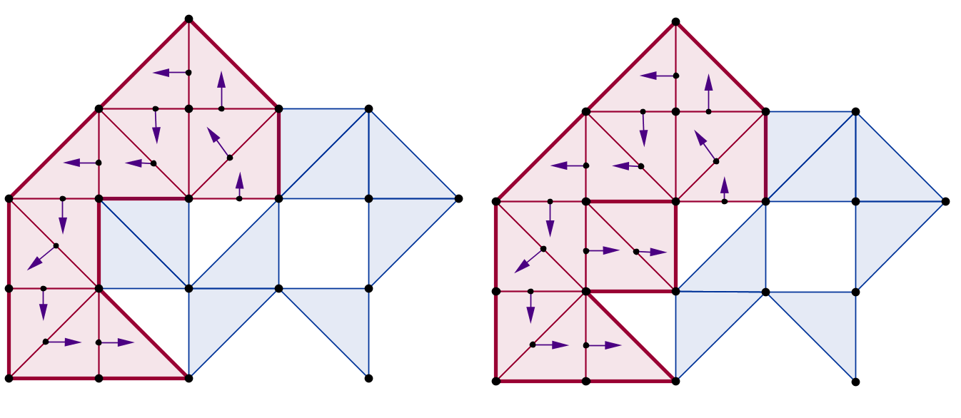
Figure 8: Frame Expansion: Example 2. Part I

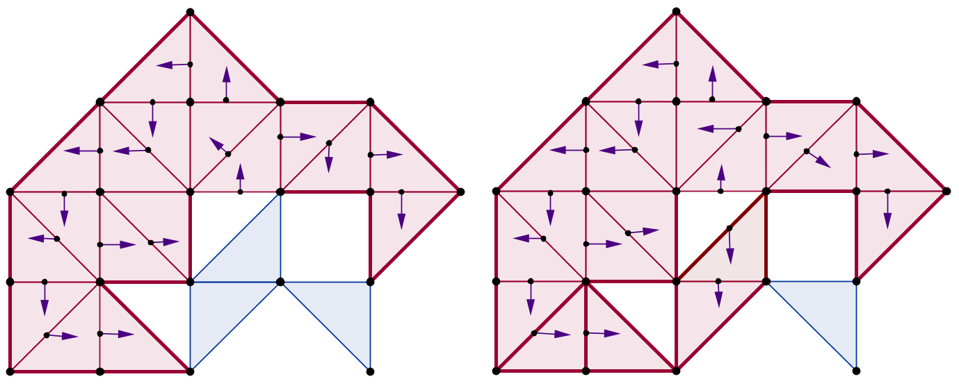
Figure 9: Frame Expansion: Example 2: Part II

Case 2: Suppose $\mathcal{M}$ has some 1-dim. boundary faces. In this case, $\mathcal{G}_{s}(\mathcal{M})$ has the structure of a possibly disconnected semigraph. If the manifold has a coboundary face, say $B_{1}$ then for the first connected component of $\mathcal{G}_{s}(\mathcal{M})$ in lines 18-19 of Procedure frameflow() in 2, we add the boundary-coboundary pair to vector field $\mathscr{V}$. Following that, the cells that are in the same connected component are added to the vector field in a manner similar to Case 1. If there exists another connected component, then surely such a connected component must have at least one coboundary face. In lines 31 and 30 of Procedure frameflow() in 2, we check if such a coboundary face exists. If it does exist then in the loop 15-31, we process the every connected component in the same way as we process the very first one. Given the fact that all connected components of semigraph $\mathcal{G}_{s}(\mathcal{M})$ are processed, every 2-cell $\varpi_{\textsf{new}}$ in each of these components is part of vector field $\mathscr{V}$. Suppose $\varpi_{\textsf{new}}$ is paired with some 1-cells $\vartheta_{\textsf{new}}$ each time then, each time we delete $\vartheta_{\textsf{new}}$ from the the frame and add $\mathcal{B}(\mu\setminus\vartheta_{\textsf{new}})$ to the frame. When new gradient pairs are processed, we may delete 1-cells from out frame, but 0-cells are never deleted. Since every vertex is incident on at least one of the 2-cells in one of the connected components, we establish the fact that all vertices eventually become part of the expansion frame. See Figure 8, Figure 9 and Figure 10 for such an example. ∎

Every connected component of $\mathcal{G}_{s}(\mathcal{M})$ has a 2-cell which shares a 0-cell with a 2-cell from another connected component. If we imagine every connected component of $\mathcal{G}_{s}(\mathcal{M})$ as a vertex and every shared 0-cell as a hyperedge then we get a connected hypergraph that we write as $\mathcal{H}_{c}(\mathcal{M})$. We know that $\mathcal{H}_{c}(\mathcal{M})$ is connected because if this were not the case then clearly $\mathcal{M}$ itself will have more than one connected components. We call $\mathcal{H}_{c}(\mathcal{M})$ the component hypergraph of $\mathcal{M}$.

Consider a gradient vector field $\mathcal{V}$ assigned to a manifold$\mathcal{M}$. First consider the case when $\mathcal{M}$ is a manifold without boundary. Consider a critical cell $\alpha^{2}$. Note that before we do any expansions, $\mathcal{B}(\alpha)$ is our original $\underline{\widehat{\alpha}}$. Let $\sigma\succ\tau\prec\alpha$. If $\langle\tau,\sigma\rangle\in\mathcal{V}$ then we can consider it as an expansion along $\tau$ to the cell $\sigma$. Now, as per the definition of frame expansion, we add the set $\{\mathcal{B}(\sigma)\setminus\{\tau\}\}$ to $\underline{\widehat{\alpha}}$ and we delete $\{\tau\}$ from $\underline{\widehat{\alpha}}$. Therefore,

$$\underline{\widehat{\alpha}}=\underline{\widehat{\alpha}}-\{\tau\}+\{\mathcal{B}(\sigma)\setminus\{\tau\}\}$$

But, this is same as saying, $\underline{\widehat{\alpha}}=\{\mathcal{B}(\alpha)\setminus\{\tau\}\}+\{\mathcal{B}(\sigma)\setminus\{\tau\}\}$. Clearly, the sets $\{\mathcal{B}(\alpha)\setminus\{\tau\}\}$ and $\{\mathcal{B}(\sigma)\setminus\{\tau\}\}$ are themselves connected and both these sets have a common boundary namely $\mathcal{B}(\tau)$ (the boundary of $\tau$). Therefore, expansion along $\tau$ preserves the connectivity of $\underline{\widehat{\alpha}}$. Now, given our intermediate stage $\underline{\widehat{\alpha}}$, if any of the 1 dim. cells say $\vartheta_{i}^{1}\in\underline{\widehat{\alpha}}$ forms a gradient pair with a $2$ dim. cell $\varpi_{i}^{2}$ then by expansion we have,

$$\underline{\widehat{\alpha}}=\underline{\widehat{\alpha}}-\{\vartheta_{i}\}+\{\mathcal{B}(\varpi_{i})\setminus\{\vartheta_{i}\}\}$$

Each time we observe that the boundary of $\underline{\widehat{\alpha}}$ and the boundary of $\{\mathcal{B}(\varpi_{i})\setminus\{\vartheta_{i}\}\}$ is, in fact, the same as the boundary of $\vartheta_{i}$ namely $\mathcal{B}(\vartheta_{i})$. Therefore, upon expanding the frame $\underline{\widehat{\alpha}}$ along $\vartheta_{i}$, connectivity of $\underline{\widehat{\alpha}}$ is preserved and $\underline{\widehat{\alpha}}$ continues to be a 1-manifold without boundary. Note that owing to the manifold nature of $\mathcal{M}$, $\{\mathcal{B}(\varpi_{i})\setminus\{\vartheta_{i}\}\}$ never contains a $(1)$-dimensional face, say $\vartheta_{j}$ (where $j<i$), along which $\underline{\widehat{\alpha}}$ was previously expanded. Therefore, because $\mathcal{M}$ is a manifold, the two encounters of $\vartheta_{j}^{1}$ can happen in two different ways, namely:
Case 1: While constructing $\underline{\widehat{\alpha}}$ through expansions, any face $\vartheta_{j}^{1}$ can be encountered at most twice - once when it is included in $\underline{\widehat{\alpha}}$ as part of some $\{\mathcal{B}(\varpi_{k})\}$ ($k<j$) and a second time if and when we expand along $\vartheta_{j}^{1}$. Even as we expand along $\vartheta_{j}^{1}$, the two vertices of $\vartheta_{j}^{1}$ stay connected.
Case 2: The other possibility of two encounters for the face $\vartheta_{j}^{1}$ is when it is included in $\underline{\widehat{\alpha}}$ as part of some $\{\mathcal{B}(\varpi_{k})\}$ ($k<j$) and some $\{\mathcal{B}(\varpi_{h})\}$ ($h<j$). In this case, we never expand along $\vartheta_{j}^{1}$.
If $\mathcal{M}$ has boundary then our start cell is a coboundary face and upon first expansion, the frame is a manifold with a boundary. Applying the reasoning above, for a given connected component of $\mathcal{G}_{s}(\mathcal{M})$, the frame of expansion restricted to a single connected component of $\mathcal{G}_{s}(\mathcal{M})$ is a connected 1-manifold without boundary. To arrive at the more general conclusion that the frames of expansion of all connected components of $\mathcal{G}_{s}(\mathcal{M})$, pieced together form a single connected 1-complex connecting all 0-cells of manifold $\mathcal{M}$, we have the lemma below:

Lemma 26.

Given any sequence of elementary expansions, the frame of a critical cell $\alpha^{2}$ of a manifold $\mathcal{M}$ is always a connected set. Following the final expansion, the frame consists of a set of edges that connects all vertices of the complex.

Proof.

Consider without loss of generality, that $\mathcal{M}$ is a manifold without boundary. Then $\mathcal{G}_{s}(\mathcal{M})$ has a single connected component. Every vertex within the frame that was previously connected, stays connected by 24. Since, for a manifold without boundary, the frame always has a single connnected component at every stage of expansion, and since by 25, all vertices become part of the frame, we arrive at the conclusion that all vertices of the frame form a single connected component at the conclusion of all expansions.
The other case, when $\mathcal{G}_{s}(\mathcal{M})$ has several connected components, we first observe that the frames of each of the connected component stays connected by the same logic as in case of expansions of manifolds without boundary. Also, we observe that in such cases, every connected component will have a 2-cell which is connected to another connected component via a common 0-cell. In fact, if there exist vertices $v_{a}$ and $v_{b}$ in two different connected components $C_{a}$ and $C_{b}$. $C_{a}$ and $C_{b}$ may be interpreted as vertices in the hypergraph then we can first determine a path between $C_{a}$ and $C_{b}$ within the component hypergraph $\mathcal{H}_{c}(\mathcal{M})$. Now, every vertex $C_{i}$ in the path is a connected component and every hyperedge is a shared 0-cell $v_{i}$. If the path is written as $C_{0},v_{1},C_{1},\dots,v_{i},C_{i},\dots v_{n},C_{n}$ where $C_{0}=C_{a}$ and $C_{n}=C_{b}$. Then for every $C_{i}$ $1<i<n$, we can determine an internal path (part of the expansion frame) in graph $\mathcal{G}_{s}(\mathcal{M})$ between $v_{i}$ and $v_{i+1}$. Finally, in graph $\mathcal{G}_{s}(\mathcal{M})$, we can find a path between $v_{a}$ and $v_{1}$ within component $C_{0}$ and a path between $v_{n}$ and $v_{b}$ within component $C_{n}$ as parts of expansion frames within those components. If we piece together each of the paths from expansion frames of various components of $\mathcal{G}_{s}(\mathcal{M})$ along the path in the hypergraph $\mathcal{H}_{c}(\mathcal{M})$, we get a path connecting any two vertices $v_{a}$ and $v_{b}$ such that every edge in the path is part of the expansion frame. From this we conclude that all vertices in the complex are connected to each other through edges that lie entirely in the expansion frame. In other words, the expansion frame is a single connected component that connects all vertices of the complex. ∎

Lemma 27.

Applying the frame based algorithm on a 2-manifold gives us:

$$c_{2}=\beta_{2}$$

Proof.

Case1: $\beta_{2}=1$ Suppose the 2-manifold does not have a boundary. Then clearly $\beta_{2}=1$. Now we will prove that in this case, $c_{2}$ also equals $1$. Recall that $\mathcal{G}_{s}(\mathcal{M})$ takes the structure of a simple connected graph and the procedure frameflow is equivalent to a breadth first traversal that begins with a start cell $\varpi$, where $\varpi$ is not included in any of the gradient pairs. However, subsequently every neighboring 2-cell is paired with a 1-cell and added to a queue. The neighbors of the dequeued cell are then scanned and if unpaired, they are paired with the connecting 1-cell as before. This process is continued till all 2-cells are exhausted (which happens at the conclusion of the breadth first traversal). Hence all 2-cells except the start 2-cell $varpi$ form a gradient pair with some 1-cell, giving us $c_{2}=1$.
Case2: $\beta_{2}=0$ Now, consider the case when the 2-manifold has a boundary. So, we have $\beta_{2}=0$ and we will prove that $c_{2}$ also equals $0$. Note that, in this case, $\mathcal{G}_{s}(\mathcal{M})$ has one or more connected components s.t. each of the connected components has at least one coboundary face. For every component a coboundary face is selected as a start cell and paired with a boundary face to give a gradient pair. Subsequently, as before neighboring 2-cells are paired with connecting 1-cells if they haven’t been paired before. Newly paired 2-cells are queued and this process continues till all 2-cells of the connected component are exhausted. In other words, every 2-cell of every connected component is part of a gradient pair giving us $c_{2}=0$. Hence proved. ∎

Let $\mathcal{B}^{1}$ be the coboundary of residual complex $\mathcal{M}$. $\mathcal{B}^{1}[i]$ is part of the coboundary $\mathcal{B}^{1}$ that intersects with ear $\mathcal{E}_{i}$. i.e. $\mathcal{B}^{1}[i]=\mathcal{B}^{1}\cap\mathcal{E}_{i}$.

Lemma 28.

If the complex is made up of a single connected component, then the frame based algorithm gives us $c_{0}=1$.

Proof.

From 26, we know that the frame of expansion consists of a single connected component that connects all 0-cells in the manifold. This frame is divided into $\mathscr{N}$ several ears say $\mathcal{E}_{i}$. Every ear is a 1-dimensional manifold. Suppose that we have an open ear then we have 1-dimensional coboundary face in such a ear which we pair with a 0-dimensional boundary face. Subsequently, we follow a path which matches the incident unpaired 0-cell to a neighboring 1-cell and we keep doing this until all 1-cells of the ear are exhausted. Now suppose that we have a closed ear. Then we remove one of the 1-cells from the ear (i.e. make it critical). This disconnects the ear into two connected components. We treat these two components of the ears as separate and proceed as in case of open ears. We now make an inductive argument to prove that the first ear leaves a critical 0-cell. Subsequent addition of ears do not add any criticalities. To see this consider the base case in which we design the flow for the first ear. Here, the flow stops when all 1-cells are exhausted. In this case, for the final 1-cell $\mu$, there is one 0-cell which gets paired with $\mu$ and another incident 0-cells which remains unpaired. It is this 0-cell that becomes the sole critical 0-cell. For induction consider the inductive hypothesis that k-ears have been attached and the number of critical cells remains 1. Now suppose that the (k+1)th ear is attached. If the (k+1)th ear is open then the flow stops with a 1-cell on which one of the incident 0-cells $v_{i}$ belongs to a ear $\mathcal{E}_{i}$ where $i<(k+1)$. Either $v_{i}$ is the sole critical 0-cell or it is paired to another 1-cell belonging to $\mathcal{E}_{i}$ (by inductive hypothesis). Now, suppose that the (k+1)th ear is closed. Then having detached a 1-cell (which is made critical), we have two disconnected components. For each of the connected components, the flow emanating from subsequent pairing of 0-cells to 1-cells stops when a 1-cell is incident on a 0-cell $v_{j}$ belonging to a ear $\mathcal{E}_{j}$ where $j<(k+1)$. Once again by inductive hypothesis either $v_{j}$ is the sole critical 0-cell or it is paired to another 1-cell belonging to $\mathcal{E}_{j}$. From this we conclude that $c_{0}=1$ on attachment of all ears. ∎

Theorem 29.

For the frame-based vector field design algorithm, each Morse number equals the Betti number. i.e.

$$c_{i}=\beta_{i}$$

Proof.

From 27 and 28, we have $c_{2}=\beta_{2}$ and $c_{0}=\beta_{0}$ respectively. Now, using Equation 2 in Theorem 8, we have $c_{1}=\beta_{1}$. Thus we have $c_{i}=\beta_{i}$ for all $i$. ∎

3.4 Discussion on Complexity

Finding coboundary of $\mathcal{M}^{2}$ can be found in linear time by going through all 2-cells in $\mathcal{M}^{2}$. Finding coboundary of ears of $\mathscr{M}$ can be found in constant time by mainting a proper data structure. The ear decomposition of residual complex $\mathscr{M}$ (which has the structure of a graph) itself takes linear time.

Adding a gradient pair to a vector field takes constant time. The queueing, dequeueing and deletion operations also can be done in constant time by maintaining appropriate data structures.

The only nontrivial procedure in the algorithm is frameflow(). Now the frameflow() procedure can be construed as breadth first traversal on a semi-graph. We apply this procedure once on $\mathcal{M}^{2}$ and once on each of the ears of $\mathscr{M}$. When traversals from all ears are counted, we observe that every edge of $\mathscr{M}$ is encountered only once and every vertex $v_{i}$ is encountered $\mathcal{D}(v_{i})$ number of times where $\mathcal{D}(\cdot)$ indicates degree of a vertex. So, if we sum over all vertices and edges, the total complexity of frameflow() when applied over $\mathscr{M}$ is linear in the number of edges of $\mathscr{M}$. Hence, we see that the design of optimal discrete gradient vector field using expansion frames takes linear time.

4 Pseudo-optimality of Random Morse functions

In this section, we establish the surprising potency of critical cell cancellations in case of 2-manifolds by using frames.

Definition 30 (Pseudo-optimal Vector Field).

We define a DGVF to be pseudo-optimal if the optimal DGVF can be obtained from it merely via critical cell cancellations.

Definition 31 (Stable, Unstable Manifolds).

The stable manifold of a critical cell $\alpha^{q}$ are all the non-critical cells of dimension $q$ and $q+1$ with gradient paths ending at $\alpha^{q}$. The unstable manifold of a critical cell $\alpha^{q}$ are all the non-critical cells of dimension $q$ and $q-1$ with gradient paths starting at $\alpha^{q}$ and ending at that particular non-critical cell.

1:procedure kingRev($\mathfrak{K}^{q},\mathcal{M},\mathcal{C},\mathscr{V},q$)

2:   repeat

3:         Suppose critical cells $\sigma^{q}$ and $\mathfrak{K}^{q}$ have gradient paths to/from saddle $\gamma^{1}$.

4:         Subroutine sharedSaddle() finds such a pair $\{\gamma,\sigma\}$ for given $\mathfrak{K}$.

5:         If $\gamma\neq\textsf{NIL}$, then cancel critical pair $(\gamma,\sigma)$

6:   until $(\gamma\neq\textsf{NIL})$

7:   If $q=2$ AND $\mathfrak{K}^{q}$ has a unique path to $\phi^{1}$, then cancel critical pair $(\phi,\mathfrak{K})$

8:end procedure

9:

10:procedure fixBdry($d,p,\mathcal{M},\mathcal{C}^{p},\mathcal{B}^{d}$)

11:   for $1\leq i\leq|\mathcal{B}^{d}|$ do

12:         Let $B_{i}\colonequals\mathcal{B}^{d}[i]$ and let $b_{ij}$ be a boundary face of $B_{i}$.

13:         if $\langle b_{ij},B_{i}\rangle\notin\mathcal{V}\textsf{ AND }b_{ij}\textsf{ is critical}$ then

14:               Let $\langle\theta_{i},B_{i}\rangle$ be a gradient pair

15:               if $\theta_{i}\neq\textsf{NIL}$ and $\theta_{i}$ is not a boundary face of $B_{i}$ then

16:                     Find a gradient path from some critical cell $\alpha^{d}$ to $\theta_{i}$ and reverse it.

17:               end if

18:               Add gradient pair $\langle b_{ij},B_{i}\rangle$ to vector field $\mathscr{V}$

19:         end if

20:   end for

21:end procedure

22:

23:procedure findKing($d,p,\mathcal{M},\mathcal{C}^{p},b^{q},i$)

24:   if$\left(p=2\textsf{ AND }\mathcal{C}^{p}\neq\textsf{NIL}\right)\textsf{ OR }(p=1\textsf{ AND }i=1)$ then  $\textbf{remFrom}(\mathcal{C}^{p},\mathfrak{K})$;

25:   else if $p=1$ then $\mathfrak{K}\colonequals b^{q}[1]$; $\textbf{remFrom}(b^{q},\mathfrak{K})$;

26:   else $\mathfrak{K}\colonequals\textsf{NIL}$;

27:   end if

28:   $\mathfrak{K}\colonequals\textbf{selectRandomly}(\mathcal{C}^{p})$;   return $\mathfrak{K}$;

29:end procedure

30:

31:procedure processComplex($\mathcal{M},i,d,p$)

32:   $\mathcal{C}[1:d]\leftarrow\textbf{identifyCritical}(\mathcal{M},\mathscr{V})$

33:   $\textbf{findBdry}()$ finds $\mathcal{B}^{d}$ & $b^{d-1}$ the cobdry. and bdry. of $\mathcal{M}$ resp.

34:   $\textbf{fixBdry}(d,p,\mathcal{M},\mathcal{C}^{d},\mathcal{B}^{d})$

35:   while ($\mathfrak{K}=\textbf{findKing}(d,p,\mathcal{M},\mathcal{C}^{p},b^{d-1},i)\neq\textsf{NIL}$ do

36:         $\textbf{kingRev}(\mathfrak{K},\mathcal{M},\mathcal{C},\mathscr{V},p)$

37:   end while

38:end procedure

39:

40:procedure kingFlow($\mathfrak{M},d,\mathscr{V}$)

41:   Divide $\mathfrak{M}$ into manifolds $\mathcal{M}_{1},\mathcal{M}_{2},\dots,\mathcal{M}_{K}$ s.t. $\mathcal{M}_{i}\cap\mathcal{M}_{j}$ is 0-dimensional.

42:   for $1\leq i\leq K$ do  $\textbf{processComplex}(\mathcal{M}_{i},i,2,2)$ end for

43:   $\mathcal{E}[1:\textsf{numEars}]\colonequals\textbf{earDecompose}(\mathscr{M}$)

44:   for $1\leq i\leq\textsf{numEars}$ do  $\textbf{processComplex}(\mathcal{E}[i],i,1,0)$  end for

45:end procedure

Algorithm 3 Optimal DGVF Redesign Using Critical Cell Cancellations

Given a connected pseudomanifold complex $\mathfrak{M}$, divide $\mathfrak{M}$ into several connected components $\mathcal{M}_{1},\mathcal{M}_{2},\dots,\mathcal{M}_{K}$ s.t. $\mathcal{M}_{i}\cap\mathcal{M}_{j}$ is 0-dimensional. i.e. any of the two manifolds (with boundary) $\mathcal{M}_{i},\mathcal{M}_{j}$ may intersect only along points (but not along edges). If $\mathfrak{M}$ is a manifold without boundary then $\mathfrak{M}$ will have only one connected component. $\mathcal{M}_{i}$ are essentially the connected components of the semigraph $\mathcal{G}_{s}(\mathcal{M})$ defined in 24.

Lemma 32.

If $\mathfrak{M}$ is a manifold without boundary then after invoking the procedure kingRev(), we obtain a connected expansion frame. Moreover, $c_{2}=\beta_{2}=1$.

Proof.

Suppose a vector field $\mathscr{V}$ on manifold $\mathfrak{M}$ (without boundary) has a single critical cell. Then from 26, we get a single connected expansion frame connecting all vertices of $\mathfrak{M}$. Instead, if $\mathfrak{M}$ is a manifold without boundary and if we have more than one critical 1-cells, then consider the unstable manifold of some chosen critical cell $\mathfrak{K}$. Since the unstable manifold of $\mathfrak{K}$ doesnot include the entire manifold $\mathfrak{M}$, the stable manifold has a 1-dimensional manifold as its boundary. From [12], we know that, if $\mathcal{M}$ is an n-dimensional manifold with boundary, then the boundary of $\mathcal{M}$ is an (n-1)-dimensional manifold (without boundary) when endowed with the subspace topology. Therefore, the boundary of the unstable manifold is a 1-dimensional manifold without boundary (i.e. it consists of one or more disjoint circles). Clearly the 1-cells belonging to this boundary are not part of the 2-flow of $\mathscr{V}$, else they wouldn’t be part of the boundary of the unstable manifold of $\mathfrak{K}$. So, the 1-cells belonging to this boundary are either part of the 1-flow of $\mathscr{V}$ or they are critical. Consider one of the disjoint circles that forms part of the boundary of the unstable manifold. If all the cells on this circle are part of the 1-flow then it will form a cycle. Hence there exists at least one critical 1-cell on the boundary of the unstable manifold. Let $\gamma$ be a critical that lies on the boundary of the unstable manifold of $\mathfrak{K}$. Clearly, there exists only one gradient path from $\mathfrak{K}$ to $\gamma$. $\gamma$ is also incident on a 2-cell say $\sigma_{1}$ that does not lie in the unstable manifold of $\mathfrak{K}$. Suppose $\sigma_{1}$ is itself a critical 2-cell, then $\gamma$ lies on the boundary of unstable manifolds of the two critical 2-cells $\mathfrak{K}$ and $\sigma_{1}$. Otherwise suppose that $\sigma_{1}$ is matched. Because the simplicial complex $\mathfrak{M}$ is a manifold, it is possible to trace any inverted gradient path on $\mathfrak{M}$ (such a unique inverse gradient path exists). Therefore, we trace the inverted gradient path $\gamma,\sigma_{1},\dots$ until we reach a critical 2-cell (say $\sigma_{k}$) from which this path emanates. In any case, we can find a critical 1-cell $\gamma$ which is shared by critical cells $\mathfrak{K}$ and some other critical 2-cell say $\sigma$. In this case, because gradient path from $\sigma$ to $\gamma$ is unique we can invert this gradient path as shown in Line 6 of Procedure kingRev() of 3. Once this cancellation is done, the unstable manifold of $\sigma$ becomes part of the new unstable manifold of $\mathfrak{K}$. Once again we search a critical 1-cell $\gamma_{2}$ on the boundary of the unstable manifold s.t. which also lies on the boundary of unstable manifold of some other critical 2-cell (distinct from $\mathfrak{K}$). If such a pair of critical cells is found then we cancel it and this procedure is repeated until all critical 2-cells belong to the unstable manifold of $\mathfrak{K}$ (or alternatively all critical 1-cells have two gradient paths from $\mathfrak{K}$.) Basically this means that $\mathfrak{M}$ is a manifold without boundary that has a unique critical 2-cell. i.e. $c_{2}=1$. Since, $\mathfrak{M}$ is a 2-manifold without boundary, $\beta_{2}=1$. Finally, from Case 1 of 27, we arrive at the conclusion that the expansion frame is a connected 1-manifold that includes all 0-cells of $\mathfrak{M}$. ∎

If $\mathfrak{M}$ is a manifold without boundary then $\mathcal{G}_{s}(\mathcal{M})$ has a single connected component and the for loop described in Lines 42-42 of Procedure kingFlow() in 3 gets executed only once. Also the while loop described in Lines 35-37 of Procedure processComplex() in 3 gets executed only once for manifolds without boundary. This is because for any critical 2-cell $\mathfrak{K}$, you always find another critical 2-cell $\sigma$ s.t. both $\mathfrak{K}$ and $\sigma$ have a gradient path to a common 1-cell $\gamma$ unless the unstable manifold of $\mathfrak{K}$ covers the entire manifold $\mathfrak{M}$.
The situation is however much different for a manifold with boundary. For such a manifold the for loop and the while loop may run several iterations.

Lemma 33.

If $\mathfrak{M}$ is a manifold with boundary then after invoking the procedure kingRev(), we obtain a connected expansion frame. Moreover, $c_{2}=\beta_{2}=0$.

Proof.

We will examine the effect of the algorithm on one of the connected components $\mathcal{M}_{i}$ of $\mathcal{G}_{s}(\mathcal{M})$. Consider the unstable manifold of a critical 2-cell $\mathfrak{K}$. From [12], we know that, if $\mathcal{M}$ is an n-dimensional manifold with boundary, then the boundary of $\mathcal{M}$ is an (n-1)-dimensional manifold (without boundary) when endowed with the subspace topology. Hence, the boundary of this unstable manifold will be a 1-manifold without boundary (i.e. a disjoint set of circles). The 1-cells on any one of these circle are involved only in 1-flows or they are critical. But all, cells of a circle can not be involved in 1-flow as this would lead to a cycle in the vector field. So, every circle must contain a 1-cell, say $\gamma$ that is critical. $\mathfrak{K}$ has only one gradient path to $\gamma$. There exists a second gradient path that ends at $\gamma$. This gradient path either emanates from another critical 2-cell say $\sigma$ or it emanates from a boundary face. Assume the case where a path to $\gamma$ emanates from $\sigma$. In this case, the pair $(\gamma,\sigma)$ is detected and cancelled in Lines 3-6 of Procedure kingRev() in 3. In fact, every such pair $(\gamma,\sigma)$ for a given $\mathfrak{K}$ is detected and cancelled in the loop Lines 3-6 of Procedure kingRev() in 3. So finally every critical 1-cell say $\phi$ in the boundary of the unstable manifold of $\mathfrak{K}$ will have a second path emanating from a boundary face. In this case, the pair of critical cells $(\phi,\mathfrak{K})$ is detected and cancelled as shown in Line 7 of Procedure kingRev() in 3. Suppose that $\mathcal{M}_{i}$ continues to have critical cells that are not cancelled, then a new critical king cell $\mathfrak{K}$ is selected and the same procedure as described above is repeated in a loop shown in Lines 35-37 of Procedure processComplex in 3. We exit from the loop provided there are no other critical 2-cells to process in the list $\mathcal{C}^{p}$. In case of manifolds with boundary every critical 2-cell processed as a king cell $\mathfrak{K}$ is itself cancelled along with cancelling all the neighboring critical 2-cells that share gradient paths to the same saddles as $\mathfrak{K}$. Having processed $\mathcal{M}_{i}$ in this manner, we are assured that eventually $\mathcal{M}_{i}$ has no critical 2-cells. In fact every 2-flow for $\mathcal{M}_{i}$ emanates strictly from boundary faces. Using an argument similar to that in Case 2 of 27, we know that the frame of expansion of a boundary face is a connected set. Consider the first such boundary face $b_{1}$, with a frame of expansion which is a connected 1-manifold. Every 1-cell belonging to the frame of expansion of $b_{1}$ has a second gradient path emanating from other boundary cells $\{b_{i}\}$. Since the $\mathcal{M}_{i}$ is a manifold with boundary, given any pair of boundary faces $b_{i},b_{j}$, we can find a type 2 connected 2-path between them. Consider all the 1-cells in some such type 2-connected path between $b_{i}$ and $b_{j}$. Every 1-cell either lies in the frame of expansion of two boundary faces or is involved in 2-flow with a regular 2-cell. This gives us a sequence of frames of expansion of boundary faces $b_{k_{1}},b_{k_{2}},\dots,b_{k_{L}}$ that are sequentially pairwise connected and s.t. $b_{k_{1}}=b_{i}$ and $b_{k_{L}}=b_{j}$. Since this procedure can be applied to any two boundary faces (with expansion frames), we conclude that the set of frames of expansion of all boundary faces is a connected set, which we refer to as the expansion frame of $\mathcal{M}_{i}$. To see that the frame of expansions of all $\mathcal{M}_{i}$ form a single connected set, we consider the component hypergraph $\mathcal{H}_{c}(\mathcal{M})$. We then use the same line of reasoning as used in 26, to conclude that the expansion frame of $\mathfrak{M}$ is connected. Also, following all critical cell cancellations since there are no more critical 2-cells for $\mathcal{M}_{i}$, we have $c_{2}=\beta_{2}=0$ for each $\mathcal{M}_{i}$. So, we have also have $c_{2}=\beta_{2}=0$ for $\mathfrak{M}$ ∎

The residual 1-complex $\mathscr{M}$ is essentially the expansion frame of $\mathfrak{M}$ following cancellation of critical cell pairs of dimensions $1,2$. Since there exists a preordained 1-flow (without cycles) on $\mathscr{M}$, clearly given the mechanism of discrete Morse theory, there must exist at least one critical 0-cell. (A sub-optimal 1-flow may have more than one critical 0-cells. But at least one is guaranteed.) The first ear is chose to be one that includes at least one of these critical 0-cells. Also the ear decomposition follows a special procedure. The number of ears are determined by the number of unstable manifolds of boundary 0-cells and critical 1-cells. The first ear is either an unstable manifold of a boundary 0-cell or a critical 1-cell that includes at least one critical 0-cell. The second ear is a 1-manifold that is incident on a 0-cell that belongs to the $1^{st}$ ear and includes all the 0-cells and 1-cells of an unstable manifold of a boundary 0-cell or a critical 1-cell that aren’t already included in the first ear. The $k^{th}$ ear is a 1-manifold that is incident on a 0-cell that belongs to one of the previous $(k-1)$ ears and includes all 0-cells and 1-cells of an unstable manifold of a boundary 0-cell or a critical 1-cell that aren’t already included as part of the previous $(k-1)$ ears. Every ear (apart from the first ear), has at least one 0-cell in its 0-dim. boundary whereas every ear may have at most two 0-cell in its 0-dim. boundary. The first boundary cell of the ear $b^{0}[1]$ is incident on one of the previous ears. The second boundary cell $b^{0}[2]$ may or may not be incident on any of the previous ears.

Lemma 34.

On applying a series of critical cell cancellations, the connected expansion frame has $c_{0}=\beta_{0}=0$

Proof.

We shall make an inductive argument. The idea is that the first ear will have a 0-cell that is critical. Subsequent ears attached to the first ear have no 0-dimensional critical cells. Note that all ears are 1-dimensional manifolds (topological circles or topological line segments)
Base Case: Suppose that we start with the first ear. Suppose that the first ear is a closed loop (i.e. a topological circle). From section 4 our first ear has at least one critical 0-cell. Suppose we call it $\varrho^{0}$. In this case $\varrho$ becomes our king critical cell $\mathfrak{K}$. If there exist two gradient paths to $\varrho$ from a saddle, then clearly we do not have any criterion for cancellation. Instead if we have a single gradient path from the saddle $\gamma^{1}$ and suppose there exists another gradient path from the $\gamma$ to some other minima $\varphi^{0}$ then from Lines 3-6 of Procedure kingRev() in 3, we cancel critical pair $(\varphi,\gamma)$ and as a result have a single critical 0-cell in the first ear. The last possibility the first ear consists of the unstable manifold of a critical 0-cell $\varsigma$ that $\varrho^{0}$
Induction step: By the inductive hypothesis, we have processed $(k-1)$ ears so far and for all the $(k-1)$ ears taken together, we have only one critical 0-cell (namely the one that was encountered in the very first ear.) Now, we need to establish that on attachment of the $k^{th}$ ear we do not introduce any new critical 0-cells. Note that for $k^{th}$ ear we start with $b^{0}[1]$ as the king cell $\mathfrak{K}$, where $b^{0}[1]$ is incident on one of the previous ears (i.e. it may either be our original critical cell $\varrho^{0}$, or it may be some regular 0-cell from one of the earlier $(k-1)$ ears. Like all other ears, the $k^{th}$ ear is an unstable manifold of a boundary 0-cell or a critical 1-cell. If it is the unstable manifold of a boundary 0-cell $\varsigma$ then we do not have anything to prove as the flow for this cell will simply start with $\varsigma$ and end at $b^{0}[1]$ without introducing any criticalities. If the $k^{th}$ ear is topologically a loop, then $b^{0}[1]$ has two gradient paths from some saddle $\gamma$ and hence the criterion for cancellation is not satisfied. Yet another case is when $b^{0}[1]$ and $b^{0}[2]$ are both incident on one of the earlier $k$ ears. In this case, $b^{0}[1]$ is either $\varrho$ or a regular 0-cell and $b^{0}[2]$ is certainly a regular cell. Also, there does not exist any other critical 0-cell in this ear because the $k^{th}$ ear, in this case, is an unstable manifold of a saddle. The only interesting case is when $k^{th}$ ear is topologically a line segment s.t. $b^{0}[2]$ is critical and the saddle $\gamma$ has one gradient paths each to $b^{0}[1]$ and $b^{0}[2]$. Since, for $k^{th}$ ear we start with $b^{0}[1]$ as king cell $\mathfrak{K}$, we end up cancelling $\gamma$ and $b^{0}[2]$, making the $k^{th}$ ear an unstable manifold of boundary cell $b^{0}[2]$. In each of the cases, we ensure that either the $k^{th}$ ear did not have any critical 0-cell to begin with or if there does exist a critical 0-cell, then it is cancelled. Hence proved. ∎

Theorem 35.

Every discrete gradient vector field on a 2-manifold is pseudo-optimal.

Proof.

Suppose that at the end of the first call to Procedure findKing() from Line 35 of Procedure processComplex() in 3, $\mathfrak{K}^{2}$ is not NIL. Then, we claim that the unstable manifold of $\mathfrak{K}^{2}$ does not have any critical 1-cells that are boundary faces. This is because, if $\mathfrak{K}^{2}$ did have any boundary critical 1-cells in its unstable manifold, it would have got cancelled in the loop shown in Lines 11-20 in Procedure fixBdry() in 3. In fact, more generally every critical 2-cell at the end of first call to Procedure findKing() will have no critical boundary 1-cells in their respective unstable manifolds. If $\mathfrak{M}$ is a manifold without boundary, then by 32, we have $c_{2}=\beta_{2}=1$ and we get a connected frame of expansion in form of residual complex $\mathscr{M}$. Instead, if $\mathfrak{M}$ is a manifold with boundary, then from 33 we obtain $c_{2}=\beta_{2}=0$ and a connected frame of expansion in form of residual complex $\mathscr{M}$. Given a connected frame of expansion $\mathscr{M}$, guarantees that we have $c_{0}=\beta_{0}=1$. Finally, using Weak Morse Inequlity we obtain $c_{1}=\beta_{1}$. Hence, we prove that for a 2-manifold, given an arbitrary vector field $\mathscr{V}_{1}$ merely by using critical cell cancellations, we may obtain the optimal vector field $\mathscr{V}_{2}$. In other words, every gradient vector field on a 2-manifold is pseudo-optimal. ∎

5 The Topological Explanation for simplicity of computation of $H(\mathcal{M}^{2},\mathbb{A})$

We compute homology using 1. Also we assume Weak Morse Optimality Condition as defined in 11 on the input.

As we can see from arguments in section 3, the topological explanation for simplicity of computation of homology groups for 2-manifolds is:

1. On 2-manifolds optimal Morse functions are perfect. In fact, 2-manifolds admit readily computable perfect Morse functions.

2. A 2-manifold has optimal $c_{2}=0$ or $c_{2}=1$, which can be figured out in linear time by examining whether or not it has a boundary.

3. We define and apply frames of expansion an elementary homotopy theory construct to design our algorithm.

4. It can be seen that irrespective of what traversal method we use to traverse the graph like connectivity structure of 1-cells and 2-cells of a 2-manifold, the frame of expansion remains connected. Furthermore, this connectivity guarantees that optimal $c_{0}=1$.

5. Finally weak Morse Inequality guarantees that our $c_{1}$ is optimal. i.e. $c_{1}=\beta_{1}$.

6. Moreover, our dynamic programming based boundary operator computation algorithm is pseudo-linear time (which becomes strictly linear assuming WMOC).

7. Finally, assuming WMOC, the application of Smith Normal Form (a supercubical time algorithm) on input of constant size is inexpensive.

8. The pseudo-optimality of arbitrary discrete Morse functions as outlined in section 4 further strengthens our argument about simplicity of computing optimal discrete Morse functions.

6 Concluding Remarks

In this work, we provide a nearly linear time algorithm for computing homology (with arbitrary coefficients) on 2-manifolds - the first such algorithm. This is particularly useful to compute homology of 2-manifolds that may have torsion elements. The design involves the introduction and usage of an elementary simple homotopy construct that we call expansion frames. Having designed the optimal Morse function in linear time, we use a dynamic programming based pseudo-linear time boundary operator algorithm for computing the Morse boundary operator. Assuming the sum of Betti numbers is a small constant compared to the size of the complex, the Smith Normal Form is applied to a very smal input, giving us near-linearity. Finally, using the notion of expansion frames, we prove an unexpected result in discrete Morse theory: Start with an arbitrary DGVF on a 2-manifold and one may obtain an optimal DGVF merely by application of critical cell cancellations.

Appendix

7 Elementary Algebraic Topology

[15]

Figure 2: 2-manifolds

Definition 36 (Simplicial Complex).

A simplicial complex $\mathcal{K}$ is a set of vertices and a collection $\mathcal{L}$ of subsets of vertices called faces. All faces satisfy the following property: The subset of a face is also a face. (i.e. $\mathcal{B}\in\mathcal{L},\mathcal{A}\in\mathcal{B}\Longrightarrow\mathcal{A}\in\mathcal{L}$). Maximal faces w.r.t. inclusion are known as facets. The dimension of a face $\mathcal{B}$ is defined to be $|\mathcal{B}|-1$. The dimension of the simplicial complex itself is the maximum over the dimension of its faces.

Definition 37 (Open Cell).

An n-dimensional open cell is a topological space that is homeomorphic to an open ball.

Definition 38 (Cell Complex).

A hausdorff topological space $X$ is called a finite cell complex if

1. $X$ is a disjoint union of open cells $\{D_{i}^{n}\}$ where $D_{i}^{n}$ is an open $n$-cell. ($i\in I$ where $I$ is the indexing set.)

2. For each open cell $D_{i}^{n}$ there is a map $\phi_{i}^{n}:B^{n}\to X$ such that $\phi_{i}^{n}$ restricted to the interior of the closed ball $B^{n}$ defines a homeomorphism to $D_{i}^{n}$ and such that $\phi_{i}^{n}(S^{n-1})$ is contained in the $(n-1)$-skeleton of $X$. (The $k$-skeleton of $X$ is the union of all open cells $D_{i}$ of dimension $r\leq k$).

3. Finally, a set $\alpha$ is closed in $X$ if and only if $\alpha\cap\overline{D}_{j}$ is closed in $\overline{D_{j}}^{n}$ for each cell $D_{j}^{n}$. Note that $\overline{D_{j}}^{n}=\phi_{i}^{n}(B^{n})$.

A cell complex is said to be regular if each $\phi_{i}^{n}$ is a homeomorphism and if it sends $S^{n-1}$ to a union of cells in the $(n-1)$-skeleton of $X$.

In lay man terms, to construct a cell complex you start with points $\mathcal{D}_{i}^{0}$, then glue on lines $\mathcal{D}_{i}^{1}$ to $\mathcal{D}_{i}^{0}$, then glue discs $\mathcal{D}_{i}^{2}$ to $\mathcal{D}_{i}^{1}$ and $\mathcal{D}_{i}^{0}$ and so on. Therefore a cell complex is a topological space constructed from a union of objects called cells, which are balls of some dimension, glued together on boundaries. Cell complexes are the most convenient object to do Algebraic Topology. But to simplify the discussion, we will instead provide a basic presentation of simplicial homology.

Notation 39.

Boundary & Coboundary of a simplex $\sigma$: We define the boundary $bd(\sigma)$ and respectively coboundary $\eth\>\sigma$ of a simplex as
$\eth\>\sigma\,=\>\{\tau\,|\,\tau\prec\sigma\}$ $\delta\>\sigma=\{\rho\,|\,\sigma\prec\rho\}$

Homology groups are the most important and general topological invariants of simplicial and cubical complexes, that are also computationally feasible. At the heart of it, Algebraic Topology is essentially the use of Linear Algebra to compute combinatorial topological invariants of a give space. Given a simplicial complex $W$, can define simplicial $q$-chains, which are formal sums of $q$-simplices $\sum_{s\in S}a_{i}s_{i}$ where the $a_{i}$ are integer coefficients. The abelian group of sums of $k$-simplices under addition is called the Chain Group and denoted by $C_{q}(W,\,\mathbb{Z})$. The $n$-simplex $\triangle=\{v_{0},v_{1},\cdots,v_{n}\}$with standard orientation is denoted $+\left[v_{0},v_{1},\cdots,v_{n}\right]$. Consider the permutation group of $n$-letters on the vertices of $\triangle$. The set of permutations fall into 2 equivalence classes: even permutations and odd permutations. The set of even permutations induce the positive orientation $+\left[v_{0},v_{1},\cdots,v_{n}\right]$ whereas the set of odd permutations induce the negative orientation $-\left[v_{0},v_{1},\cdots,v_{n}\right]$.

For each integer $q$, $C_{q}(W)$ is the free abelian group generated by the set of oriented $q$-simplices of $W$. Let $W_{q}$ be the total number of $q-$dimensional simplices for simplicial complex $W$. Then, one can show that $C_{q}\cong\mathbb{Z}^{W_{q}}$.

The boundary map $\partial_{q}$ is defined to be the linear transformations $\partial_{q}\,:\,C_{q}\rightarrow C_{q-1}$.

Examples of such operations are given in Fig.E3 and Fig.E4.

Figure 3: Dim 1 Boundary Operator

Figure 4: Dim II Boundary Operator

Figure 5: $\partial\partial=0$gives us a chain complex.

This map gives rise to a chain complex: a sequence of vector spaces and linear transformations:

$$0\stackrel{{\scriptstyle}}{{\rightarrow}}C_{n}\stackrel{{\scriptstyle\partial_{n}}}{{\rightarrow}}C_{n-1}\stackrel{{\scriptstyle\partial_{n-1}}}{{\longrightarrow}}...\stackrel{{\scriptstyle\partial_{q+2}}}{{\longrightarrow}}C_{q+1}(W)\stackrel{{\scriptstyle\partial_{q+1}}}{{\longrightarrow}}C_{q}(W)\stackrel{{\scriptstyle\partial_{q}}}{{\longrightarrow}}...\stackrel{{\scriptstyle\partial_{2}}}{{\rightarrow}}C_{1}(W)\stackrel{{\scriptstyle\partial_{1}}}{{\rightarrow}}C_{0}(W)\rightarrow 0.$$

It can easily be proved that that for any integer $q$,

$$\partial_{q}\circ\partial_{q+1}=0.$$

In general, a chain complex $C_{\star}=\left\{C_{q},d\right\}$ is precisely this : a sequence of abelian groups $\left(C_{q}\right)$ connected by an operator $d_{q}:C_{q}\to C_{q-1}$ that satisfies $d\circ d=0$.

If one defines

$$Z_{q}=\ker\partial_{q}\text{ and }B_{q}=\mathrm{im}\,\partial_{q+1},$$

then it follows that $B_{q}\subset Z_{q}$. Elements of $Z_{q}=\mathrm{ker}\partial_{q}$ are called cycles, and elements of $B_{q}=\mathrm{im}\partial_{q+1}$ are called boundaries. Likewise, $Z_{q}=\mathrm{ker}\partial_{q}$ is called the $q-$th Cycle Group and $B_{q}=\mathrm{im}\partial_{q+1}$ is called the $q-$th Boundary Group. Then the homology group $H_{q}$ measures the equivalence class of cycles by quotient-ing out the boundaries i.e. this construction measures how far the sequence is from being exact.

The $q$-dimensional homology of $W$, denoted $H_{q}(W)$ is the quotient vector space,

$$H_{q}(W)=\frac{Z_{q}(W)}{B_{q}(W)}\cdotp$$

and the $q$-th Betti number of $W$ is its dimension:

$$\beta_{q}=\dim H_{q}=\dim Z_{q}-\dim B_{q}$$

8 Morse Homology

Let $F$ be a Discrete Morse function defined on simplicial complex $W$. Let $C_{q}(W,\mathbb{\,Z})$ denote the space of $q$-simplicial chains, and $\mathcal{M}_{q}$ which is a subset of $C_{q}(W,\mathbb{\,Z})$ denote the span of the critical $q$-simplices. Let $\mathcal{M_{\star}}$ denote the space of Morse chains. Let $c_{q}$ denote the number of critical $q$-simplices. Then we have, $\mathcal{M}_{q}\cong\mathbb{Z}^{c_{q}}$.

Theorem 40 (Forman [6]).

There exist boundary maps $\widehat{\partial_{q}}\,:\,\mathcal{M}_{q}\rightarrow\mathcal{M}_{q-1}$, for each $q$, which satisfy

$$\widehat{\partial}_{q}\circ\widehat{\partial}_{q+1}=0.$$

and such that the resulting differential complex

$$0\stackrel{{\scriptstyle}}{{\longrightarrow}}\mathcal{M}_{n}\stackrel{{\scriptstyle\widehat{\partial}_{n}}}{{\longrightarrow}}\mathcal{M}_{n-1}\stackrel{{\scriptstyle\widehat{\partial}_{n-1}}}{{\longrightarrow}}\dots\stackrel{{\scriptstyle\widehat{\partial}_{q+2}}}{{\longrightarrow}}\mathcal{M}_{q+1}\stackrel{{\scriptstyle\widehat{\partial}_{q+1}}}{{\longrightarrow}}\mathcal{M}_{q}\stackrel{{\scriptstyle\widehat{\partial}_{q}}}{{\longrightarrow}}\dots\stackrel{{\scriptstyle\widehat{\partial}_{2}}}{{\longrightarrow}}\mathcal{M}_{1}\stackrel{{\scriptstyle\widehat{\partial}_{1}}}{{\longrightarrow}}\mathcal{M}_{0}\longrightarrow 0$$

calculates the homology of $W$. i.e. if we go with the natural definition,

$$H_{q}(\mathcal{M},\widehat{\partial})=\frac{\mathrm{ker}\widehat{\partial}_{q}}{\mathrm{im}\widehat{\partial}_{q+1}}$$

Then for each $q$, we have $H_{q}(\mathcal{M},\widehat{\partial})=H_{q}(W,\mathbb{Z})$.

Theorem 41 (Boundary Operator Computation. Forman [6]).

Consider an oriented simplicial complex. Then for any critical (p+1)-simplex $\beta$ set:

$\partial\beta=\sum\limits_{critical\>\alpha(p)}\>P_{\alpha\beta}\>\alpha$

$P_{\alpha\beta}=\sum\limits_{\gamma\in\Gamma(\beta,\alpha)}N(\gamma)$

where $\Gamma(\beta,\alpha)$ is the set of discrete gradient paths which go from a face in $\eth\,\beta$ to $\alpha$. The multiplicity $N(\gamma)$ of any gradient path $\gamma$ is equal to $\pm 1$ depending on whether given $\gamma$ the orientation on $\beta$ induces the chosen orientation on $\alpha$ or the opposite orientation. With the boundary operator above, the complex computes the homology of complex K.

Theorem 42 (Forman [6]).

If $a<b$, are real numbers, such that [a,b] contains no critical values of Morse function $\mathcal{f}$, then the sublevel set $\mathcal{M}(b)$ is homotopy equivalent to the sublevel set $\mathcal{M}(a)$.

Theorem 43 (Forman[6]).

Suppose $\sigma^{p}$ is a critical cell of index p with $f(\sigma)\in[a,b]$ and $f^{-1}(a,b)$ contains no other critical points. Then $M(b)$ is homotopy equivalent to

$$M(a)\bigcup_{e_{b}^{p}}e^{p}$$

where $e^{p}$ denotes a p-dimensional cell with boundary $e_{b}^{p}$.

In Thm.43, Forman’s establishes the existence of a cell complex (let us call it the Morse Smale Complex) that is homotopy equivalent to the original complex. For proof details please refer to Forman[6]. The boundary operator in Thm.41 for the chain complex construction (referred to as the Morse complex) tells us how to use the new CW complex that is built in construction described in proof of Thm.43. Note that the Morse complex itself is a chain complex and not a CW complex. But, the chain complex construction (referred to as the Morse complex) tells us that both these constructions have identical homology.

9 Extra Figures

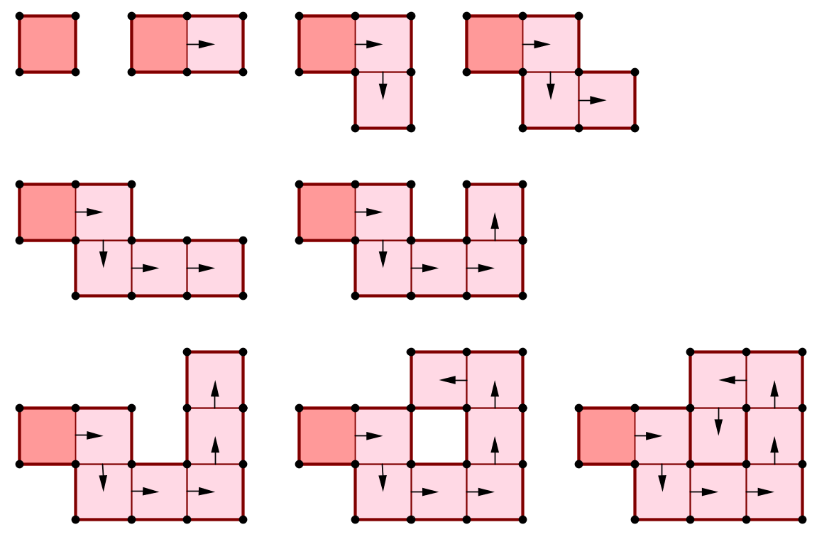
Figure 6: Frame Expansion: Example 1. Part I.

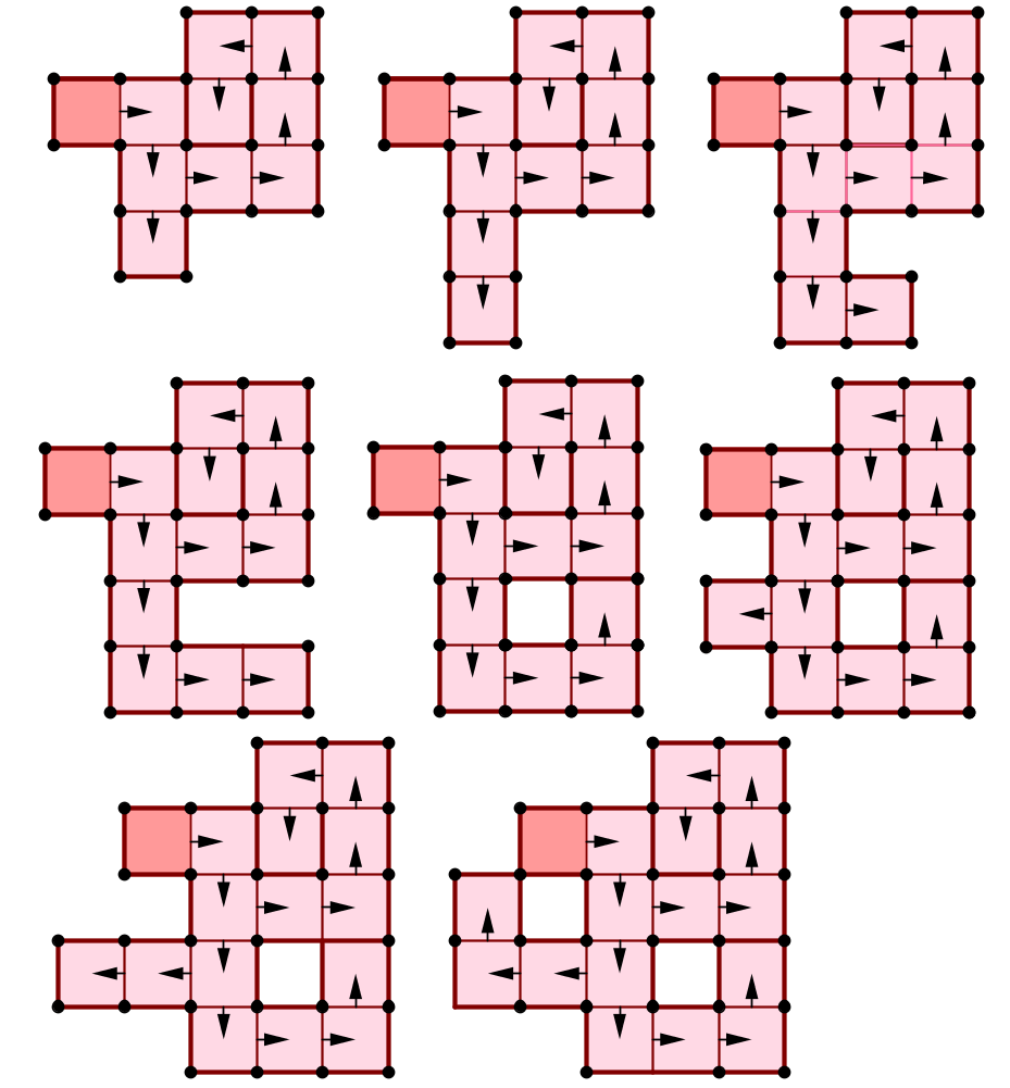
Figure 7: Frame Expansion: Example 1. Part II.

Figure 10: Frame Expansion: Example 2: Part III

Figure 11: Frame Expansion: Example 3: Part 1

Figure 12: Frame Expansion: Exampe 3: Part 2

10 Detailed Pseudocode

1:procedure calcHomology($\mathcal{M},\mathcal{A}$;)

2:   $\mathscr{V}\colonequals\textbf{mainFrame}(\mathcal{M})$;

3:   $\triangle_{c}\colonequals\textbf{calcbdryOp}(\mathcal{M},\mathcal{H},\mathscr{V})$;

4:   $H(\mathcal{M},\mathcal{A})\colonequals\textbf{SmithNormalForm}(\triangle_{c},\mathcal{A})$;

5:end procedure

6:

7:procedure calcBdryOp($\mathcal{M},\mathcal{H},\mathscr{V}$)

8:   $\textbf{topologicalSort}(\mathcal{H},\mathscr{V},\mathcal{L},\textsf{'ASCENDING')}$;

9:   for $1\leq i\leq\left\lvert\mathcal{L}\right\rvert$; $\sigma\colonequals\mathcal{L}[i]$ do

10:         if $\dim\sigma=0$ & $\sigma\raisebox{-1.07639pt}{\scalebox{1.2}{$\cdot$}}\textsf{pair}=\textsf{NIL}$ then

11:               $\triangle\sigma=\emptyset$;

12:         else if $\sigma\prec\beta$ & $\sigma\raisebox{-1.07639pt}{\scalebox{1.2}{$\cdot$}}\textsf{pair}=\beta$ then

13:               $\triangle\sigma=<\partial\beta,\sigma>\times\triangle\beta$;

14:         else

15:               Let $\tau_{i}\prec\sigma$ be the set of regular cells incident on $\sigma$ s.t. $\langle\tau_{i},\sigma\rangle\notin\mathscr{V}$;

16:               Let $\alpha_{i}\prec\sigma$ be the set of critical cells incident on $\sigma$;

17:               $\triangle\sigma=\sum\triangle\tau_{i}\times<\partial\sigma,\tau_{i}>+\sum\bm{\alpha_{i}}\times<\partial\sigma,\alpha_{i}>$;

18:         end if

19:         if $\sigma\raisebox{-1.07639pt}{\scalebox{1.2}{$\cdot$}}\textsf{pair}=\textsf{NIL}$ & $\sigma\raisebox{-1.07639pt}{\scalebox{1.2}{$\cdot$}}\textsf{revPair}=\textsf{NIL}$ then

20:               $\triangle_{c}\sigma\colonequals\triangle\sigma$;

21:         end if

22:   end for

23:end procedure

Algorithm 4 $\textbf{Homology}()$

1:procedure findCoBdry($\mathcal{M}^{d},\mathcal{B}^{d}$)

2:   Go through list $\mathcal{M}^{d}$. If $\mathcal{M}^{d}[i]$ has only one face, add $\mathcal{M}^{d}[i]$ to $\mathcal{B}$

3:   $\textbf{return }\mathcal{B}$;

4:end procedure

5:

6:procedure addPairToVectorField($\tau,\vartheta,\mathscr{V},\mathcal{M},\mathcal{B}^{d},d$)

7:   if $\tau\raisebox{-1.07639pt}{\scalebox{1.2}{$\cdot$}}\textsf{revPair}=\textsf{NIL}$ then

8:         $\textbf{delete}(\tau,\mathcal{M}^{d});\textbf{delete}(\vartheta,\mathcal{M}^{d-1})$;

9:         if $\tau\in\mathcal{B}$ then $\textbf{delete}(\tau,\mathcal{B})$; end if

10:         $\textbf{nQ}(\mathcal{Q},\tau)$; $\vartheta\raisebox{-1.07639pt}{\scalebox{1.2}{$\cdot$}}$ pair $\colonequals\tau$; $\tau\raisebox{-1.07639pt}{\scalebox{1.2}{$\cdot$}}$ revPair $\colonequals\vartheta$;

11:         $\mathscr{V}\colonequals\mathscr{V}+\langle\vartheta,\tau\rangle$

12:   end if

13:end procedure

14:

15:procedure frameFlow($\mathcal{M},d,\mathscr{V}$)

16:   if $(\varpi=\textbf{dQ}(\mathcal{B}^{d}))$ = NIL then

17:         $\varpi\colonequals\textbf{dQ}(\mathcal{M}^{d})$;

18:   end if

19:   repeat

20:         fF $\colonequals$ ’T’;

21:         repeat

22:               $\mathcal{F}\colonequals\textbf{faces}(\varpi)-\varpi\raisebox{-1.07639pt}{\scalebox{1.2}{$\cdot$}}\textsf{revPair}$; $\upsilon\colonequals\textbf{bdry}(\mathcal{F})$;

23:               if fF=’T’ & $\upsilon\neq$ NIL then

24:                     addPairToVectorField($\varpi,\upsilon,\mathscr{V},\mathcal{M},\mathcal{B}^{d},d$);

25:               else

26:                     $\textbf{delete}(\varpi,\mathcal{M}^{d})$;

27:               end if

28:               fF$\colonequals$’F’;

29:               for $1\leq i\leq\left\lvert\mathcal{F}\right\rvert$; do

30:                     $\vartheta\colonequals\mathcal{F}[i]$; $\mu\colonequals\textbf{cofaces}(\vartheta)-\varpi$;

31:                     $\textbf{addPairToVectorField}(\mu,\vartheta,\mathscr{V},\mathcal{M},\mathcal{B}^{d},d$);

32:               end for

33:         until $(\varpi=\textbf{dQ}(\mathcal{Q}))\neq\textsf{NIL}$

34:   until $(\varpi=\textbf{dQ}(\mathcal{B}^{d}))\neq\textsf{NIL}$

35:end procedure

36:

37:procedure mainFrame($\mathcal{M},\mathscr{V}$)

38:   $\mathcal{B}^{2}$ findCoBdry ($\mathcal{M}^{2}$);

39:    frameFlow ($\mathcal{M}$,2,$\mathcal{B}^{2}$,$\mathscr{V}$);

40:   $\left\{\mathcal{M}^{1}[1:\textsf{numEars}],\textsf{numEars}\right\}\colonequals\textbf{earDecompose}(\mathcal{M}$);

41:   for $1\leq i\leq\textsf{numEars}$ do

42:         $\mathcal{B}^{1}[i]\colonequals\textbf{findCoBdry}(\mathcal{M}^{1}[i]$);

43:          frameFlow ($\mathcal{M}^{1}[i]$,1,$\mathcal{B}^{1}[i]$,$\mathscr{V}$);

44:   end for

45:   $\textbf{return }\mathscr{V}$.;

46:end procedure

Algorithm 5 $\textsf{Algorithm }\textbf{FrameFlow}()$

References

- [1] Ayala, R., Fernández-Ternero, D., and Vilches, J. A. A graph-theoretical approach to cancelling critical elements. Elec. Notes in Dis. Math. 37, 285-290 (2011).
- [2] Ayala, R., Fernández-Ternero, D., and Vilches, J. A. Perfect discrete morse functions on 2-complexes. Pattern Recognition Letters 33(11) (2012).
- [3] Bauer, U., Lange, C., and Wardetzky, M. Optimal topological simplification of discrete functions on surfaces. Discrete & Computational Geometry 47, 2 (2012), 347–377.
- [4] Benedetti, B., and Lutz, F. H. Random discrete morse theory and a new library of triangulations. CoRR abs/1303.6422 (2013).
- [5] Burton, B. A., Lewiner, T., Paixão, J., and Spreer, J. Parameterized complexity of discrete morse theory. CoRR abs/1303.7037 (2013).
- [6] Forman, R. Morse theory for cell complexes. Advances in Mathematics 134, 1 (Mar. 1998), 90–145.
- [7] Forman, R. A user’s guide to discrete Morse theory. Séminaire Lotharingien de Combinatoire B48c (2002), 1–35.
- [8] Harker, S., Mischaikow, K., Mrozek, M., Nanda, V., Wagner, H., Juda, M., and Dlotko, P. The efficiency of a homology algorithm based on discrete morse theory and coreductions. In Proc. of 3rd Intl. Workshop on CTIC (2010), vol. 1(1).
- [9] Hersh, P. On optimizing discrete Morse functions. Advances in Applied Mathematics 35, 3 (Sept. 2005), 294–322.
- [10] Joswig, M., and Pfetsch, M. Computing optimal discrete morse functions. SIAM J. Discrete Math. 20, 1 (2004), 11–25.
- [11] Juda, M., and Mrozek, M. Z2-homology of weak 2-pseudomanifolds may be computed in o(nlogn) time. preprint (2009).
- [12] Lee, J. M. Introduction to topological manifolds : with 138 illustrations. Graduate texts in mathematics. Springer, New York, Berlin, Heidelberg, 2000.
- [13] Lewiner, T. Constructing discrete morse functions. Master’s thesis, Department of Mathematics, PUC-Rio, july 2002.
- [14] Lewiner, T., Lopes, H., and Tavares, G. Optimal discrete morse functions for 2-manifolds. Comput. Geom. 26, 3 (2003), 221–233.
- [15] Lewiner, T., Lopes, H., and Tavares, G. Toward optimality in discrete morse theory. Experimental Mathematics 12, 3 (2003), 271–285.
- [16] Matsumoto, Y. An Introduction to Morse theory. AMS, Providence, 2002.
- [17] Milnor, J. Morse Theory, 1st edition ed. Princeton University Press, May 1963.
- [18] Rathore, A. Min morse: Approximability & applications. CoRR abs/1503.03170 (2015).