Reaction rates of ⁶⁴Ge($p$,$\gamma$)⁶⁵As and ⁶⁵As($p$,$\gamma$)⁶⁶Se and the extent of nucleosynthesis in type I X-ray bursts

Abstract

The extent of nucleosynthesis in models of type I X-ray bursts and the associated impact on the energy released in these explosive events are sensitive to nuclear masses and reaction rates around the ⁶⁴Ge waiting point. Using the well known mass of ⁶⁴Ge, the recently measured ⁶⁵As mass, and large-scale shell model calculations, we have determined new thermonuclear rates of the ⁶⁴Ge($p$,$\gamma$)⁶⁵As and ⁶⁵As($p$,$\gamma$)⁶⁶Se reactions with reliable uncertainties. The new reaction rates differ significantly from previously published rates. Using the new data we analyze the impact of the new rates and the remaining nuclear physics uncertainties on the ⁶⁴Ge waiting point in a number of representative one-zone X-ray burst models. We find that in contrast to previous work, when all relevant uncertainties are considered, a strong ⁶⁴Ge $rp$-process waiting point cannot be ruled out. The nuclear physics uncertainties strongly affect X-ray burst model predictions of the synthesis of ⁶⁴Zn, the synthesis of nuclei beyond $A=64$, energy generation, and burst light curve. We also identify key nuclear uncertainties that need to be addressed to determine the role of the ⁶⁴Ge waiting point in X-ray bursts. These include the remaining uncertainty in the ⁶⁵As mass, the uncertainty of the ⁶⁶Se mass, and the remaining uncertainty in the ⁶⁵As($p$,$\gamma$)⁶⁶Se reaction rate, which mainly originates from uncertain resonance energies.

1. Introduction

A type I X-ray burst (XRB) arises from a thermonuclear runaway in the accreted envelope of a neutron star in a close binary star system (for reviews, see, e.g., Lewin et al. (1993); Schatz et al. (1998); Strohmayer & Bildsten (2006); Parikh et al. (2013)). Roughly 100 bursting systems have been discovered to date, with light curves exhibiting peak luminosities of $L_{\mathrm{peak}}\approx$ 10⁴–10⁵ $L_{\mathrm{\odot}}$ and timescales of 10–100 s. During an XRB, models predict that a H/He-rich accreted envelope may become strongly enriched in heavier nuclei though the $\alpha$$p$-process and the $rp$-process (Wallace & Woosley, 1981; Schatz et al., 1998). These two processes involve $\alpha$-particle-induced or proton-capture reactions on stable and radioactive nuclei, interrupted by occasional $\beta$-decays. When the $rp$-process approaches the proton dripline, successive capture of protons by nuclei is inhibited by a strong reverse photodisintegration reaction rate. The competition between the rate of proton capture and the rate of $\beta$-decay at these “waiting points” (e.g., ⁶⁰Zn, ⁶⁴Ge, and ⁶⁸Se) determines the extent of the synthesis of heavier mass nuclei during the burst (Schatz et al., 1998). Peak temperatures during the thermonuclear runaway may approach or exceed 1 GK, resulting in the synthesis of nuclei up to mass $A\approx 100$ (Schatz et al., 2001; Elomaa et al., 2009). Model predictions depend, however, on astrophysical parameters such as accretion rate, the composition of the accreted material, and the neutron star surface gravity, as well as on nuclear physics quantities such as nuclear masses and reaction rates.

The ⁶⁴Ge($p$,$\gamma$)⁶⁵As and ⁶⁵As($p$,$\gamma$)⁶⁶Se reactions have been demonstrated to have a significant impact on nucleosynthesis during XRBs. (See Parikh et al. (2014) for a recent review of the impact of nuclear physics uncertainties on predicted yields and light curves from XRB models.) Direct measurements of these reactions at the relevant energies in XRBs are not yet possible due to the lack of sufficiently intense radioactive ⁶⁴Ge and ⁶⁵As beams. Moreover, due to the unknown mass of ⁶⁶Se and the lack of nuclear structure information for states within $\approx$ 1–2 MeV of the ⁶⁴Ge+$p$ and the (theoretical) ⁶⁵As+$p$ energy thresholds in ⁶⁵As and ⁶⁶Se, respectively, it is not possible to estimate rates for these reactions based on experimental nuclear structure data. As a result, XRB models use ⁶⁴Ge($p$,$\gamma$)⁶⁵As and ⁶⁵As($p$,$\gamma$)⁶⁶Se thermonuclear rates derived from theoretical calculations. Using such models it has been demonstrated that varying the ⁶⁵As($p$,$\gamma$)⁶⁶Se rate by a factor of ten at the relevant temperatures affects the calculated abundances of nuclei between $A\approx$ 65–100 by factors as large as about 5 (Parikh et al., 2008). For ⁶⁴Ge($p$,$\gamma$)⁶⁵As, models have illustrated the importance of the $Q$-value (or proton separation energy $S_{p}$) adopted for this reaction, with variations by $\pm$300 keV affecting final calculated abundances between $A\approx$ 65–100 by factors as large as about 5 (Parikh et al., 2008, 2009). In addition, the effective $rp$-process lifetime of the waiting-point nucleus ⁶⁴Ge was investigated by Schatz (2006) based on the estimated proton separation energies of $S_{p}$(⁶⁵As)=-0.36$\pm$0.15 MeV and $S_{p}$(⁶⁶Se)=2.43$\pm$0.18 MeV, derived from Coulomb mass shift calculations (Brown et al., 2002). It was found that the effective lifetime of ⁶⁴Ge for a given temperature and proton density is mainly determined by the $S_{p}$ values of ⁶⁵As and ⁶⁶Se and the proton capture rate on ⁶⁵As.

Recently, precise mass measurements of nuclei along the $rp$-process path have become available. The mass of ⁶⁴Ge has been measured at the Canadian Penning Trap at Argonne National Laboratory (Clark et al., 2007) and the LEBIT Penning Trap facility at Michigan State University (Schury et al., 2007). More recently, the mass of ⁶⁵As has been measured at the HIRFL-CSR (Cooler-Storage Ring at the Heavy Ion Research Facility in Lanzhou) (Xia et al., 2002) using IMS (Isochronous Mass Spectrometry). The measurements can be combined to obtain an experimental proton separation energy for ⁶⁵As of $S_{p}=-90\pm 85$ keV (Tu et al., 2011), where the uncertainty is dominated by the uncertainty in the ⁶⁵As mass. The mass of ⁶⁶Se is not known experimentally. The extrapolated value predicted by AME2012 results in $S_{\rm p}(^{66}$Se$)=1720\pm 310$ keV. With the new mass of ⁶⁵As, X-ray burst model calculations (Tu et al., 2011) suggested that ⁶⁴Ge may not be a significant $rp$-process waiting point, contrary to previous expectations (Schatz et al., 1998; Woosley et al., 2004; Fisker et al., 2008; Parikh et al., 2009; José et al., 2010). We revisit this question here using our new nuclear reaction rates.

Thermonuclear ⁶⁴Ge($p$,$\gamma$) and ⁶⁵As($p$,$\gamma$) reaction rates were first estimated by Van Wormer et al. (1994) based entirely on the properties of the mirror nuclei ⁶⁵Ge and ⁶⁶Ge, respectively. $S_{p}$ values of ⁶⁵As and ⁶⁶Se were estimated to be 0.169 MeV and 1.909 MeV, respectively. Later on, both rates have been calculated (Rauscher & Thielemann, 2000) with the statistical Hauser-Feshbach formalism (NON-SMOKER (Rauscher & Thielemann, 1998)) using the masses of ⁶⁵As and ⁶⁶Se predicted by the finite-range droplet (FRDM) (Möller et al., 1995) and ETSFIQ (Pearson et al., 1996) mass models. Recently, the statistical model calculations have been updated using new predictions for the ⁶⁵As and ⁶⁶Se proton separation energies (see JINA REACLIB (Cyburt et al., 2010)). The predicted rates differ from one another by up to several orders of magnitude over typical XRB temperatures. Moreover, the reliability of statistical model calculations for these rates is questionable due to the low compound nucleus level densities, especially for ⁶⁴Ge($p$,$\gamma$), but also for ⁶⁵As($p$,$\gamma$).

In this work we refer to previously available rates using the nomenclature adopted in the JINA REACLIB database. The laur rate refers to the rate estimated by Van Wormer et al. (1994); the rath rate was calculated by Rauscher & Thielemann (2000). The rath, thra, rpsm rates are the statistical-model calculations with FRDM, ETSFIQ, as well as Audi & Wapstra (1995) estimated masses, respectively. The recent ths8 rate is from Cyburt et al. (2010).

Here we determine new thermonuclear ⁶⁴Ge($p$,$\gamma$)⁶⁵As and ⁶⁵As($p$,$\gamma$)⁶⁶Se reaction rates using the updated $S_{p}$ values of ⁶⁵As and ⁶⁶Se together with new nuclear structure information from large-scale shell-model calculations. Using the new data we fully characterize the nuclear physics uncertainties that affect the $rp$-process through ⁶⁴Ge and reexamine the question of the ⁶⁴Ge waiting point.

2. Reaction rate calculations

The total thermonuclear proton capture reaction rate consists of the sum of resonant- and direct-capture (DC) on ground state and thermally excited states in the target nucleus, weighted with their individual population factors (Fowler et al., 1964; Rolfs & Rodney, 1988). It can be calculated by the following equation:

$$N_{A}\langle\sigma v\rangle=\sum_{i}(N_{A}\langle\sigma v\rangle_{r}^{i}+N_{A}\langle\sigma v\rangle_{\mathrm{DC}}^{i})\frac{(2J_{i}+1)e^{-E_{i}/kT}}{\sum_{n}(2J_{n}+1)e^{-E_{n}/kT}}$$

(1)

with the parameters defined by Schatz et al. (2005).

2.1. Resonant rates

For isolated narrow resonances, the resonant reaction rate for capture on a nucleus in an initial state $i$, $N_{A}\langle\sigma v\rangle_{r}^{i}$, can be calculated as a sum over all relevant compound nucleus states $j$ above the proton threshold (Rolfs & Rodney, 1988; Iliadis, 2007). It can be expressed by the following equation (Schatz et al., 2005):

$$N_{A}\langle\sigma v\rangle_{r}^{i}= 1.54\times 10^{11}(\mu T_{9})^{-3/2}$$

$$\times\sum_{j}\omega\gamma_{ij}\mathrm{exp}\left(-\frac{11.605E_{ij}}{T_{9}}\right)[\mathrm{cm^{3}s^{-1}mol^{-1}}],$$

where the resonance energy in the center-of-mass system, $E_{ij}=E_{j}-S_{p}-E_{i}$, is calculated from the excitation energies of the initial $E_{i}$ and compound nucleus $E_{j}$ state. For the ground-state capture, the resonance energy is represented by $E_{r}^{i}=E_{x}^{j}-S_{p}$. $T_{9}$ is the temperature in Giga Kelvin (GK) and $\mu$ is the reduced mass of the entrance channel in atomic mass units ($\mu=A_{T}/(1+A_{T})$, with $A_{T}$ the target mass number). In Eq. LABEL:eq2, the resonance energy and strength are in units of MeV. The resonance strength $\omega\gamma$ is defined by

$$\omega\gamma_{ij}=\frac{2J_{j}+1}{2(2J_{i}+1)}\frac{\Gamma_{p}^{ij}\times\Gamma_{\gamma}^{j}}{\Gamma_{\mathrm{total}}^{j}}.$$ (3)

where $J_{i}$ is the target spin and $J_{j}$, $\Gamma_{p}^{ij}$ , $\Gamma_{\gamma}^{j}$, and $\Gamma_{\mathrm{total}}^{j}$ are spin, proton decay width, $\gamma$-decay width, and total width of the compound nucleus state $j$, respectively. The total width is given by $\Gamma_{\mathrm{total}}^{j}=\Gamma_{\gamma}^{j}+\sum_{i}\Gamma_{p}^{ij}$, because other decay channels are closed (Audi et al., 2012) in the excitation energy range considered in this work.

Table 1Properties of ⁶⁵As for the ground-state capture utilized in the present ⁶⁴Ge($p$,$\gamma$)⁶⁵As resonant rate calculation. The energy levels in the mirror nucleus ⁶⁵Ge are listed in the 4^th column for comparison.

$J^{\pi}_{i}$[a]	$E_{x}$ [MeV]			$E_{r}$ (MeV)[d]	$nlj$	$C^{2}S$	$\Gamma_{p}$ [eV]	$\Gamma_{\gamma}$ [eV]	$\omega\gamma$ [eV]
	$E^{\mathrm{exp}}_{x}$[a]	$E^{\mathrm{theo}}_{x}$[b]	$E_{x}$(65Ge)[c]
3/2${}^{-}_{1}$	0.000	0.000	0.000	0.090	2$p_{3/2}$	0.196	$1.19\times 10^{-34}$	0.00	0.00
5/2${}^{-}_{1}$[e]	0.187(3)	0.103	0.111	0.277	1$f_{5/2}$	0.533	$8.19\times 10^{-17}$	5.11$\times$10-7	2.46$\times$10-16
5/2${}^{-}_{2}$		0.501	0.605	0.591	1$f_{5/2}$	0.010	$3.76\times 10^{-10}$	4.73$\times$10-5	1.13$\times$10-9
5/2${}^{-}_{3}$		0.863		0.953	1$f_{5/2}$	0.014	$1.64\times 10^{-6}$	4.24$\times$10-4	4.89$\times$10-6
7/2${}^{-}_{1}$		0.947	0.890	1.037	1$f_{7/2}$	0.013	$1.28\times 10^{-5}$	2.43$\times$10-4	4.88$\times$10-5
7/2${}^{-}_{2}$[f]		1.070	1.155	1.160	1$f_{7/2}$	0.002	$8.50\times 10^{-6}$	2.11$\times$10-4	3.27$\times$10-5

$[\textnormal{a}]$ measured by Obertelli et al. (2011);

$[\textnormal{b}]$ calculated by the present shell model;

$[\textnormal{c}]$ compiled by Browne & Tuli (2010);

$[\textnormal{d}]$ calculated by $E_{r}=E_{x}-S_{p}$ with $S_{p}=-0.09$ MeV (Tu et al., 2011);

$[\textnormal{e}]$ calculated $E_{r}$ and $\Gamma_{p}$ based on the experimental value of $E_{x}=0.187$ MeV for this state;

$[\textnormal{f}]$ negligible contribution to the rate for temperatures up to 2 GK.

The proton width can be estimated by the following equation,

$$\Gamma_{p}=\sum_{nlj}C^{2}S(nlj)\,\Gamma_{sp}(nlj)\,,$$ (4)

where $C^{2}S(nlj)$ denotes a proton-transfer spectroscopic factor, while $\Gamma_{sp}$ is a single-proton width for capture of a proton on an $(nlj)$ quantum orbital. The $\Gamma_{sp}$ are obtained from proton scattering cross sections calculated with a Woods-Saxon potential (Richter et al., 2011; Brown, 2014). Alternatively, the proton partial widths may also be calculated by the following expression (Van Wormer et al., 1994; Herndl et al., 1995),

$$\Gamma_{p}=\frac{3\hbar^{2}}{\mu R^{2}}P_{\ell}(E)C^{2}S.$$ (5)

Here, $R=r_{0}\times(1+A_{T})^{1/3}$ fm (with $r_{0}=1.25$ fm) is the nuclear channel radius. The Coulomb penetration factor $P_{\ell}$ is given by

$$P_{\ell}(E)=\frac{kR}{F^{2}_{\ell}(E)+G^{2}_{\ell}(E)},$$ (6)

where $k=\sqrt{2\mu E}/\hbar$ is the wave number with energy $E$ in the center-of-mass (c.m.) system; $F_{\ell}$ and $G_{\ell}$ are the regular and irregular Coulomb functions, respectively. The proton widths given by these two methods (i.e., by Eqs. 4 and 5) agree well with each other, with a maximum difference of about 35%.

The key ingredients necessary to estimate the resonant ⁶⁴Ge($p$,$\gamma$) and ⁶⁵As($p$,$\gamma$) rates are energy levels in ⁶⁵As and ⁶⁶Se, proton transfer spectroscopic factors, and proton and gamma-ray partial widths. For ⁶⁵As, only a single level has been observed at $E_{x}=187(3)$ keV (Obertelli et al., 2011). For ⁶⁶Se, one level has been confirmed at $E_{x}=929(7)$ keV, and indications for two other levels at 2064(3) keV and 3520(4) keV have been reported, with tentative assignments of (4⁺) and (6⁺), respectively (Obertelli et al., 2011; Ruotsalainen et al., 2013). There are no more experimental data available for these two nuclei. In this work, we have calculated the energy levels, spectroscopic factors and gamma widths within the framework of a large-scale shell model, without truncation, using the shell-model code NuShellX@MSU (Brown & Rae, 2014). The effective interaction GXPF1a (Honma et al., 2004, 2005) has been utilized for these two pf-shell nuclei.

The $\gamma$ widths, $\Gamma_{\gamma}$, have been calculated from the electromagnetic reduced transition probabilities $B$($J_{i}\rightarrow J_{f};L$), which carry the nuclear structure information of the resonant states and the final bound states (Brussaard & Glaudemans, 1977). The reduced transition rates are computed within the shell model. Most of the transitions in this work are of $M1$ and $E2$ types. The relations are (Herndl et al., 1995):

$$\Gamma_{E2}\mathrm{[eV]}=8.13\times 10^{-7}E_{\gamma}^{5}\mathrm{[MeV]}B(E2)\mathrm{[e^{2}fm^{4}]},$$ (7)

and

$$\Gamma_{M1}\mathrm{[eV]}=1.16\times 10^{-2}E_{\gamma}^{3}\mathrm{[MeV]}B(M1)\mathrm{[\mu_{N}^{2}]}.$$ (8)

The $B(E2)$ values have been obtained from empirical effective charges, $e_{p}=1.5e$, $e_{n}=0.5e$, whereas the $B(M1)$ values have been obtained with a four-parameter set of empirical $g$-factors, i.e. $g^{s}_{p}=5.586$, $g^{s}_{n}=-3.826$ and $g^{l}_{p}=1$, $g^{l}_{n}=0$ (Honma et al., 2004).

In addition, we have also included proton resonant captures on the thermally excited target states. Since the first-excited state in ⁶⁴Ge is quite high ($E_{x}=902$ keV), thermal excitation can be neglected for typical X-ray burst temperatures. For the ⁶⁵As($p$,$\gamma$)⁶⁶Se rate, we included proton capture on the first four thermally excited states of ⁶⁵As (i.e., on the 0.187, 0.501, 0.863 and 0.947 MeV states listed in Table 1). Capture on thermally excited states contributes at most 38% to the total capture rate at 2 GK (Lam et al., 2016). The properties of ⁶⁵As and ⁶⁶Se for the ground-state captures are summarized in Table 1 and Table 2, respectively. In addition, the properties of ⁶⁶Se for the first-excited-state capture (the major thermally excited-state contribution) are summarized in Table 3.

Table 2Properties of ⁶⁶Se for the ground-state capture utilized in the present ⁶⁵As($p$,$\gamma$)⁶⁶Se resonant rate calculation.

$J^{\pi}_{i}$[a]	$E_{x}$ [MeV]		$E_{r}$ [MeV][c]	$C^{2}S_{7/2}$	$C^{2}S_{3/2}$	$C^{2}S_{5/2}$	$C^{2}S_{1/2}$	$\Gamma_{\gamma}$ [eV]	$\Gamma_{p}$ [eV]	$\omega\gamma$ [eV]
	$E_{x}^{\mathrm{exp}}$[b]	$E_{x}^{\mathrm{theo}}$[a]		$(l=3)$	$(l=1)$	$(l=3)$	$(l=1)$
${0}^{+}_{1}$	0.000	0.000	—		0.746			—	—	—
${2}^{+}_{1}$	0.929(7)	0.982	—	$0.037$	$0.069$	$0.119$	$0.045$	$2.765\times 10^{-4}$	—	—
${0}^{+}_{2}$		1.130	—		0.013			$2.020\times 10^{-8}$	—	—
${2}^{+}_{2}$		1.552	—	$0.002$	$0.011$	$0.071$	$0.051$	$1.402\times 10^{-4}$	—	—
${0}^{+}_{3}$		1.575	—		$0.002$			$2.056\times 10^{-6}$	—	—
${2}^{+}_{3}$		1.952	0.232	$0.001$	$0.001$	$0.180$	$0.000$	$4.040\times 10^{-4}$	$3.079\times 10^{-20}$	$1.924\times 10^{-20}$
${0}^{+}_{4}$		1.989	0.269		$0.002$			$1.441\times 10^{-8}$	$4.797\times 10^{-18}$	$5.996\times 10^{-19}$
${2}^{+}_{4}$		2.053	0.333[e]	$0.002$	$0.005$	$0.027$	$0.025$	$2.218\times 10^{-4}$	$3.517\times 10^{-14}$	$2.198\times 10^{-14}$
${4}^{+}_{1}$	2.064(3)[d]	2.110	0.344	$0.008$		$0.004$		$8.382\times 10^{-4}$	$2.301\times 10^{-16}$	$2.589\times 10^{-16}$
${3}^{+}_{1}$		2.102	0.382	$0.001$	$0.000$	$0.017$		$3.835\times 10^{-5}$	$1.057\times 10^{-14}$	$9.249\times 10^{-15}$
${2}^{+}_{5}$		2.277	0.557[e]	$0.000$	$0.004$	$0.015$	$0.001$	$1.751\times 10^{-4}$	$2.205\times 10^{-9}$	$1.378\times 10^{-9}$
${3}^{+}_{2}$		2.419	0.699	$0.000$	$0.004$	$0.063$		$2.361\times 10^{-4}$	$1.781\times 10^{-7}$	$1.557\times 10^{-7}$
${1}^{+}_{1}$		2.474	0.754[e]		$0.016$	$0.000$	$0.052$	$3.579\times 10^{-3}$	$1.152\times 10^{-5}$	$4.306\times 10^{-6}$
${4}^{+}_{2}$		2.498	0.778	$0.001$		$0.115$		$2.653\times 10^{-4}$	$1.888\times 10^{-7}$	$2.122\times 10^{-7}$
${2}^{+}_{6}$		2.556	0.836[e]	$0.001$	$0.021$	$0.033$	$0.032$	$9.915\times 10^{-4}$	$6.723\times 10^{-5}$	$3.935\times 10^{-5}$
${3}^{+}_{3}$		2.668	0.948	$0.000$	$0.065$	$0.145$		$1.550\times 10^{-4}$	$7.969\times 10^{-4}$	$1.136\times 10^{-4}$
${4}^{+}_{3}$		2.740	1.020	$0.002$		$0.040$		$8.404\times 10^{-4}$	$8.287\times 10^{-6}$	$9.232\times 10^{-6}$
${1}^{+}_{2}$		2.781	1.061[e]		$0.060$	$0.351$	$0.002$	$5.338\times 10^{-3}$	$4.483\times 10^{-3}$	$9.137\times 10^{-4}$
${2}^{+}_{7}$		2.865	1.145	$0.000$	$0.000$	$0.000$	$0.028$	$1.175\times 10^{-3}$	$5.315\times 10^{-3}$	$6.014\times 10^{-4}$
${1}^{+}_{3}$		2.867	1.147		$0.065$	$0.001$	$0.222$	$2.170\times 10^{-3}$	$5.887\times 10^{-2}$	$7.847\times 10^{-4}$
${3}^{+}_{4}$		2.882	1.162	$0.002$	$0.003$	$0.002$		$1.209\times 10^{-3}$	$9.439\times 10^{-4}$	$4.639\times 10^{-4}$
${0}^{+}_{5}$		2.888	1.168		$0.629$			$1.716\times 10^{-4}$	$1.985\times 10^{-1}$	$2.143\times 10^{-5}$
${4}^{+}_{4}$		2.907	1.187	$0.000$		$0.005$		$3.139\times 10^{-4}$	$1.001\times 10^{-5}$	$1.091\times 10^{-5}$
${2}^{+}_{8}$		2.949	1.229	$0.000$	$0.003$	$0.005$	$0.016$	$9.006\times 10^{-4}$	$1.085\times 10^{-2}$	$5.197\times 10^{-4}$
${3}^{+}_{5}$		2.969	1.249	$0.000$	$0.006$	$0.000$		$7.804\times 10^{-4}$	$4.817\times 10^{-3}$	$5.877\times 10^{-4}$
${4}^{+}_{5}$		2.998	1.278	$0.000$		$0.079$		$1.392\times 10^{-3}$	$4.711\times 10^{-4}$	$3.960\times 10^{-4}$
${4}^{+}_{6}$		3.114	1.394	$0.000$		$0.157$		$1.374\times 10^{-3}$	$3.262\times 10^{-3}$	$1.088\times 10^{-3}$
${2}^{+}_{9}$		3.217	1.497	$0.000$	$0.003$	$0.021$	$0.036$	$1.534\times 10^{-3}$	$3.221\times 10^{-1}$	$9.539\times 10^{-4}$
${0}^{+}_{6}$		3.231	1.511		$0.002$			$2.561\times 10^{-3}$	$2.244\times 10^{-2}$	$2.873\times 10^{-4}$
${3}^{+}_{6}$		3.237	1.517	$0.000$	$0.000$	$0.006$		$1.586\times 10^{-3}$	$5.258\times 10^{-3}$	$1.066\times 10^{-3}$
${1}^{+}_{4}$		3.274	1.554		$0.005$	$0.072$	$0.010$	$3.113\times 10^{-3}$	$2.111\times 10^{-1}$	$1.151\times 10^{-3}$
${4}^{+}_{7}$		3.299	1.579	$0.000$		$0.008$		$9.407\times 10^{-4}$	$1.075\times 10^{-3}$	$5.644\times 10^{-4}$
${3}^{+}_{7}$		3.328	1.608	$0.001$	$0.004$	$0.022$		$1.139\times 10^{-3}$	$8.762\times 10^{-2}$	$9.842\times 10^{-4}$
${2}^{+}_{10}$		3.330	1.610	$0.008$	$0.083$	$0.001$	$0.012$	$2.089\times 10^{-3}$	$2.222\times 10^{+0}$	$1.304\times 10^{-3}$
${2}^{+}_{11}$		3.357	1.637	$0.001$	$0.000$	$0.027$	$0.114$	$1.348\times 10^{-3}$	$2.761\times 10^{+0}$	$8.423\times 10^{-4}$
${5}^{+}_{1}$		3.394	1.674	$0.000$				$1.355\times 10^{-3}$	$1.460\times 10^{-4}$	$1.812\times 10^{-4}$
${4}^{+}_{8}$		3.424	1.704	$0.000$		$0.018$		$1.417\times 10^{-3}$	$5.639\times 10^{-3}$	$1.274\times 10^{-3}$
${3}^{+}_{8}$		3.487	1.767	$0.000$	$0.000$	$0.056$		$4.881\times 10^{-3}$	$2.792\times 10^{-2}$	$3.635\times 10^{-3}$
${2}^{+}_{12}$		3.499	1.779	$0.006$	$0.060$	$0.001$	$0.041$	$4.335\times 10^{-4}$	$7.440\times 10^{+0}$	$2.709\times 10^{-4}$

$[\textnormal{a}]$calculated by the present shell model;

$[\textnormal{b}]$measured by Obertelli et al. (2011) and Ruotsalainen et al. (2013);

$[\textnormal{c}]$calculated by $E_{r}=E_{x}-S_{p}$ with $S_{p}=1.720$ MeV (AME2012);

$[\textnormal{d}]$calculated $E_{r}$ and $\Gamma_{p}$ based on the experimental value of $E_{x}=2.064$ MeV for this state;

$[\textnormal{e}]$resonances dominantly contributing to the rate within temperature region of 0.2–2 GK.

Table 3Properties of ⁶⁶Se for the first-excited-state capture utilized in the present ⁶⁵As${}^{5/2_{1}^{-}}$($p$,$\gamma$)⁶⁶Se resonant rate.

$J^{\pi}_{i}$[a]	$E_{x}$ [MeV]		$E_{r}$ [MeV][c]	$C^{2}S_{7/2}$	$C^{2}S_{3/2}$	$C^{2}S_{5/2}$	$C^{2}S_{1/2}$	$\Gamma_{\gamma}$ [eV]	$\Gamma_{p}$ [eV]	$\omega\gamma$ [eV]
	$E_{x}^{\mathrm{exp}}$[b]	$E_{x}^{\mathrm{theo}}$[a]		$(l=3)$	$(l=1)$	$(l=3)$	$(l=1)$
${2}^{+}_{3}$		1.952	0.045	0.002	0.035	0.000	0.013	$4.040\times 10^{-4}$	$4.401\times 10^{-56}$	$1.834\times 10^{-56}$
${0}^{+}_{4}$		1.989	0.082			0.244		$1.441\times 10^{-8}$	$2.398\times 10^{-40}$	$1.998\times 10^{-41}$
${2}^{+}_{4}$		2.053	0.146	0.000	0.019	0.088	0.098	$2.218\times 10^{-4}$	$4.499\times 10^{-26}$	$1.875\times 10^{-26}$
${4}^{+}_{1}$	2.064(3)[d]	2.110	0.157	0.001	0.016	0.002		$8.382\times 10^{-4}$	$1.261\times 10^{-25}$	$9.458\times 10^{-26}$
${3}^{+}_{1}$		2.102	0.195	0.001	0.011	0.000	0.001	$3.835\times 10^{-5}$	$4.039\times 10^{-22}$	$2.356\times 10^{-22}$
${2}^{+}_{5}$		2.277	0.370	0.001	0.038	0.020	0.184	$1.751\times 10^{-4}$	$4.549\times 10^{-12}$	$1.895\times 10^{-12}$
${3}^{+}_{2}$		2.419[e]	0.512	0.001	0.083	0.004	0.226	$2.361\times 10^{-4}$	$1.862\times 10^{-8}$	$1.086\times 10^{-8}$
${1}^{+}_{1}$		2.474	0.567	0.000	0.000	0.002		$3.579\times 10^{-3}$	$5.149\times 10^{-11}$	$1.287\times 10^{-11}$
${4}^{+}_{2}$		2.498	0.591	0.000	0.043	0.208		$2.653\times 10^{-4}$	$6.133\times 10^{-8}$	$4.599\times 10^{-8}$
${2}^{+}_{6}$		2.556	0.649	0.001	0.026	0.191	0.008	$9.915\times 10^{-4}$	$3.292\times 10^{-7}$	$1.371\times 10^{-7}$
${3}^{+}_{3}$		2.668[e]	0.761	0.004	0.107	0.000	0.002	$1.550\times 10^{-4}$	$2.983\times 10^{-5}$	$1.459\times 10^{-5}$
${4}^{+}_{3}$		2.740	0.833	0.002	0.011	0.001		$8.404\times 10^{-4}$	$1.353\times 10^{-5}$	$9.987\times 10^{-6}$
${1}^{+}_{2}$		2.781	0.874	0.001	0.032	0.002		$5.338\times 10^{-3}$	$9.809\times 10^{-5}$	$2.408\times 10^{-5}$
${2}^{+}_{7}$		2.865[e]	0.958	0.000	0.002	0.324	0.054	$1.175\times 10^{-3}$	$6.788\times 10^{-4}$	$1.793\times 10^{-4}$
${1}^{+}_{3}$		2.867	0.960	0.000	0.000	0.004		$2.170\times 10^{-3}$	$2.502\times 10^{-7}$	$6.254\times 10^{-8}$
${3}^{+}_{4}$		2.882[e]	0.975	0.001	0.008	0.001	0.035	$1.209\times 10^{-3}$	$7.087\times 10^{-4}$	$2.607\times 10^{-4}$
${0}^{+}_{5}$		2.888	0.981			0.089		$1.716\times 10^{-4}$	$8.636\times 10^{-6}$	$6.852\times 10^{-7}$
${4}^{+}_{4}$		2.907	1.000	0.000	0.000	0.518		$3.139\times 10^{-4}$	$6.881\times 10^{-5}$	$4.233\times 10^{-5}$
${2}^{+}_{8}$		2.949	1.042	0.000	0.006	0.012	0.007	$9.006\times 10^{-4}$	$6.740\times 10^{-4}$	$1.606\times 10^{-4}$
${3}^{+}_{5}$		2.969[e]	1.062	0.002	0.003	0.001	0.025	$7.804\times 10^{-4}$	$1.754\times 10^{-3}$	$3.151\times 10^{-4}$
${4}^{+}_{5}$		2.998[e]	1.091	0.003	0.025	0.000		$1.392\times 10^{-3}$	$2.795\times 10^{-3}$	$6.970\times 10^{-4}$
${4}^{+}_{6}$		3.114[e]	1.207	0.001	0.061	0.103		$1.374\times 10^{-3}$	$3.138\times 10^{-2}$	$9.872\times 10^{-4}$
${2}^{+}_{9}$		3.217	1.310	0.000	0.019	0.016	0.001	$1.534\times 10^{-3}$	$3.314\times 10^{-2}$	$6.107\times 10^{-4}$
${0}^{+}_{6}$		3.231	1.324			0.025		$2.561\times 10^{-3}$	$2.545\times 10^{-4}$	$1.929\times 10^{-5}$
${3}^{+}_{6}$		3.237	1.330	0.001	0.007	0.000	0.053	$1.586\times 10^{-3}$	$1.026\times 10^{-1}$	$9.112\times 10^{-4}$
${1}^{+}_{4}$		3.274	1.367	0.002	0.002	0.002		$3.113\times 10^{-3}$	$4.840\times 10^{-3}$	$4.737\times 10^{-4}$
${4}^{+}_{7}$		3.299	1.392	0.000	0.003	0.026		$9.407\times 10^{-4}$	$1.039\times 10^{-2}$	$6.470\times 10^{-4}$
${3}^{+}_{7}$		3.328	1.421	0.001	0.073	0.003	0.019	$1.139\times 10^{-3}$	$4.284\times 10^{-1}$	$6.629\times 10^{-4}$
${2}^{+}_{10}$		3.330	1.423	0.000	0.015	0.036	0.001	$2.089\times 10^{-3}$	$7.650\times 10^{-2}$	$8.473\times 10^{-4}$
${2}^{+}_{11}$		3.357	1.450	0.000	0.020	0.001	0.006	$1.348\times 10^{-3}$	$1.496\times 10^{-1}$	$5.568\times 10^{-4}$
${5}^{+}_{1}$		3.394	1.487	0.002		0.000		$1.355\times 10^{-3}$	$3.592\times 10^{+3}$	$1.242\times 10^{-3}$
${4}^{+}_{8}$		3.424	1.517	0.000	0.013	0.145		$1.417\times 10^{-3}$	$1.591\times 10^{-1}$	$1.054\times 10^{-3}$
${3}^{+}_{8}$		3.487	1.580	0.000	0.051	0.000	0.001	$4.881\times 10^{-3}$	$9.800\times 10^{-1}$	$2.833\times 10^{-3}$
${2}^{+}_{12}$		3.499	1.592	0.001	0.006	0.041	0.008	$4.335\times 10^{-4}$	$2.659\times 10^{-1}$	$1.803\times 10^{-4}$

$[\textnormal{a}]$calculated by the present shell model;

$[\textnormal{b}]$measured by Obertelli et al. (2011) and Ruotsalainen et al. (2013);

$[\textnormal{c}]$calculated by $E_{r}=E_{x}-S_{p}-0.187$ in units of MeV, with $S_{p}=1.720$ MeV (AME2012);

$[\textnormal{d}]$calculated $E_{r}$ and $\Gamma_{p}$ based on the experimental value of $E_{x}=2.064$ MeV for this state;

$[\textnormal{e}]$resonances dominantly contributing to the rate within temperature region of 0.2–2 GK.

Peak temperatures in recent hydrodynamic XRB models have approached 1.5–2 GK (Woosley et al., 2004; José et al., 2010). At such temperatures, resonant rates for the ⁶⁴Ge($p$,$\gamma$) and ⁶⁵As($p$,$\gamma$) reactions are expected to be dominated by levels with $E_{r}\leq 2.5$ MeV (i.e., Gamow energy (Rolfs & Rodney, 1988)). This means that excitation energy regions of up to $E_{x}\leq$ 2.5 MeV for ⁶⁵As, and up to $E_{x}\leq$ 4.2 MeV for ⁶⁶Se should be considered in the resonant rate calculations for ⁶⁴Ge($p$,$\gamma$) and ⁶⁵As($p$,$\gamma$), respectively. In the present shell-model calculations, the maximum excitation energies considered for ⁶⁵As and ⁶⁶Se are 1.07 MeV and 3.50 MeV, respectively (see Tables 1 and 2). For ⁶⁴Ge($p$,$\gamma$) only resonances up to $E_{r}$=1.035 MeV contribute significantly to the reaction rate up to 2 GK; for ⁶⁵As($p$,$\gamma$) only five resonances (at $E_{r}$=0.333, 0.557, 0.754, 0.836 and 1.061 MeV) dominate the total resonant rate within the temperature region of 0.2–2 GK. Those 21 resonances above $E_{r}$=1.061 MeV make only negligible contributions to the total reaction rate up to 2 GK. Therefore, the contributions from the levels presented in Tables 1 and 2 should be adequate to account for these two resonant rates at XRB temperatures.

2.2. Direct-capture rates

The nonresonant direct-capture (DC) rate for proton capture can be estimated by the following expression (Angulo et al., 1999; Schatz et al., 2005),

$$N_{A}\langle\sigma v\rangle_{\mathrm{DC}}^{i}= 7.83\times 10^{9}\left(\frac{Z_{T}}{\mu T_{9}^{2}}\right)^{1/3}S_{\mathrm{DC}}^{i}(E_{0})$$

$$\times\mathrm{exp}\left[-4.249\left(\frac{Z_{T}^{2}\mu}{T_{9}}\right)^{1/3}\right][\mathrm{cm^{3}s^{-1}mol^{-1}}],$$

with $Z_{T}$ being the atomic number of either ⁶⁴Ge or ⁶⁵As. The effective astrophysical $S$-factor at the Gamow energy $E_{0}$, i.e., $S_{\mathrm{DC}}^{i}(E_{0})$, can be expressed by (Fowler et al., 1964; Rolfs & Rodney, 1988),

$$S_{\mathrm{DC}}^{i}(E_{0})=S^{i}(0)\left(1+\frac{5}{12\tau}\right),$$ (10)

where $S^{i}$(0) is the $S$-factor at zero energy, and the dimensionless parameter $\tau$ is given numerically by $\tau=4.2487(Z_{T}^{2}\mu/T_{9})^{-1/3}$ for the proton capture.

In this work, we have calculated the DC $S$-factors with the RADCAP code (Bertulani et al., 2003). The Woods-Saxon nuclear potential (central + spin orbit) and a Coulomb potential of uniform-charge distribution were utilized in the calculation. The nuclear central potential $V_{0}$ was determined by matching the bound-state energies. The spectroscopic factors were taken from the shell model calculation and are listed in Table 1 and Table 2. The optical-potential parameters (Huang et al., 2010) are $R_{0}=R_{\mathrm{s.o.}}=R_{C}=1.25\times(1+A_{T})^{1/3}$ fm, $a_{0}=a_{\mathrm{s.o.}}=0.65$ fm, with a spin-orbit potential depth of $V_{\mathrm{s.o.}}=-10$ MeV. Here, $R_{0}$, $R_{\mathrm{s.o.}}$, and $R_{C}$ are the radii of central potential, the spin-orbit potential and the Coulomb potential, respectively; $a_{0}$ and $a_{\mathrm{s.o.}}$ are the corresponding diffuseness parameters in the central and spin-orbit potentials, respectively.

For the ⁶⁵As($p$,$\gamma$)⁶⁶Se reaction, $S$(0) values for DC captures into the ground state and the first-excited state ($E_{x}$=929 keV) in ⁶⁶Se are calculated to be 8.3 and 3.5 MeV$\cdot$b, respectively. The total DC rate for this reaction is only about 0.1% that of the resonant one at 0.05 GK. For the ⁶⁴Ge($p$,$\gamma$)⁶⁵As reaction, we find a DC $S$(0) value for this reaction of about 35 MeV$\cdot$b. The DC contribution is only about 0.3% even at the lowest temperature of 0.06 GK. Even when considering estimated upper limits to the DC contribution (He et al., 2014), the resonant contributions still dominate the total rates above 0.06 GK and 0.05 GK for ⁶⁴Ge($p$,$\gamma$)⁶⁵As and ⁶⁵As($p$,$\gamma$)⁶⁶Se reactions, respectively. The probabilities of populating the first-excited states in ⁶⁴Ge ($E_{x}$=902 keV) and ⁶⁵As ($E_{x}$=187 keV) relative to the ground states at temperatures below 0.1 GK are extremely small, and hence contributions of the direct-capture from these excited states can be neglected.

3. Results

The resulting total thermonuclear ⁶⁴Ge($p$,$\gamma$)⁶⁵As and ⁶⁵As($p$,$\gamma$)⁶⁶Se rates are listed in Table 4 as functions of temperature. The present (Present, hereafter) rates can be parameterized by the standard format of Rauscher & Thielemann (2000). For ⁶⁴Ge($p$,$\gamma$)⁶⁵As, we find:

$$N_{A}\langle\sigma v\rangle = \mathrm{exp}(-78.204-\frac{13.819}{T_{9}}+\frac{12.211}{T_{9}^{1/3}}+81.566T_{9}^{1/3}-13.138T_{9}+1.717T_{9}^{5/3}-16.149\ln{T_{9}})$$

$$+ \mathrm{exp}(-93.260-\frac{10.059}{T_{9}}+\frac{15.189}{T_{9}^{1/3}}+61.887T_{9}^{1/3}+21.717T_{9}-8.625T_{9}^{5/3}-22.943\ln{T_{9}})$$

$$+ \mathrm{exp}(-75.104-\frac{3.788}{T_{9}}+\frac{19.347}{T_{9}^{1/3}}+52.700T_{9}^{1/3}-32.227T_{9}+14.766T_{9}^{5/3}+1.270\ln{T_{9}})\,,$$

with a fitting error of less than 0.3% at 0.1–2 GK; for ⁶⁵As($p$,$\gamma$)⁶⁶Se, we find:

$$N_{A}\langle\sigma v\rangle = \mathrm{exp}(-111.177-\frac{2.639}{T_{9}}+\frac{50.997}{T_{9}^{1/3}}+106.669T_{9}^{1/3}-64.623T_{9}+13.521T_{9}^{5/3}+31.256\ln{T_{9}})$$

$$+ \mathrm{exp}(-124.702-\frac{12.436}{T_{9}}+\frac{52.765}{T_{9}^{1/3}}+89.593T_{9}^{1/3}-12.219T_{9}+0.456T_{9}^{5/3}-2.886\ln{T_{9}})$$

$$+ \mathrm{exp}(-116.814-\frac{5.202}{T_{9}}+\frac{63.424}{T_{9}^{1/3}}+48.281T_{9}^{1/3}+83.320T_{9}-188.849T_{9}^{5/3}+21.362\ln{T_{9}})\,,$$

with a fitting error of less than 0.4% at 0.1–2 GK. We emphasize that the above fits are only valid with the stated error over the temperature range of 0.1–2 GK. Above 2 GK, one may, for example, match our rates to statistical model calculations (see e.g., NACRE by Angulo et al. (1999)).

Table 4 Thermonuclear ⁶⁴Ge($p$,$\gamma$)⁶⁵As and ⁶⁵As($p$,$\gamma$)⁶⁶Se rates in units of cm³s^-1mol^-1.

	64Ge($p$,$\gamma$)65As			65As($p$,$\gamma$)66Se
$T_{9}$	$N_{A}\langle\sigma v\rangle$	lower	upper	$N_{A}\langle\sigma v\rangle$	lower	upper
0.2	$4.79\times 10^{-17}$	$3.99\times 10^{-20}$	$1.23\times 10^{-15}$	$1.86\times 10^{-16}$	$9.97\times 10^{-18}$	$1.45\times 10^{-15}$
0.3	$1.33\times 10^{-13}$	$8.44\times 10^{-15}$	$7.66\times 10^{-13}$	$2.21\times 10^{-12}$	$1.79\times 10^{-12}$	$1.92\times 10^{-11}$
0.4	$3.08\times 10^{-11}$	$9.92\times 10^{-13}$	$6.56\times 10^{-11}$	$1.96\times 10^{-9}$	$8.15\times 10^{-10}$	$8.26\times 10^{-9}$
0.5	$1.89\times 10^{-9}$	$1.98\times 10^{-10}$	$4.30\times 10^{-9}$	$1.51\times 10^{-7}$	$3.03\times 10^{-8}$	$4.65\times 10^{-7}$
0.6	$5.47\times 10^{-8}$	$1.42\times 10^{-8}$	$8.93\times 10^{-8}$	$3.08\times 10^{-6}$	$3.31\times 10^{-7}$	$7.55\times 10^{-6}$
0.7	$6.86\times 10^{-7}$	$2.61\times 10^{-7}$	$9.38\times 10^{-7}$	$2.93\times 10^{-5}$	$1.73\times 10^{-6}$	$5.91\times 10^{-5}$
0.8	$4.62\times 10^{-6}$	$2.15\times 10^{-6}$	$6.52\times 10^{-6}$	$1.69\times 10^{-4}$	$6.47\times 10^{-6}$	$2.94\times 10^{-4}$
0.9	$2.02\times 10^{-5}$	$8.05\times 10^{-6}$	$3.52\times 10^{-5}$	$6.86\times 10^{-4}$	$2.18\times 10^{-5}$	$1.08\times 10^{-3}$
1.0	$6.53\times 10^{-5}$	$2.17\times 10^{-5}$	$1.39\times 10^{-4}$	$2.15\times 10^{-3}$	$7.04\times 10^{-5}$	$3.19\times 10^{-3}$
1.1	$1.69\times 10^{-4}$	$4.69\times 10^{-5}$	$4.30\times 10^{-4}$	$5.55\times 10^{-3}$	$2.12\times 10^{-4}$	$7.96\times 10^{-3}$
1.2	$3.69\times 10^{-4}$	$8.83\times 10^{-5}$	$1.09\times 10^{-3}$	$1.23\times 10^{-2}$	$4.67\times 10^{-4}$	$1.74\times 10^{-2}$
1.3	$7.10\times 10^{-4}$	$1.50\times 10^{-4}$	$2.38\times 10^{-3}$	$2.42\times 10^{-2}$	$9.89\times 10^{-4}$	$3.41\times 10^{-2}$
1.4	$1.24\times 10^{-3}$	$2.34\times 10^{-4}$	$4.62\times 10^{-3}$	$4.33\times 10^{-2}$	$1.90\times 10^{-3}$	$6.11\times 10^{-2}$
1.5	$1.98\times 10^{-3}$	$3.42\times 10^{-4}$	$8.16\times 10^{-3}$	$7.18\times 10^{-2}$	$3.33\times 10^{-3}$	$1.02\times 10^{-1}$
1.6	$2.98\times 10^{-3}$	$4.73\times 10^{-4}$	$1.33\times 10^{-2}$	$1.12\times 10^{-1}$	$5.69\times 10^{-3}$	$1.59\times 10^{-1}$
1.7	$4.25\times 10^{-3}$	$6.28\times 10^{-4}$	$2.04\times 10^{-2}$	$1.65\times 10^{-1}$	$9.38\times 10^{-3}$	$2.34\times 10^{-1}$
1.8	$5.78\times 10^{-3}$	$8.02\times 10^{-4}$	$2.97\times 10^{-2}$	$2.34\times 10^{-1}$	$1.49\times 10^{-2}$	$3.31\times 10^{-1}$
1.9	$7.58\times 10^{-3}$	$9.93\times 10^{-4}$	$4.13\times 10^{-2}$	$3.18\times 10^{-1}$	$2.22\times 10^{-2}$	$4.50\times 10^{-1}$
2.0	$9.63\times 10^{-3}$	$1.20\times 10^{-3}$	$5.52\times 10^{-2}$	$4.19\times 10^{-1}$	$3.21\times 10^{-2}$	$5.93\times 10^{-1}$

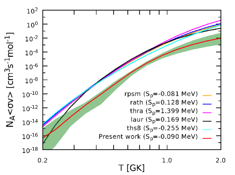
Figure 1.— Reaction rates of the ⁶⁴Ge($p$,$\gamma$)⁶⁵As reaction (in units of cm³ mol^-1 s^-1). The Present rate (red line) together with the upper and lower limits deduced from uncertainties are shown by a (green) colored band. Other available rates from JINA REACLIB (Cyburt et al., 2010) are shown for comparison. See details in the text and Table 4. (A color version of this figure is available in the online journal.)

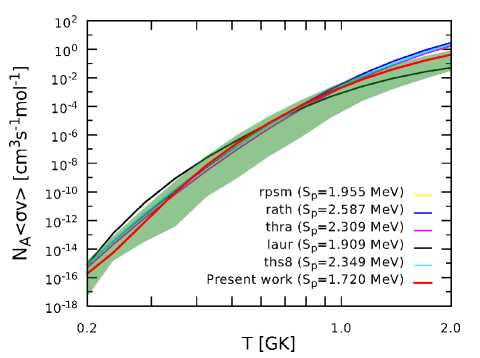
Figure 2.— As Fig. 1, but for the ⁶⁵As($p$,$\gamma$)⁶⁶Se reaction. Note the rpsm rate is quite close to the rath, ths8 and thra rates at different temperature regions (Cyburt et al., 2010), and hence the corresponding line is not clearly visible. See details in the text and Table 4. (A color version of this figure is available in the online journal.)

Figure 1 shows the comparison of the Present ⁶⁴Ge($p$,$\gamma$)⁶⁵As rate with others compiled in JINA REACLIB: rpsm, rath, thra, laur, and ths8. Note that only the rpsm rate uses an $S_{p}$(⁶⁵As) value that is within 1$\sigma$ of the recently determined experimental value. The Present rate differs significantly from others in the temperature region of interest in XRBs. The disagreement, in particular with the rpsm rate, demonstrates that the statistical-model is not applicable for this reaction owing to the low density of excited states in ⁶⁵As.

Similarly, the comparison of the Present ⁶⁵As($p$,$\gamma$)⁶⁶Se rate with other rates available in the JINA REACLIB: rpsm, rath, thra, laur, and ths8, is presented in Fig. 2. Only the laur and rpsm rates use $S_{p}$(⁶⁶Se) values that are within 1$\sigma$ of the currently accepted value. Although the Present rate differs significantly from the others, especially at lower and higher temperature regions, it is consistent with all others within the remaining large uncertainties. At $T>$1 GK, the laur rate is the lowest rate simply because only three excited states were considered by Van Wormer et al. (1994). It should be noted that the shell model calculation provides the first reliable estimate of the uncertainty of the ⁶⁵As($p$,$\gamma$) reaction rate, especially as the Hauser-Feshbach rates may suffer from unknown systematic errors due to the limited applicability of the statistical model near the proton drip line.

Uncertainties for the Present ⁶⁴Ge($p$,$\gamma$)⁶⁵As and ⁶⁵As($p$,$\gamma$)⁶⁶Se rates were estimated by considering the uncertainties in the $S_{p}$ values ($\pm$85 keV for ⁶⁵As and $\pm$310 keV for ⁶⁶Se) and estimated uncertainties in the calculated level energies ($\pm$168 keV for both ⁶⁵As and ⁶⁶Se (Honma et al., 2002)). These were added in quadrature to give uncertainties of $\pm$188 keV and $\pm$353 keV for the resonance energies $E_{r}$ of ⁶⁴Ge($p$,$\gamma$)⁶⁵As and ⁶⁵As($p$,$\gamma$)⁶⁶Se, respectively. Note that for the two known levels, i.e., $E_{x}$=187 keV in ⁶⁵As and $E_{x}$=2064 keV in ⁶⁶Se, an experimental excitation energy uncertainty of $\pm$3 keV is used instead. For ⁶⁴Ge($p$,$\gamma$)⁶⁵As, all resonance strengths $\omega\gamma$ are proportional to $\Gamma_{p}$ since $\Gamma_{p}$$\ll$$\Gamma_{\gamma}$ (see Table 1 and Eq. 3). The uncertainties in $\Gamma_{p}$ (or $\omega\gamma$) owing to the uncertainties in $E_{r}$ are calculated based on the energy dependence expressed in Eq. 5. In the case of ⁶⁵As($p$,$\gamma$)⁶⁶Se, only five resonances (at $E_{r}$=0.333, 0.557, 0.754, 0.836 and 1.061 MeV dominate the resonant rate within the temperature region of 0.2–2 GK. Here, the resonant strengths $\omega\gamma$ are proportional to $\Gamma_{p}$ for the first four resonances, while the strength of the last resonance at 1.061 MeV (dominating over $\sim$0.9–2 GK) depends on both, $\Gamma_{p}$ and $\Gamma_{\gamma}$. Uncertainties in $\Gamma_{\gamma}$ can be neglected because of the much larger rate uncertainties caused by $E_{r}$ and $\Gamma_{p}$. The uncertainties for all resonances listed in Table 2 are considered in the present calculations.

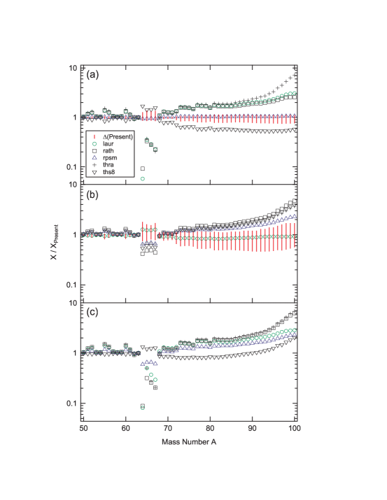
Figure 3.— Final abundances, as mass fractions $X$, following one-zone XRB calculations using the K04 thermodynamic history (Parikh et al., 2008, 2009). Results using rates determined in the Present work and in JINA REACLIB: rpsm, rath, thra, laur, and ths8 are indicated. Panels (a) and (b) show the effects of using either different ⁶⁴Ge($p$,$\gamma$) or different ⁶⁵As($p$,$\gamma$) rates, respectively, while panel (c) shows the effect of using different ⁶⁴Ge($p$,$\gamma$) and ⁶⁵As($p$,$\gamma$) rates together. The impact of the uncertainties in the Present ⁶⁴Ge($p$,$\gamma$) and ⁶⁵As($p$,$\gamma$) rates (see Figs. 1 and 2) is indicated as $\Delta$(Present) in panels (a) and (b). (A color version of this figure is available in the online journal.)

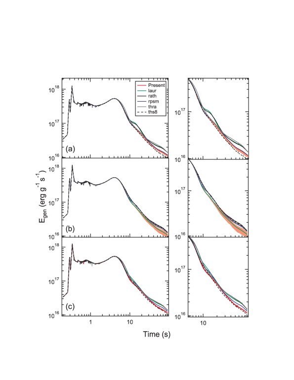
Figure 4.— As Fig. 3, but for nuclear energy generation rates $E_{\mathrm{gen}}$ during the burst in the K04 XRB model. Panels (a) and (b) show the effects of using either different ⁶⁴Ge($p$,$\gamma$) or different ⁶⁵As($p$,$\gamma$) rates, respectively, while panel (c) shows the effect of using different ⁶⁴Ge($p$,$\gamma$) and ⁶⁵As($p$,$\gamma$) rates together. The impact of the uncertainties in the Present ⁶⁴Ge($p$,$\gamma$) and ⁶⁵As($p$,$\gamma$) rates (see Figs. 1 and 2) is indicated in panels (a) and (b). Panels to the right show expanded views of the panels to the left. (A color version of this figure is available in the online journal.)

4. Astrophysical implication

We examine the impact of our new ⁶⁴Ge($p$,$\gamma$) and ⁶⁵As($p$,$\gamma$) rates and their uncertainties on the $rp$-process using one-zone XRB models. Post processing calculations using temperature and density trajectories from the literature enable a quick assessment of the impact of nuclear physics changes on the strength of the ⁶⁴Ge waiting point using the $A=64$ abundance, and on the burst energy generation rate. We use the post-processing approach for the K04 X-ray burst model (Parikh et al., 2008, 2009). However, postprocessing calculations do not take into account the changes in temperature and density that result from the energy generation changes. They can therefore not predict reliably the quantitative impact on produced abundances and light curves. To account for this effect, we also use the full one-zone X-ray burst model (Schatz et al., 2001), which represents a more extreme burst with very hydrogen rich ignition.

4.1. Post processing results for K04

With the representative K04 thermodynamic history (Parikh et al., 2008, 2009), final abundances (as mass fractions $X$) and the nuclear energy generation rate $E_{\mathrm{gen}}$ during a burst have been studied by performing separate XRB model calculations with different rates. In the K04 model, the peak temperature $T_{\mathrm{peak}}=1.4$ GK is similar to those reached at the base of the envelope in comparable hydrodynamic XRB models (e.g., 1.3 GK in José et al. (2010)). Figs. 3 and 4 compare results for $X$ and $E_{\mathrm{gen}}$ using rates from the present work to results using rates available in JINA REACLIB: laur, rath, rpsm, thra, ths8. The impact of (a) using different ⁶⁴Ge($p$,$\gamma$) rates (with the ⁶⁵As($p$,$\gamma$) rate held constant at the Present value), (b) using different ⁶⁵As($p$,$\gamma$) rates (with the ⁶⁴Ge($p$,$\gamma$) rate held constant at the Present value) and (c) using different ⁶⁴Ge($p$,$\gamma$) and ⁶⁵As($p$,$\gamma$) rates together, is indicated in each of the two figures. For each change in reaction rate, the corresponding inverse reaction rate is also changed to maintain detailed balance. This inverse rate strongly depends on the adopted reaction $S_{p}$ -value for the respective forward rate. As we compare the impact of different rates that have been determined using very different $S_{p}$ values (see Sect. 2 and Figs. 1 and 2), the results illustrate not only the influence of the rate calculation, but also the influence of different forward to reverse rate ratios due to different $S_{p}$-values.

The results of Figs. 3 and 4 are interesting, but not entirely unexpected. For the case of the ⁶⁴Ge($p$,$\gamma$) reaction, an equilibrium between the rates of the forward ($p$,$\gamma$) and reverse ($\gamma$,$p$) processes is quickly established due to the small ($p$,$\gamma$) $Q$-value relative to $kT$ at XRB temperatures: at 1 GK, $kT\approx 100$ keV. As a result, it is the ($p$,$\gamma$) $Q$-value, rather than the actual ⁶⁴Ge($p$,$\gamma$) rate, that is the most important nuclear physics quantity needed to characterize the equilibrium abundance of ⁶⁵As (and the subsequent flow of material to heavier nuclei through the ⁶⁵As($p$,$\gamma$) reaction), c.f. Schatz et al. (1998); Iliadis (2007); Parikh et al. (2009). This is nicely illustrated in Fig. 3(a): the ⁶⁴Ge($p$,$\gamma$) rates adopting positive ($p$,$\gamma$) $Q$-values (thra, laur, rath) give relatively lower final abundances around $A=64$ and larger abundances at higher masses precisely because of the larger equilibrium abundances of ⁶⁵As during the burst, allowing for increased flows of abundances to higher masses via the ⁶⁵As($p$,$\gamma$) reaction. On the other hand, the opposite is true for those rates adopting negative ($p$,$\gamma$) $Q$-values (ths8, Present, rpsm) because of the larger equilibrium abundances of ⁶⁴Ge and lower relative abundances of ⁶⁵As during the burst. Indeed, the summed mass fractions of species with $A>70$, $X_{70}$, vary considerably for different choices of $Q$-values. For example, when the thra, ths8 or Present rates are adopted, $X_{70}$ = 0.58, 0.21, or 0.33, respectively.

A consequence of the increased flow of abundances to heavier nuclei is seen in Fig. 4(a), where the models adopting the thra, laur, and rath rates give the largest $E_{\mathrm{gen}}$ at late times due to energy released from the decay of the larger amounts of heavy nuclei produced during the burst. As expected, the opposite is true for $E_{\mathrm{gen}}$ in the models using the ths8, Present and rpsm rates. We note that the predictions for $E_{\mathrm{gen}}$ at late times vary rather significantly between the models using the different rates, with differences as large as a factor of $\approx$ 2.

For the case of the ⁶⁵As($p$,$\gamma$) reaction, where a large positive ($p$,$\gamma$) $Q$-value is adopted in all rate estimates, the importance of the actual rate is illustrated in Fig. 3(b). The model adopting the largest rate at the most relevant temperatures ($T>0.9$ GK, c.f. José et al. (2010)), rath, gives the lowest abundances around $A=64$ and the largest abundances at higher masses. Again, as expected, the opposite is true for the model using the lowest ⁶⁵As($p$,$\gamma$) rate, laur. The variation in $X_{70}$ for different choices of the ⁶⁵As($p$,$\gamma$) rate is significant, with $X_{70}$ = 0.49 with the rath rate, and 0.29 with the laur rate. The behavior of $E_{\mathrm{gen}}$ for these models is again in accord with the distributions of the final abundances, with the largest $E_{\mathrm{gen}}$ at late times arising from the model using the rath rate, and the lowest $E_{\mathrm{gen}}$ arising from the model using the laur rate.

Finally, the effects of using different ⁶⁴Ge($p$,$\gamma$) and ⁶⁵As($p$,$\gamma$) rates from the same theoretical model calculation are shown in Figs. 3(c) and 4(c). This reveals the impact of competing influences from these two rates. For example, the model using the ths8 ⁶⁴Ge($p$,$\gamma$) rate gave the lowest relative abundances at higher masses (see Fig. 3(a)), while the model using the ths8 ⁶⁵As($p$,$\gamma$) rate gave among the highest relative abundances at higher masses (see Fig. 3(b)). When these two rates are used together, the combined impact on the final abundances (and $E_{\mathrm{gen}}$) is, not surprisingly, moderated.

Fig. 3(c) also shows that using the Present ⁶⁴Ge($p$,$\gamma$) and ⁶⁵As($p$,$\gamma$) rates results in the strongest ⁶⁴Ge waiting point, and the lowest final abundances at the highest masses. Differences with respect to predictions using rates from JINA REACLIB are as large as a factor of $\approx$ 7 at individual values of $A$. $X_{70}$ calculated with the two Present rates differs by as much as factor of 1.8 from models using the other rates.

We have also examined the impact on XRB model predictions of our uncertainties in the Present ⁶⁴Ge($p$,$\gamma$) and ⁶⁵As($p$,$\gamma$) rates, as shown in Figs. 1 and 2. Reverse rates for the lower and upper forward rates were determined using exactly the $Q$-values adopted for the corresponding forward rate calculations. Panels (a) and (b) of Figs. 3 and 4 show how these rate uncertainties affect final abundances and $E_{\mathrm{gen}}$ in the K04 model, with mass fractions above $A=64$ varying by up to a factor of 3 due to the individual uncertainties in the rates, $X_{70}$ varying by up to a factor of 2, and $E_{\mathrm{gen}}$ varying by up to 35% at late times. The impact on $X$ and $E_{\mathrm{gen}}$ of the uncertainties in the Present rates is somewhat smaller than that from different choices of rates but clearly not insignificant. As such, the mass of ⁶⁶Se should be determined experimentally and the uncertainty in the mass of ⁶⁵As should be reduced to better constrain model predictions.

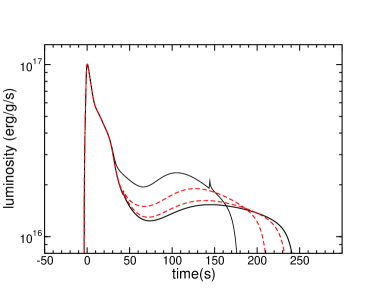
Figure 5.— Luminosity per gram of material calculated with the one-zone X-ray burst model for nuclear physics input that, within uncertainties, maximally favours (initially high solid line) and maximally disfavours (initially low solid line) the $rp$-process flow through the ⁶⁴Ge waiting point. The dashed lines show the results when only the ⁶⁵As($p$,$\gamma$) reaction rate is changed within uncertainties, and all other nuclear physics input is fixed. (A color version of this figure is available in the online journal.)

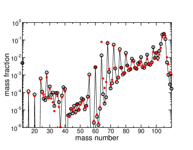
Figure 6.— Final mass fractions, summed by mass number, calculated with the one-zone X-ray burst model for nuclear physics input that, within uncertainties, maximally favours (open black circles, solid line) and maximally disfavours (filled red circles) the $rp$-process flow through the ⁶⁴Ge waiting point. (A color version of this figure is available in the online journal.)

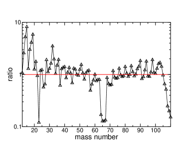
Figure 7.— Ratio of the final mass fractions shown in Fig. 6.

4.2. One-zone X-ray burst model results

In addition we explored the impact of the remaining nuclear physics uncertainties related to the ⁶⁴Ge waiting point on the full one-zone X-ray burst model described in Schatz et al. (2001). We note that this model is different from K04. It represents a burst that ignites in a very hydrogen rich environment, for example at high accretion rates and very low accreted metallicity, and was developed to explore the maximum extent of the $rp$-process towards heavy elements. To determine the total remaining uncertainty in the burst model due to the nuclear physics of the ⁶⁴Ge waiting point, we performed two extreme calculations. The calculations assume the most favourable (unfavourable) nuclear physics choice for the $rp$-process to pass through the ⁶⁴Ge waiting point, adopting the upper (lower) limit of the ⁶⁴Ge($p$,$\gamma$) and ⁶⁵As($p$,$\gamma$) reaction rates, and the upper (lower) limits of $S_{\rm p}(^{65}$As) and $S_{\rm p}(^{66}$Se). Varying $S_{\rm p}$ values independently, rather than varying individual masses, is justified as the uncertainties in $S_{\rm p}(^{65}$As) and $S_{\rm p}(^{66}$Se) are each completely dominated by the mass uncertainty of ⁶⁵As and ⁶⁶Se, respectively. Figs. 5 and 6 show the impact of the nuclear physics uncertainties on burst light curve and final composition. Clearly the nuclear physics uncertainties have a strong impact on observables. The abundance ratio of $A=64$ to $A=68$, a measure for the strength of the ⁶⁴Ge waiting point varies from 1.1 (making ⁶⁴Ge the strongest waiting point) to 0.2 (making ⁶⁴Ge not a significant waiting point). This is consistent with the result from Tu et al. (2011) who found that with their new ⁶⁵As mass ⁶⁴Ge is only a weak waiting point. However, as we show here, when taking into account all nuclear physics uncertainties, a strong ⁶⁴Ge waiting point cannot be ruled out. Fig. 7 shows the ratio of the final abundances. Similar to the results obtained for model K04 using post-processing, a weak ⁶⁴Ge waiting point (low ⁶⁴Ge abundance) leads to an enhancement of the production of heavier elements by up to a factor of 2. As already noted by Tu et al. (2011) the production of the heaviest nuclei with $A\geq 106$ is however reduced for a weak ⁶⁴Ge waiting point. This somewhat counter intuitive result is a consequence of the faster burning at higher temperature, which leads to a shorter burst as hydrogen is consumed more quickly. This effect is not seen in the post-processing calculation because there the temperature trajectory is fixed.

We also investigated the relative contributions of the various nuclear physics uncertainties. Similar to the K04 post processing results we find that the ⁶⁴Ge($p$,$\gamma$) reaction rate itself, for a fixed $Q$-value, has no influence on the burst model due to ($p$,$\gamma$)-($\gamma$,$p$) equilibrium between ⁶⁴Ge and ⁶⁵As. A calculation where only $S_{\rm p}(^{65}$As) and $S_{\rm p}(^{66}$Se) changes produced virtually the same result as the full variation, demonstrating that the mass uncertainties currently dominate. Changing each $S_{\rm p}$ separately indicates that the 85 keV uncertainty of $S_{\rm p}(^{65}$As) due to the ⁶⁵As mass uncertainty, and the 310 keV uncertainty of $S_{\rm p}(^{66}$Se) mainly due to the unknown ⁶⁶Se mass contribute roughly equally. However, varying the ⁶⁵As($p$,$\gamma$) reaction rate within our new uncertainties, while leaving $S_{\rm p}(^{65}$As) and $S_{\rm p}(^{66}$Se) fixed at their nominal values, still led to significant light curve changes (see Fig. 5) and a change of the $A=64$ to $A=68$ ratio from 1 to 0.7. This shows that once the mass uncertainties are addressed, the ⁶⁵As($p$,$\gamma$) reaction rate uncertainty will still play a role (even though fixing $S_{\rm p}(^{66}$Se) will reduce the rate uncertainty somewhat).

5. Summary and conclusion

We have determined new thermonuclear rates for the ⁶⁴Ge($p$,$\gamma$)⁶⁵As and ⁶⁵As($p$,$\gamma$)⁶⁶Se reactions based on large-scale shell model calculations and proton separation energies for ⁶⁵As and ⁶⁶Se derived using measured masses and, for ⁶⁶Se, the AME2012 extrapolation. These rates differ strongly from other rates available in the literature. For example, at $\approx$ 1 GK, our ⁶⁴Ge($p$,$\gamma$) rate is up to a factor of $\approx$ 90 lower than other rates, while our ⁶⁵As($p$,$\gamma$) rate differs by up to a factor of $\approx$ 3 from other rates.

We also determined for the first time reliable uncertainties for the ⁶⁴Ge($p$,$\gamma$)⁶⁵As and ⁶⁵As($p$,$\gamma$)⁶⁶Se reactions. We find that in two different X-ray burst models, the remaining uncertainties in $S_{\rm p}(^{65}$As), $S_{\rm p}(^{66}$Se), and the ⁶⁵As($p$,$\gamma$) reaction rate lead to large uncertainties in the strength of the ⁶⁴Ge waiting point in the $rp$-process, the produced amount of $A=64$ material in the burst ashes that will ultimately decay to ⁶⁴Zn, the produced amount of heavier nuclei beyond $A=64$, and the burst light curve. These effects are robust and appear in two different X-ray burst models. We conclude that to address these uncertainties a more precise measurement of the ⁶⁵As mass, a measurement of the ⁶⁶Se mass, and a measurement of the excitation energies of states in ⁶⁶Se that serve as important resonances for the ⁶⁵As($p$,$\gamma$)⁶⁶Se reaction will be important.

References

- Angulo et al. (1999) Angulo, C., et al., 1999, Nucl. Phys. A, 656, 3
- Audi & Wapstra (1995) Audi, G. & Wapstra, A.H. 1995, Nucl. Phys. A595, 409
- Audi et al. (2003) Audi, G., et al., 2003, Nucl. Phys. A, 729, 337
- Audi et al. (2012) Audi, G., et al., 2012, Chin. Phys. C, 36, 1157
- Bertulani et al. (2003) Bertulani, C.A., et al., 2003, Comput. Phys. Commun. 156, 123
- Brown et al. (2002) Brown, B.A., et al., 2002, Phys. Rev. C, 65, 045802
- Brown & Rae (2014) Brown, B.A. & Rae, W.D.M. 2014, Nucl. Data Sheets 120, 115
- Brown (2014) Brown, B. A., (WSPOT code), http://www.nscl.msu.edu/brown/reaction-codes/home.html
- Browne & Tuli (2010) Browne, E. & Tuli, J.K. 2010, Nucl. Data Sheets 111, 2425
- Brussaard & Glaudemans (1977) Brussaard, P.J. & Glaudemans, P.W.M. 1977, Shell model Applications in Nuclear Spectroscopy (North-Holland, Amsterdam)
- Clark et al. (2007) Clark, J.A., et al., 2007, Phys. Rev. C, 75, 032801
- Cyburt et al. (2010) Cyburt, R.H., et al., 2010, ApJS, 189, 240
- Elomaa et al. (2009) Elomaa, V.-V., et al., 2009, Phys. Rev. Lett., 102, 252501
- Fisker et al. (2008) Fisker, J.L., et al., 2008, ApJS, 174, 261
- Fowler et al. (1964) Fowler, W.A., et al., 1964, ApJS, 9, 201
- He et al. (2014) He, J.J., et al., 2014, Phys. Rev. C, 89, 035802
- Herndl et al. (1995) Herndl, H., et al., 1995, Phys. Rev. C, 52, 1078
- Honma et al. (2002) Honma, M., et al., 2002, Phys. Rev. C, 65, 061301R
- Honma et al. (2004) Honma, M., et al., 2004, Phys. Rev. C, 69, 034335
- Honma et al. (2005) Honma, M., et al., 2005, Eur. Phys. J. A 25(S01), 499
- Huang et al. (2010) Huang, J.T., et al., 2010, At. Data Nucl. Data Tables 96, 824
- Iliadis (2007) Iliadis, C. 2007, Nuclear Physics of Stars (Wiley, Weinheim)
- José et al. (2010) José, J., et al., 2010, ApJS, 189, 204
- Joss (1977) Joss, P.C. 1977, Nature 270, 310
- Lam et al. (2016) Lam, Y.H., et al., 2016, in preparation
- Lewin et al. (1993) Lewin, W., et al., 1993, Space Sci. Rev., 62, 223
- Möller et al. (1995) Möller, P., et al., 1995, At. Data Nucl. Data Tables 59, 185
- Obertelli et al. (2011) Obertelli, A., et al., 2011, Phys. Lett. B 701, 417
- Parikh et al. (2008) Parikh, A., et al., 2008, ApJS, 178, 110
- Parikh et al. (2009) Parikh, A., et al., 2009, Phys. Rev. C, 79, 045802
- Parikh et al. (2013) Parikh, A., et al., 2013, Prog. Part. Nucl. Phys., 69, 225
- Parikh et al. (2014) Parikh, A., José, J., Sala, G., 2014, AIP Advances 4, 041002
- Pearson et al. (1996) Pearson, J.M., et al., 1996, Phys. Lett. B 387, 455
- Rauscher & Thielemann (1998) Rauscher, T. & Thielemann, F.-K. 1998, in Stellar Evolution, Stellar Explosions and Galactic Chemical Evolution, edited by Mezzacappa, A. (IOP, Bristol)
- Rauscher & Thielemann (2000) Rauscher, T. & Thielemann, F.-K. 2000, At. Data Nucl. Data Tables 75, 1
- Richter et al. (2011) Richter, W. A. et al., 2011, Phys. Rev. C, 83, 065803
- Rolfs & Rodney (1988) Rolfs, C.E. & Rodney, W.S. 1988, Cauldrons in the Cosmos (Univ. of Chicago Press, Chicago)
- Ruotsalainen et al. (2013) Ruotsalainen, P., et al., 2013, Phys. Rev. C, 88, 041308
- Schatz (2006) Schatz, H. 2006, Int. J. Mass Spectrom., 251, 293
- Schatz et al. (1998) Schatz, H., et al., 1998, Phys. Rep., 294, 167
- Schatz et al. (2001) Schatz, H., et al., 2001, Phys. Rev. Lett., 86, 3471
- Schatz et al. (2005) Schatz, H., et al., 2005, Phys. Rev. C, 72, 065804
- Schatz & Rehm (2006) Schatz, H. & Rehm, K.E. Nucl. Phys. A, 777, 601
- Schury et al. (2007) Schury, P., et al., 2007, Phys. Rev. C, 75, 055801
- Strohmayer & Bildsten (2006) Strohmayer, T.E. & Bildsten, L. 2006, in: Lewin, W. & van der Klis, M. (Eds.), Compact Stellar X-Ray Sources (Cambridge Univ. Press, Cambridge)
- Tu et al. (2011) Tu, X. L., et al., 2011, Phys. Rev. Lett., 106, 112501
- Van Wormer et al. (1994) Van Wormer, L., et al., 1994, ApJ, 432, 326
- Wallace & Woosley (1981) Wallace, R.K. & Woosley, S.E. 1981, ApJS, 45, 389
- Wang et al. (2012) Wang, M., et al., 2012, Chin. Phys. C, 80, 1603
- Woosley & Taam (1976) Woosley, S.E. & Taam, R.E. 1976, Nature 263, 101
- Woosley et al. (2004) Woosley, S.E., et al., 2004, ApJS, 151, 75
- Xia et al. (2002) Xia, J.W., et al., 2002, Nucl. Instr. Meth. A, 488, 11