On the Binary Frequency of the Lowest Mass Members of the Pleiades with Hubble Space Telescope Wide Field Camera 3

Abstract

We present the results of a Hubble Space Telescope Wide Field Camera 3 imaging survey of $11$ of the lowest mass brown dwarfs in the Pleiades known ($25-40$ $\mbox{M}_{\mbox{\tiny Jup}}$). These objects represent the predecessors to T dwarfs in the field. Using a semi-empirical binary PSF-fitting technique, we are able to probe to $0\farcs 03$ (0.75 pixel), better than 2x the WFC3/UVIS diffraction limit. We did not find any companions to our targets. From extensive testing of our PSF-fitting method on simulated binaries, we compute detection limits which rule out companions to our targets with mass ratios of $q\gtrsim 0.7$ and separations $a\gtrsim 4$ AU. Thus, our survey is the first to attain the high angular resolution needed to resolve brown dwarf binaries in the Pleiades at separations that are most common in the field population. We constrain the binary frequency over this range of separation and mass ratio of $25-40$ $\mbox{M}_{\mbox{\tiny Jup}}$ Pleiades brown dwarfs to be $<$$11\%$ for $1\sigma$ ($<$$26\%$ at $2\sigma$). This binary frequency is consistent with both younger and older brown dwarfs in this mass range.

1 Introduction

Hundreds of brown dwarfs have now been identified in the solar neighborhood through wide-field surveys (e.g. DENIS, 2MASS, SDSS, UKIDSS, Pan-STARRS and WISE) and in nearby star-forming regions (e.g., Epchtein et al. 1997; Delfosse et al. 1997; Chiu et al. 2006; Allers et al. 2006; Bihain et al. 2006; Reid et al. 2008; Bihain et al. 2010; Burningham et al. 2010; Cushing et al. 2011; Liu et al. 2011; Lodieu et al. 2012; Burningham et al. 2013). The study of brown dwarf binarity is a fundamental tool for testing theory, given that the statistical properties of binaries probe formation scenarios in the very low-mass regime (e.g., Burgasser et al. 2007; Bate 2009; Luhman 2012; Bate 2012). For the past decade, HST and ground-based adaptive optics (AO) have fueled such studies by searching for binaries among field ($0.5-5.0$ Gyr) brown dwarfs, (e.g., Martín et al. 1998; Burgasser et al. 2003; Bouy et al. 2003; Burgasser et al. 2006; Liu et al. 2006) and in young ($1-10$ Myr) star-forming regions such as Upper Sco (Kraus et al. 2005; Bouy et al. 2006b; Biller et al. 2011; Kraus & Hillenbrand 2012), Taurus (e.g. Kraus et al. 2006; Konopacky et al. 2007; Todorov et al. 2010; Kraus & Hillenbrand 2012; Todorov et al. 2014), and Chamaeleon I (e.g. Neuhäuser et al. 2002; Luhman 2004; Lafrenière et al. 2008; Ahmic et al. 2007; Luhman 2007). Multiplicity studies have also been performed in older ($\approx$$400$ Myr) regions such as Coma Ber, Praesepe, and the Hyades (Kraus & Hillenbrand 2007; Duchêne et al. 2013).

Previous work has shown that the binary frequency decreases and typical mass ratios increase going to lower mass primaries (Burgasser et al. 2007). One surprising finding is that these properties apparently differ between young and old binaries, with the binary frequency enhanced at young ages by a factor of $\approx$2$\times$ (e.g., Lafrenière et al. 2008) and with wide separations ($\approx$$10-1000$ AU) being much more common as compared to field brown dwarf binaries that are rarely wider than 10 AU (e.g. Burgasser et al. 2006; Close et al. 2007). An unambiguous physical explanation for this difference is lacking, as even relatively wide binaries in young star-forming regions (Luhman 2004; Luhman et al. 2009) are not expected to incur dynamical interactions of sufficient intensity to reduce their frequency and truncate their separation distribution.

The Pleiades open cluster serves as an important bridge between the youngest ($1-10$  Myr) brown dwarfs and the field population. It has several advantages, such as its well established age of $\approx$$125$ Myr (Stauffer et al. 1998; Barrado y Navascués et al. 2004) and distance of 136.2$\pm 1.2$ pc (Melis et al. 2014). There are many surveys that have searched for brown dwarf binaries in the Pleiades (Martín et al. 2000; Dobbie et al. 2002; Jameson et al. 2002; Nagashima et al. 2003; Moraux et al. 2003; Bouy et al. 2006a). However, there are only 4 Pleiades brown dwarfs with primary masses $\lesssim$40 $\mbox{M}_{\mbox{\tiny Jup}}$ that have been searched for companions to date (Moraux et al. 2003; Bouy et al. 2006a). At such masses, these objects will cool to T dwarfs at ages of the field population.

In this work, we triple the number of low mass Pleiades brown dwarfs searched for companions, surveying a sample of 11 previously unobserved L dwarfs in the Pleiades using HST/WFC3. We computed detection limits for our sample using a binary fitting technique and Tiny Tim PSF models. We compared our binary frequency to the observed frequencies for brown dwarfs at similar masses in Taurus, Chamaeleon I, Upper Scorpius, and the field population.

2 Observations

2.1 Sample

We obtained images of 11 Pleiades brown dwarfs using the Hubble Space Telescope (HST) with the UVIS channel of Wide Field Camera 3 (WFC3/UVIS) in January and February of 2012 (GO 12563, PI Dupuy). Our sample consists of the faintest ($K\gtrsim 16$ mag), latest type ($\gtrsim$M9) members of the Pleiades known in early 2011. According to BT-Settl models of Allard (2014) tied to the COND evolutionary models of Baraffe et al. (1997, 1998, 2003), the estimated masses of our sample are $25-40$ $\mbox{M}_{\mbox{\tiny Jup}}$ based on their $K-$band magnitudes and the age of the Pleiades. When defining our sample, we considered objects bona-fide members of the Pleiades if they had proper motion indicating cluster membership and spectra with low surface gravity features or lithium absorption. Our sample is listed in Table 1, along with 4 targets from previous HST/ACS and HST/WFPC2 observations of Pleiades brown dwarfs by Martín et al. (2003) and Bouy et al. (2006a) that match our membership criteria. All of our sample have proper motions consistent with the Pleiades cluster (Bihain et al. 2006; Casewell et al. 2007; Lodieu et al. 2012). BRB 17, BRB 21, PLIZ 35, BRB 23 and BRB 29 have spectral types L0-L4.5 from Bihain et al. (2010).

2.2 HST/WFC3 Imaging

We obtained 2 exposures each in filters F814W and F850LP for each target star. One image of brown dwarf BRB 17 was lost due to a pointing error so we had a total of 43 images. The target stars are positioned near the center of the full field of view at $\approx$$250$ pixels from the bottom of chip 1. We chose a longer exposure time of 900 s in F814W filter, where we are sensitive to tighter brown dwarf binaries because of the smaller PSF. We also obtained 340 s exposures in F850LP to confirm the presence of any candidate companions and measure their colors. The full width half maximum of the PSF is $\approx$$1.84$ pixels in F814W and $\approx$$1.96$ pixels in F850LP according to the WFC3 data handbook.

We inspected each image for cosmic rays hits, identified as rays or streaks with high counts but not resembling WFC3 point sources. We found 6 of the 43 images had cosmic ray hits within 5 pixels of the target star. We use the Laplacian Cosmic Ray Identification algorithm LACOSMIC (van Dokkum 2001) to remove cosmic rays from a 200$\times$200 pixel area on the detector centered on the target star. LACOSMIC replaces each pixel with the median of the surrounding pixels in an iterative procedure. Visual inspection after the fact confirms that we successfully cleared all obvious cosmic ray hits except for a single image of brown dwarf BRB 23 in F850LP due to a cosmic ray hit through the center of the peak of the target. We excluded this image of BRB 23 in the subsequent data analysis, therefore leaving us with 42 images total for the rest of our analysis.

We computed aperture photometry of our targets from the pipeline calibrated, geometrically-corrected, dither-combined (drz) images. We calculated our aperture photometry using the APER task from the IDL Astronomy User’s Library for an aperture radius of $0\farcs 4$ and a sky annulus of $0\farcs 4-0\farcs 8$. We converted the flux in our aperture to a Vega magnitude using zeropoints of $24.57$ mag for the F814W filter and $23.20$ mag for the F850LP filter provided in the HST/WFC3 webpages. To determine our photometric uncertainties, we first constructed an error image for each image, accounting for read noise and poisson noise. Using a Monte Carlo approach, we determined our photometric errors from $10^{4}$ iterations of the APER task after adding random Gaussian noise to the image in each iteration. The resulting F814W and F850LP photometry for our targets is listed in Table 2.

3 Image Analysis

3.1 Point Spread Function (PSF) Model of WFC3/UVIS

In order to search for close companions to our targets, we began by fitting a model Tiny Tim (Krist et al. 2011) point spread function to our imaging data. To create the most accurate model we specified the exact coordinates of our target and used an input spectrum of 2MASS J00361617+1821104 (Reid et al. 2000, L3.5). We set the defocus parameter in Tiny Tim to the model defocus provided on the Space Telescope Science Institute webpage for each image of each target. The model defocus is computed to account for breathing, according to the telescope temperature data.

We sampled the Tiny Tim PSF at 5$\times$ the pixel scale ($0\farcs 04$ pixel^-1) of WFC3/UVIS1. To simulate sub-pixel shifts of our targets we bilinearly interpolated to an arbitrary fractional pixel and then binned down to pixel scale of WFC3. We used the Nelder-Mead downhill simplex method from Press (1988), which is the AMOEBA algorithm in IDL, to minimize the $\chi^{2}$, varying the $(x,y)$ position and flux normalization until finding the best fit. We computed $\chi^{2}$ as ((image-model)/noise)², where “noise” is the noise image provided by the WFC3 reduction pipeline. We ran the AMOEBA algorithm twice, starting the second run at the end point in parameter space of the first run, as recommended by Press (1988). We fit a $\pm 10$ pixel cutout region centered on the target star.

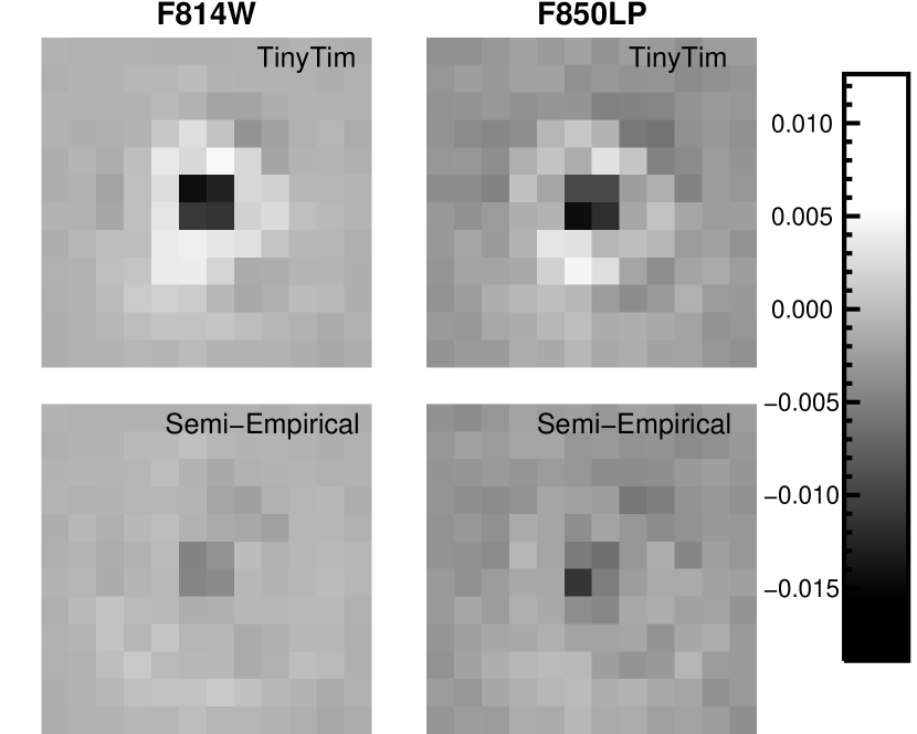
Figure 1: The average residuals of all WFC3 images after fitting the original Tiny Tim model (top) and fitting our semi-empirical PSF model (bottom). For viewing purposes, we display the average residuals as the normalized “(image-model)” in each filter. When using our original Tiny Tim model, the average residuals results in concentrated residual flux at instrumental position angles of $30-50^{\circ}$ and $150-170^{\circ}$ for both the F814W and F850LP filters. This would bias our binary fitting technique to preferentially recover companions with these position angles. Therefore we computed a semi-empirical model PSF using the original Tiny Tim model as a starting point as detailed in §3.1. The resulting average residuals are improved by a factor of 4-5$\times$ from $\approx 5\%$ and $\approx 6\%$ to $\approx 0.9\%$ and $\approx 2.3\%$ in F814W and F850LP respectively. The residuals are also smoother, no longer containing concentrations at position angles of $30-50^{\circ}$ and $150-170^{\circ}$.

We found average residuals after subtracting the best-fit Tiny Tim model of $5\%$ and $6\%$ for F814W and F850LP images, respectively. We computed residuals of our fits as the average fractional offset between the image and the model. The majority of the residual flux using the Tiny Tim model was at instrumental position angles of $30-50^{\circ}$ and $150-170^{\circ}$ in both the F814W and F850LP filters (Figure 1). If we searched for faint companions using the TinyTim PSF model and our binary fitting technique detailed below, we found that this systematic residual flux led to spurious detections of companions at these position angles.

Therefore, we instead computed a single optimal semi-empirical PSF model that minimized the residuals across all images by modifying the Tiny Tim model. We iteratively solved for a 5$\times$ over-sampled additional component image to be added to the Tiny Tim model. The best guess of this additional component at each pixel was computed as the median across all normalized images of the data minus the previous iteration’s PSF model. We computed a semi-empirical PSF model as the Tiny Tim model at the mean position of our targets with this additional component added in.

Using our semi-empirical PSF model, the final residuals of our fits were improved by 5$\times$ to $\approx$$0.9\%$ and $\approx$$2.3\%$ for F814W and F850LP, respectively (Figure 1). Most importantly, we no longer see the concentrated residual flux at position angles of $150-170^{\circ}$. We use our semi-empirical PSF model in all subsequent analysis.

The method of fitting binaries is the same as described above, but instead of using a single model we use two co-added models. As before, the AMOEBA algorithm minimizes the $\chi^{2}$ between the image and co-added semi-empirical PSFs. We varied six binary parameters: the primary’s position on detector, the flux normalization between the primary star and the PSF model primary, the binary separation, the position angle, and flux ratio between the primary and secondary.

3.2 Quantifying False Positives

If we run our binary fitting code on a image of a single star, we recover binary parameters of false positive companions. By definition, these detections reveal the distribution in separation and flux ratio of the false positives we would find while searching for companions in our imaging data. To characterize the false positives for our WFC3 data, we fit images of our target stars using our binary fitting technique from §3.1. We scale all images to either the median or minimum S/N of our sample by adding in gaussian noise (Table 3). This allows us to put our sample on a common scale for our simulations. For each target star, we start with 150 random initial guesses, uniformly distributed in ($x,y$) from $0.1-5$ pixels, and flux ratios from $0-5$ mag.

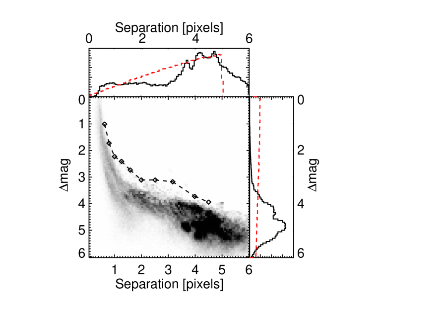
Figure 2: Number density of binary parameters returned when fitting images of single stars with a binary PSF model, i.e., false positive detections, for the median S/N F814W case. Overall, the most common false positives have wide with separations of $>$3 pixels, and faint flux ratios of $>$4 mag companions, but at separations of $<$1 pixels ($<$$0\farcs 04$), the majority of false positives range with flux ratios of $0-3$ mag. The dotted red histograms are the initial guesses for the false positives uniformly distributed in log separation and flux ratio. The 1% false positive curve (§3.4) is over plotted (diamonds).

We show the resulting distribution of separations vs flux ratios of recovered false positives in Figure 2. The brightness of false positives increases with decreasing separation. At the tightest separations ($<$$0\farcs 02$, $<$$0.6$ pixel), we find that near unity flux ratio false positives are the most common. At wider separations ($>$1.5 pixels, $>$$0\farcs 06$), we find that almost all false positives are found with large flux ratios of $3-5$ mag. This is expected, as the binary fitting code is required to return a position and flux normalization for a secondary even if one doesn’t exist. In other words, the single WFC3 PSF can be fit with a model of a high flux PSF and a very low flux PSF added in to fit any small leftover residuals.

3.3 Artificial Binary Simulations

In order to compute detection limits for our survey, we generated artificial binaries at random separations of $0.3-5$ pixels ($0\farcs 018-0\farcs 2$), position angles of $0-360^{\circ}$, and flux ratios of $0-5$ mag. We created these artificial binaries by shifting, scaling and co-adding randomly selected pairs of actual images together. Given that the marginally sampled WFC3 PSF (FWHM $\lesssim$2 pixels) hinders the accuracy of linear interpolation at sub-pixel shifts, we shift the secondary star relative to the primary star in integer pixel steps. We scaled the image of every primary to a common S/N by adding noise, thus degrading the image to lower S/N. We scaled the secondary to a S/N appropriate for the randomly chosen flux ratio of the artificial binary.

Given the integer pixel shifts, there are fixed separations and position angles allowed by the possible image pairings. These integer pixel shifts can result in non-integer artificial binary separations because the sub-pixel position for each image varies. Out of all possible pairings we selected a subset of $4800$ artificial binaries that are distributed uniformly in log separation, flux ratio, and position angle. We ran two sets of simulations for each filter, scaling primaries alternatively to the median S/N and the minimum S/N of our images (Table 3). Only half the images were used for the median S/N simulations, given that we only scaled images down in S/N, never up.

We then blindly fitted for the binary parameters of our artificial binaries using a double PSF model as described in §3.1, using 150 random initial guesses. The best-fit values for each parameter are calculated as the mean of the resulting 150 runs of our binary fitting code parameters where runs with outlier $\chi^{2}$ were excluded from the average.

3.4 Deriving False Positive Curves

The binary parameters recovered in our artificial binary simulations contain a mix of both detections and false positives. To assess the likelihood of a given binary fit being a detection, we compared our distribution of false positives from §3.2 and our fits to artificial binaries from §3.3 to measure our false positive curve, i.e the largest flux ratio before the recovered secondary star becomes indistinguishable from a false positive at a given separation.

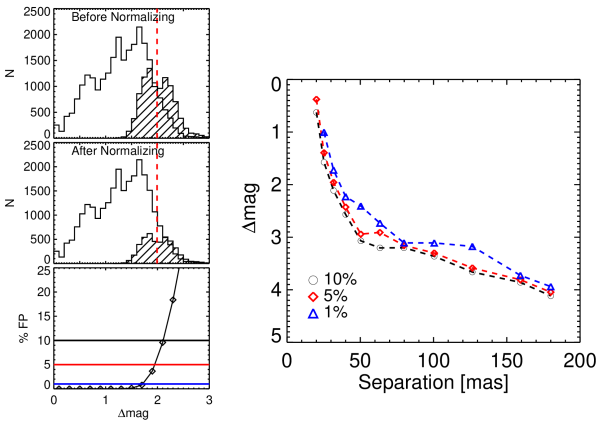
Figure 3: Illustration of our calculation of the false positive curve using the case of artificial binaries at separations $0.79-1.0$ pixels ($\approx 0\farcs 03-0\farcs 04$) as an example. TOP LEFT: The white histogram is the distribution of the recovered flux ratios $\Delta\rm m$ for artificial binaries at separations of $0.79-1.0$ pixels. The histogram with slashes are false positives recovered by using our binary fitting technique on single star images. The vertical red dashed line is the median false positive flux ratio. MIDDLE LEFT: We normalize the histogram of false positive flux ratios (slashes) to the white histogram of recovered artificial binary flux ratios by conservatively assuming that any artificial binaries with recovered flux ratios larger than the median false positive flux ratio (vertical dashed red line) are most likely false positives themselves. BOTTOM LEFT: 1% (black solid line), 5% (red) and 10% (blue) false positive fractions as a function of flux ratio. RIGHT: The false positive curve is constructed by repeating the process for all separation bins. The stars denote the $\Delta\rm m$ corresponding to $1\%,5\%$ and $10\%$ false positive fraction at separations of $0.79-1.0$ pixels shown at the bottom left.

We considered the artificial binaries and false positives in a given separation and flux ratio range, using 0.1 dex pixel bin widths and $0.3$ mag flux ratio bin widths, respectively. In each separation bin we normalized the histogram of false positive flux ratios to the histogram of recovered artificial binary flux ratios by conservatively assuming that any artificial binaries with recovered flux ratios larger than the median false positive flux ratio $\Delta\rm m_{\rm crit}$ were most likely false positives themselves. We computed this normalization factor as $\frac{n}{0.5n_{\rm fp}}$, where $n_{\rm fp}$ is the total number of false positives and $n$ is the number of artificial binaries with flux ratios $>$$\Delta\rm m_{\rm crit}$. After normalization, we computed the false positive fraction as a function of flux ratio as $1-\frac{n_{\rm fp}}{n}$. We repeat the procedure above for each separation bin. This procedure is depicted in Figure 3 for the $0.79-1.0$ pixel separation bin.

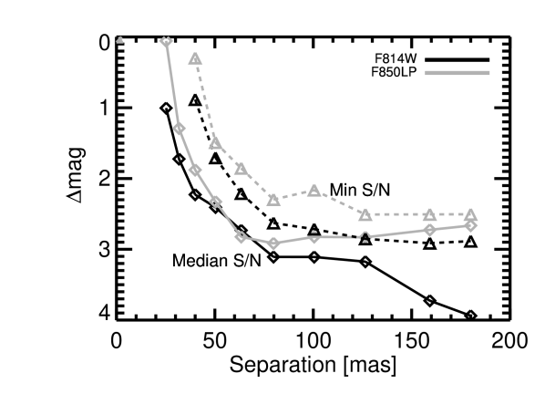
Figure 4: False positive curves computed at the minimum (triangles) and median (squares) signal-to-noise of our WFC3 images of Pleiades brown dwarfs (§3.4) for the F814W (black) and F850LP (grey) filters. As expected the minimum S/N false positive curves have brighter false positives than the median S/N curves in a given filter.

With the procedure detailed above, we computed false positive curves at the median and minimum S/N of our images for the F814W and F850LP filter as shown in Figure 4. Each of our false positive curves are representative of a single, S/N given that we scale our all our images to a common S/N for each set of simulations.

3.5 Deriving Contrast Curves

We computed contrast curves that correspond to the largest flux ratio companion that our binary PSF fitting technique can recover accurately at a given separation. A binary is considered “recovered” if the best fit parameters are within $0.2$ pixels and $1$ mag of the input $(x,y)$ positions and flux ratio, respectively. We binned our simulated binaries by separation and flux ratio with bin widths of 0.1 dex pixels and $0.3$ mag, respectively. In each bin, we computed the completeness fraction as the number of artificial binaries that are recovered divided by the total number of artificial binaries in the bin. We define our contrast curves as the flux ratio bin at a given separation where the completeness fraction is $90\%$ determined by the interpolation of the binned results. We computed contrast curves at the median and minimum S/N of our targets (Table 3) for the both F814W and F850LP filters.

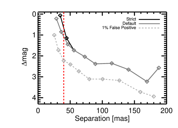
Figure 5: Contrast curves for the median F814W S/N case constructed using our default and a stricter companion recovery criteria (see §3.5). In our default criteria, we required companions be recovered to within $1$ mag of the input binary parameters (dark grey solid line). We can recover companions with flux ratios $<$1 mag and separations $>$$0\farcs 04$. We also tested a stricter criteria, and required recovered companions to be within within $0.3$ mag of the input flux ratio (black solid line). The contrast curves are identical for separations $>$$0\farcs 055$. With the stricter recovery criteria, companions with separations $<$$0\farcs 04$ and flux ratios $<0.5$ mag were detectable. Both contrast curves required that recovered artificial binaries be within $0.2$ pixels of input ($x,y$) position. We adopt our default criteria given that most brown dwarf binaries are found to have near unity flux ratios. The 1% false positive curve is shown for comparison (light grey dotted line). The contrast curve drops at 200 mas due to difficulty in fitting artificial binaries at the edge of our cut-out region of $\pm 10$ pixels.

Figure 5 shows our resulting contrast curves. We are able to recover tight ($<$$0\farcs 04$, $<$1 pixel) binaries with flux ratios $\lesssim$1 mag. At wider separations we recover binaries $3-5$ magnitudes fainter. We also constructed a contrast curve with a stricter recovery requirement to be within $0.3$ mag of the input. This leads to a contrast curve that reaches in to binary separations of $0\farcs 035$ (0.9 pixels) and is identical to our default recovery requirements outside $0\farcs 055$ (1.4 pixels). A flux ratio of $\lesssim$1 mag for our targets corresponds to a mass ratio $q\gtrsim 7$ which allows us to rule out the possibility of Pleiades brown dwarf binaries similar to field brown dwarf binaries, since the latter mostly have $q\approx 1$ (see review by Burgasser et al. 2007). This means that a stricter flux ratio requirement of $<$$0.3$ mag for constructing our contrast curves is unnecessary. Thus, our PSF fitting technique is able to recover artificial binaries as tight as $0\farcs 03$, well inside the diffraction limit ($\approx\frac{1}{3}\lambda/D$)

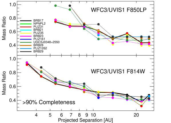
Figure 6: 90% completeness contrast curves for our F814W and F850LP observations of 11 young L dwarfs ($\lesssim$40$~{}\mbox{M}_{\mbox{\tiny Jup}}$) in the Pleiades. Our contrast curves rule out the majority of expected brown dwarf binaries, given that most binaries in the field have mass ratios $\gtrsim$$0.6$ and separations $<$25 AU (Burgasser et al. 2007). We convert our detection limit flux ratios in WFC3 bandpasses to mass ratios using the distance to the Pleiades ($136.2$ pc, Melis et al. 2014) and evolution models from Baraffe et al. (2003) tied to BT-Settl models (Allard 2014).

Given that each target in our sample has a different S/N, we interpolated over the measured median and minimum S/N curves to compute a contrast curve for each target. We conservatively fixed the contrast curve for our targets with S/N higher than the median S/N to the median S/N contrast curve. Our detection limits in F814W and F850LP mag for each target are shown in Table 4. These detection limits have lower contrast and are more conservative than the false positive curves, as expected. Finally, we convert our contrast curves from F814W and F850LP magnitudes to masses using BT-Settl models Allard (2014) tied to the COND evolution models of Baraffe et al. (2003). We assumed an age of $125$ Myr (Barrado y Navascués et al. 2004) and distance to the Pleiades of $136.2$  pc (Melis et al. 2014). Figure 6 shows the 90% completeness contrast curve for each target as a function of mass ratio ($q$) and projected separation ($a$) in AU. We use only the F814W contrast curve for our constraint on the binary frequency due to higher S/N, larger contrast, and closer limiting separation than our F850LP contrast curve.

3.6 Completeness Maps

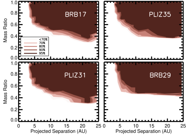
Figure 7: Example completeness maps for several our 11 young L dwarfs ($\lesssim$40$~{}\mbox{M}_{\mbox{\tiny Jup}}$) in the Pleiades. At each point, the completeness map represents the percentage of binaries that would have been recovered given our observations. We convert our detection limit flux ratios in WFC3 bandpasses to mass ratios using the distance to the Pleiades ($136.2$ pc, Melis et al. 2014), and evolution models from Baraffe et al. (2003) tied to BT-Settl models (Allard 2014).

Similar to how we derive contrast curves in §3.5, we derive a median and a minimum S/N completeness map for the F814W and F850LP filters. Each completeness map represents the probability that a companion with a given separation and flux ratio would have been detected (Figure 7). The procedure for deriving completeness maps is exactly as deriving a contrast curve in §3.5 except that we compute the completeness fraction at every separation and flux ratio bin. We computed a completeness map for each target similar to §3.5, by interpolating over the median and minimum S/N completeness maps. We conservatively fixed the completeness maps for our targets with S/N higher than the median S/N to the median S/N completeness map. Our completeness maps for several targets are shown in Figure 7.

4 Results

4.1 L Dwarf Binary Frequency of the Pleiades

We found no companions in surveying 11 brown dwarf members of the Pleiades with $K\gtrsim 16.0$ mag. Our F814W contrast curves demonstrate that we could have detected companions with mass ratios of $q\gtrsim 0.5$ at separations $a\gtrsim 10$ AU and $q\gtrsim 0.8$ at $a\gtrsim 4$ AU (Figure 6). Most known very low mass binaries are sharply peaked towards mass ratios $q\approx 1$ (Burgasser et al. 2006; Liu et al. 2010). Furthermore, our detection limits probe down to separations $a\approx 4$ AU, near the peak of the observed binary distribution (Burgasser et al. 2006). Thus, our detection limits are sensitive to the majority of binaries expected from the observed field population of T dwarfs (Burgasser et al. 2003, 2006; Gelino et al. 2011; Liu et al. 2012; Radigan et al. 2013).

We estimated the binary frequency for the Pleiades by comparing our completeness maps (§3.6) to various random simulated populations of binaries. Each population of binaries had an adopted eccentricity, mass ratio and separation distribution, with semi-major axes of $<$$25$ AU in accordance with observations of T dwarf binaries in the field. We adopted a uniform eccentricity distribution of $0-0.9$ in accordance with observations (Dupuy & Liu 2011). For our mass ratio distribution, we used the observed power law of $P(q)\propto q^{4.9}$ (Liu et al. 2010). For our separation distribution, we used the log normal distribution from Allen (2007). We assumed uniform prior distributions of longitude of ascending node, mean anomaly, and argument of periapsis, and an $a\sin{i}$ distribution for inclination. We projected each binary on sky from the population with $10^{5}$ randomly chosen orbits. We compared each of these $10^{5}$ orbits to each completeness map of each target. The probability for detecting a binary was given by our completeness fraction at the separation and mass ratio of the binary from the completeness maps (Figure 7). We averaged over all probabilities and computed a single average probability (“detectability”) to recover a companion for each target star (Table 6). Similar to Aberasturi et al. (2014), we then summed over these average probabilities, and found that if all our targets had companions we should have detected $7.6$ binaries for the log normal distribution of semi-major axes. We also used a linear (flat) semi-major axis distribution to be consistent with Aberasturi et al. (2014), finding virtually no difference in the total number of binaries we should have detected ($8.1$). The lack of detections implies a binary frequency upper limit of $<$$11\%$  for $1\sigma$ ($<$$26\%$ at $2\sigma$) using the recommended Jeffrey’s distribution for small $n$ (Brown et al. 2001). Aberasturi et al. (2014) computed a binary frequency for $\gtrsim$T5 primaries in the solar neighborhood of $<$16$\%$-$<$25$\%$ using the Clopper-Pearson interval at $95\%$ confidence using the same log normal and uniform separation distributions. This is comparable to our own binary frequency upper limit of $<$$26\%$ at $2\sigma$ ($\approx 95\%$ confidence).

4.2 Binary Frequency vs Age for Wide ($>$10 AU) Companions

According to the evolution models of Baraffe et al. (2003), our sample of Pleiades L dwarfs are expected to evolve to $T_{\rm eff}=700-1300$ K (i.e., T0-T8 spectral types) at ages of $0.5-5.0$ Gyr. At younger ages of $1-10$ Myr, our sample would have had temperatures of $2300-2750$ K (i.e. $\rm M7-\rm M9$). Thus, we compared our binary frequency constraint to AO and HST observations of $\gtrsim$M7 objects in Taurus (Todorov et al. 2014; Kraus & Hillenbrand 2012; Kraus et al. 2006; Konopacky et al. 2007; Todorov et al. 2010), Chamaeleon I (Luhman 2004; Lafrenière et al. 2008; Ahmic et al. 2007; Luhman 2007; Neuhäuser et al. 2002), Upper Sco (Biller et al. 2011; Kraus & Hillenbrand 2012) and the field (Burgasser et al. 2006). Taurus, Chamaeleon I and Upper Sco are regions with objects all at the same distance, thus aiding the comparison.

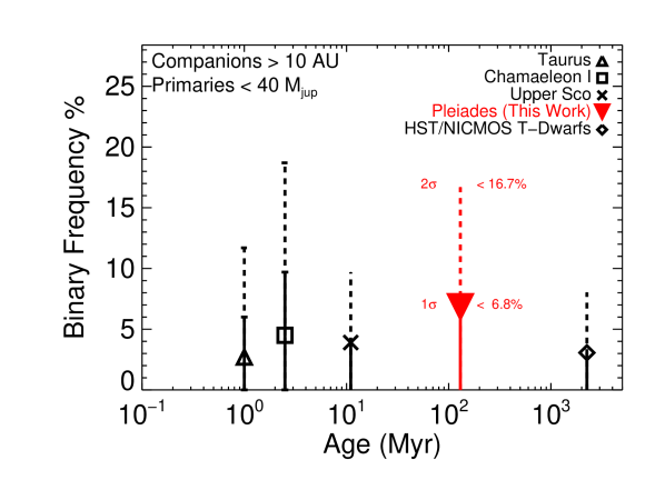
Figure 8: The wide ($>$10 AU) brown dwarf binary frequency as function of the age for young star forming regions, the intermediate age Pleiades, and the field (see §4.2). All populations are shown for a common mass range ($25-40~{}\mbox{M}_{\mbox{\tiny Jup}}$). Low mass brown dwarf binaries may very well be infrequent across a wide range of ages.

It is possible that the different cluster stellar densities in which brown dwarfs form could affect the binary frequency, hindering a direct comparison between field and young brown binary frequencies as done here. However, King et al. (2012) find that the binary frequency for stars with masses of $0.1-0.3~{}\mbox{M}_{\mbox{$\odot$}}$ did not vary measurably over nearly $20\times$ in density for five young regions (Taurus, Chamaeleon I, Ophiucus, IC 348, and the Orion Nebula Cluster). Figure 8 and Table 5 summarizes these comparisons of the binary frequency at different ages. In contrast to our estimate of the binary frequency in §4.1, here we used only the methods of Burgasser et al. (2003) for computing the binary frequency of these different clusters and the field in order to keep the statistical analysis the same.

For constraining our binary frequency of Pleiades at wider separations $a\gtrsim 10$ AU, 4 brown dwarfs observed by the HST/WFPC2 and HST/ACS surveys of Martín et al. (2003) and Bouy et al. (2006a) were combined with our own observations for a larger sample size of $15$ objects. These 4 brown dwarfs match our $K\gtrsim 16.0$ mag cutoff and conservative Pleiades cluster membership criteria, i.e. that the target must have proper motion indicating cluster membership and a spectral type $\gtrsim$M9 (see §2.1). Brown dwarfs PLIZ 28 and PLIZ 2141 were observed with HST/ACS by Bouy et al. (2006a) with detection limits that ruled out companions for mass ratios $q\gtrsim 0.45$ at separations $a\gtrsim 7-12$ AU. Brown dwarfs Roque 30 and Roque 33 were observed with HST/WFPC2 by Martín et al. (2003) and similarly they ruled out companions for mass ratios $q\gtrsim 0.5$ and separations $a\gtrsim 10$ AU. The HST/ACS and HST/WFPC2 observations have comparable detection limits to our own detection limits of $q\gtrsim 0.6$ at separations $a\gtrsim 10$ AU. Thus, with a combined sample size of 15 low mass Pleiades brown dwarfs and no binaries detected, we computed an upper limit on the binary frequency of $<$$7.0\%$ ($1\sigma$) for mass ratios $q\gtrsim 0.6$ and separations $a\gtrsim 10$ AU.

The sample of young brown dwarfs observed by HST/WFPC2 and AO surveys (see Table 5) compiled in Todorov et al. (2014) and references therein includes all targets with spectral types $\gtrsim$M4. The detection limits for these surveys are generally sensitive to companions with separations $a\gtrsim 10$ AU. In an attempt to constrain the masses of the primaries to $\lesssim$40$~{}\mbox{M}_{\mbox{\tiny Jup}}$, we included only primaries in the Todorov et al. (2014) sample with spectral types $\gtrsim$M7 (see Table 5). Note that for young ($<$10 Myr) brown dwarfs mass estimates at young ages are still uncertain and could have large uncertainties due the lack of a well measured $T_{\rm eff}$ scale for these stars and uncertain atmospheric and stellar evolution models. This spectral type cut off corresponds to a mass estimate of $\lesssim$40$~{}\mbox{M}_{\mbox{\tiny Jup}}$ at ages $\approx 1$ Myr and $\approx 2-3$ Myr for the Taurus and Chamaeleon I regions, respectively, according to the Baraffe et al. (2003) models. Over this range there are $3$ out of $37$ binaries in Taurus and $1$ out of $22$ binaries in Chamaeleon I, which corresponds to binary frequencies of $0.0-6.0$% and $0.0-10.0$% ($1\sigma$) respectively. We find our binary frequency upper limit of $<$$7.0\%$ is in agreement with binary frequencies for both Taurus and Chamaeleon I. One caveat is we included candidate companions in Taurus 2MASS J04414489+2301513 and 2MASS J04221332+1934392 from Todorov et al. (2014) in the binary frequency computed here. If those objects are not binaries, the binary frequency of Taurus would be even lower ($0.0-6.0\%$), still in agreement with our own binary frequency limit.

Kraus & Hillenbrand (2012) and Biller et al. (2011) observed 10 and 18 members of Upper Sco with spectral types $\gtrsim$M7 respectively and were sensitive to companions with separations $\gtrsim$$10$ AU. Given an age of 11 Myr for Upper Sco (Pecaut et al. 2012) and the spectral type–$T_{\rm eff}$ relation of Pecaut & Mamajek (2013), $\gtrsim$M7 spectral types correspond to $\lesssim$2650 K and thereby masses of $\lesssim$40$~{}\mbox{M}_{\mbox{\tiny Jup}}$. This is comparable to our own mass range of $25-40$ $\mbox{M}_{\mbox{\tiny Jup}}$. Both previous surveys have detection limits $q\gtrsim 0.8$ at separations $a\gtrsim 10$ AU with no binaries detected. Using this combined sample, we estimated a binary frequency of $0.0-4.0\%$ for Upper Sco, which is consistent to our own binary frequency upper limit of $<$$7.0\%$ for the Pleiades.

Burgasser et al. (2006) resolved $5$ T dwarf binaries with separations of $a=1.8-5.0$ AU out of $22$ stars observed with HST/NICMOS. They computed a Malmquist bias-corrected binary frequency of $8-19$% for mass ratios $q\gtrsim 0.6$ and separations $a\gtrsim 2$ AU. However, to directly compare to our detection limits, we recomputed their Malmquist bias-corrected binary fraction and considered only the $2$ T dwarf binaries which have projected separations of $\gtrsim$$10$ AU, which gives a binary frequency of $<$$3.0\%$ for 0 binaries detected out of $17$ objects observed.

Bate (2012) performed hydrodynamic simulations of star formation that produced 27 objects with masses $<$70 $\mbox{M}_{\mbox{\tiny Jup}}$, with none ending up as binaries. Bate (2012) quoted a binary frequency of $0.0\pm 5\%$ for the mass range of $30-70$ $\mbox{M}_{\mbox{\tiny Jup}}$ and a binary frequency of $<$7$\%$ for the mass range $10-30$ $\mbox{M}_{\mbox{\tiny Jup}}$. These predictions are in good agreement with our observed binary frequency constraint of $<$$7.0\%$ for separations $\gtrsim$$10$ AU.

5 Summary

The measurement of the brown dwarf binary frequency at different ages is fundamental tool for testing theory, given that the statistical properties of binaries probe formation scenarios in the very low-mass regime. In this work, we tripled the number low-mass Pleiades brown dwarfs searched for companions, surveying a sample of 11 previously unobserved L dwarfs in the Pleiades, predecessors to T dwarfs in the field, using HST/WFC3. We have constrained the binary frequency in Pleiades for the lowest known mass ($25-40$ $\mbox{M}_{\mbox{\tiny Jup}}$) and latest known type ($\gtrsim$M9) brown dwarfs to $<$$11\%$ at $1\sigma$ ($<$$26\%$ at $2\sigma$) confidence for companions as close as $\approx 4$ AU, finding no binaries. Our survey is the first to probe down to separations of $4$ AU at such young ages.

Furthermore, we find our binary frequency constraints are in good agreement with observed binary frequencies of young star forming regions Taurus ($0.0-6.0$%), Chamaeleon I ($0.0-10.0$%), and Upper Sco ($0.0-4.0$%) for objects with similar primary masses of $<$40 $\mbox{M}_{\mbox{\tiny Jup}}$, at $1\sigma$ with projected separations $>$10 AU. Overall, our observations of the Pleiades support the evidence that T dwarf binaries are likely uncommon, and consistent with having the same frequency at both young ($1-10$ Myr), intermediate ($\approx$$120$ Myr) and old ($\gtrsim$$1$ Gyr) ages.

Table 1: Pleiades Sample

Namea	R. A.	Decl.	Massb	K	SpT	SpT	P.M.
	J2000.0	J2000.0	$\mbox{M}_{\mbox{\tiny Jup}}$	mag		Ref	Ref
BRB 17	03 54 07.98	+23 54 27.9	43	$16.03\pm 0.03$	L0	1	2
NPNPL 2	03 46 34.26	+23 50 03.7	41	$16.09\pm 0.03$			3
PLIZ 31	03 51 47.65	+24 39 59.2	40	$16.09\pm 0.03$			3,4
BRB 21	03 54 10.27	+23 41 40.2	31	$16.39\pm 0.04$	L3	1	2
PLIZ 35	03 52 39.16	+24 46 29.5	31	$16.51\pm 0.04$	L2	1	2
BRB 23	03 50 39.54	+25 02 54.7	30	$16.56\pm 0.04$	L3.5	1	2
PLIZ 161	03 51 29.47	+24 00 37.3	28	$16.70\pm 0.05$			3
UGCS J0348+2550e	03 48 15.63	+25 50 08.9	28	$16.73\pm 0.05$	L3$\pm$1	8	3,7
BRB 28	03 52 54.90	+24 37 18.2	26	$16.92\pm 0.06$			2
PLIZ 1262	03 44 27.27	+25 44 42.0	26	$16.95\pm 0.07$			2,4
BRB 29	03 54 01.43	+23 49 57.7	25	$17.00\pm 0.07$	L4.5	1	2
Roque 33c	03 48 49.03	+24 20 25.4	41	$16.06\pm 0.03$	M9.5	6	5
Roque 30c	03 50 16.09	+24 08 34.7	40	$16.08\pm 0.03$			3
PLIZ 28d	03 54 14.03	+23 17 51.4	35	$16.14\pm 0.03$	L0.0	1	2
PLIZ 2141d	03 44 31.29	+25 35 14.4	28	$16.69\pm 0.04$			2

Note. — ^a To search these targets by name in Simbad, add the string “Cl* Melotte 22”

^b Masses are estimated from Baraffe et al. (2003)

^c Observed with HST/WFPC2 Martín et al. (2003)

^d Observed with HST/ACS Bouy et al. (2006a)

^e UGCS J$034815.64+255008.9$

References. (1) Bihain et al. (2010); (2) Bihain et al. (2006); (3) Lodieu et al. (2012); (4) Casewell et al. (2007); (5) Stauffer et al. (2007); (6) Martín et al. (2000) (7) Zapatero Osorio et al. (2014a); (8) Zapatero Osorio et al. (2014b)

Table 2: HST/WFC3 Photometry

Our Targets	F814W	F850LP
	(mag)	(mag)
BRB 17	$20.419\pm 0.007$	$19.415\pm 0.011$
NPNPL 2	$20.685\pm 0.006$	$19.448\pm 0.011$
PLIZ 31	$20.701\pm 0.006$	$19.524\pm 0.013$
BRB 21	$21.344\pm 0.010$	$20.204\pm 0.023$
PLIZ 35	$21.315\pm 0.010$	$20.096\pm 0.021$
BRB 23	$21.604\pm 0.012$	$20.431\pm 0.029$
PLIZ 161	$21.804\pm 0.014$	$20.678\pm 0.034$
UGCS J0348+2550	$21.866\pm 0.015$	$20.706\pm 0.035$
BRB 28	$22.177\pm 0.019$	$20.860\pm 0.040$
PLIZ 1262	$22.211\pm 0.020$	$21.086\pm 0.049$
BRB 29	$22.231\pm 0.021$	$21.042\pm 0.048$

Table 3: Binary Simulations

Simulation	Filter	S/N	Number of
			Artificial Binaries
Median S/N	F814W	93.5	$4800$
Min S/N	F814W	61.1	$4800$
Median S/N	F850LP	49.1	$4800$
Min S/N	F850LP	33.0	$4800$

Table 4: Detection Limits

Target	$0\farcs 025$	$0\farcs 032$	$0\farcs 040$	$0\farcs 050$	$0\farcs 063$	$0\farcs 080$	$0\farcs 100$	$0\farcs 126$	$0\farcs 159$	$0\farcs 180$
F814W (mag)
BRB17	20.66	21.26	21.88	22.20	22.48	22.75	22.77	23.05	23.69	23.06
NPNPL2	20.93	21.52	22.15	22.46	22.75	23.02	23.04	23.31	23.95	23.33
PLIZ31	20.94	21.54	22.17	22.48	22.76	23.03	23.05	23.33	23.97	23.35
BRB21	21.59	22.18	22.81	23.12	23.41	23.67	23.70	23.97	24.61	23.99
PLIZ35	21.56	22.15	22.78	23.09	23.38	23.65	23.67	23.94	24.58	23.96
BRB23	21.85	22.44	23.07	23.38	23.67	23.93	23.96	24.23	24.87	24.25
PLIZ161		22.64	23.27	23.26	23.54	24.13	23.86	24.43	24.72	24.45
UGCSJ0348+2550		22.70	23.33	23.32	23.61	23.93	23.92	24.49	24.78	24.51
BRB28		22.70	23.30	23.63	23.92	24.25	24.23	24.53	24.76	24.55
PLIZ1262		22.73	23.34	23.66	23.66	24.28	24.27	24.57	24.80	24.58
BRB29		22.75	23.36	23.68	23.68	24.30	24.29	24.59	24.82	25.44
F850LP (mag)
BRB17			20.26	20.55	20.57	20.90	21.49	21.14	21.77	21.76
NPNPL2			20.29	20.59	20.60	20.93	21.52	21.17	21.81	21.80
PLIZ31			20.37	20.66	20.68	21.01	21.60	21.25	21.88	21.87
BRB21			21.05	21.34	21.36	21.69	22.28	21.93	22.56	22.55
PLIZ35			20.94	21.23	21.25	21.58	22.17	21.82	22.46	22.44
BRB23			21.28	21.57	21.59	21.91	22.51	22.16	22.79	22.78
PLIZ161			20.73	20.92	21.83	22.16	22.12	22.40	22.44	22.16
UGCS J0348+2550			20.76	20.95	21.86	22.19	22.15	22.43	22.46	22.19
BRB28				20.91	21.71	22.02	22.31	22.30	22.30	22.34
PLIZ1262				21.14	21.94	22.24	22.53	22.53	22.53	22.57
BRB29				21.10	21.90	21.88	22.49	22.48	22.48	22.53

Table 5: Binary Frequency vs. Age for Wide ($>$10) AU Companions

Region	Age	Age	Sample	$N_{\rm obj}$	$N_{\rm bin}$	Bin Freq	$q$
		Ref	Ref			%
Taurus	1 Myr	15	1,2,3,4,5	37	3	$0.0-6.0$	$\gtrsim 0.7$
Chameleon I	2-3 Myr	16	4,5,6,7,8,9,10	22	1	$0.0-10.0$	$\gtrsim 0.7$
Upper Sco	11 Myr	17	2,11	28	0	$0.0-4.0$	$\gtrsim 0.8$
This work + lit	125 Myr	18	12,13	15	0	$<$$7.0$	$\gtrsim 0.6$
Field	0.5-5.0 Gyr	19	14	17	0	$<$$3.0$	$\gtrsim 0.6$

Note. — Faint companions to brown dwarfs with separations and mass ratios greater than given in table are ruled out by the given detection limits for primaries with masses $<$40$\mbox{M}_{\mbox{\tiny Jup}}$ and separations $>$10 AU.

References. (1) Todorov et al. (2014); (2) Kraus & Hillenbrand (2012); (3) Kraus et al. (2006)(4) Konopacky et al. (2007) (5) Todorov et al. (2010); (6) Luhman (2004); (7) Lafrenière et al. (2008); (8) Ahmic et al. (2007); (9) Luhman (2007); (10) Neuhäuser et al. (2002); (11) Biller et al. (2011); (12) Martín et al. (2003); (13) Bouy et al. (2006a); (14) Burgasser et al. (2006); (15) Luhman (2007); (16) Luhman et al. (2010); (17) Pecaut et al. (2012); (18) Barrado y Navascués et al. (2004); (19) Assumed age for field T dwarfs by Burgasser et al. (2006) from Reid & Hawley (2000).

Table 6: Companion Detectability

Name	Detectability
	log normal $a$
BRB17	$70.8$%
BRB21	$68.7$%
BRB23	$69.9$%
BRB28	$67.2$%
BRB29	$66.7$%
NPNPL2	$71.4$%
PLIZ1262	$66.9$%
PLIZ161	$68.8$%
PLIZ31	$71.3$%
PLIZ35	$68.6$%
UGCS J0348+2550	$68.8$%
Total Expected Binaries	$7.6$
Binary Frequencya	$<$$11$%

Note. — ^a Binary frequency with $1\sigma$ using the Jeffrey interval recommended for low $n$ by Brown et al. (2001).

References

- Aberasturi et al. (2014) Aberasturi, M., Burgasser, A. J., Mora, A., et al. 2014, AJ, 148, 129
- Ahmic et al. (2007) Ahmic, M., Jayawardhana, R., Brandeker, A., et al. 2007, ApJ, 671, 2074
- Allen (2007) Allen, P. R. 2007, ApJ, 668,492
- Allers et al. (2006) Allers, K. N., Kessler-Silacci, J. E., Cieza, L. A., & Jaffe, D. T. 2006, ApJ, 644, 364
- Allard (2014) Allard, F. 2014, IAU Symposium, 299, 271
- Barrado y Navascués et al. (2004) Barrado & Navascués, D., Stauffer, J. R., & Jayawardhana, R. 2004, ApJ, 614, 386
- Baraffe et al. (1997) Baraffe, I., Chabrier, G., Allard, F., & Hauschildt, P. H. 1997, A&A, 327, 1054
- Baraffe et al. (1998) Baraffe, I., Chabrier, G., Allard, F., & Hauschildt, P. H. 1998, A&A, 337, 403
- Baraffe et al. (2003) Baraffe, I., Chabrier, G., Barman, T. S., Allard, F., & Hauschildt, P. H. 2003, A&A, 402, 701
- Bate (2009) Bate, M. R. 2009, MNRAS, 392, 590
- Bate (2012) Bate, M. R. 2012, MNRAS, 419, 3115
- Bihain et al. (2006) Bihain, G., Rebolo, R., Béjar, V. J. S., et al. 2006, A&A, 458, 805
- Bihain et al. (2010) Bihain, G., Rebolo, R., Zapatero Osorio, M. R., Béjar, V. J. S., & Caballero, J. A. 2010, A&A, 519, A93
- Biller et al. (2011) Biller, B., Allers, K., Liu, M., Close, L. M., & Dupuy, T. 2011, ApJ, 730, 39
- Bouy et al. (2003) Bouy, H., Brandner, W., Martín, E. L., et al. 2003, AJ, 126, 1526
- Bouy et al. (2006a) Bouy, H., Moraux, E., Bouvier, J., et al. 2006, ApJ, 637, 1056
- Bouy et al. (2006b) Bouy, H., Martín, E. L., Brandner, W., et al. 2006, A&A, 451, 177
- Brown et al. (2001) Brown, LD, Cat, TT and DasGupta, A (2001). Interval Estimation for a Binomial proportion. Statistical Science 16:101-133
- Burgasser et al. (2003) Burgasser, A. J., Kirkpatrick, J. D., Reid, I. N., et al. 2003, ApJ, 586, 512
- Burgasser et al. (2006) Burgasser, A. J., Kirkpatrick, J. D., Cruz, K. L., et al. 2006, ApJS, 166, 585
- Burgasser et al. (2007) Burgasser, A. J., Reid, I. N., Siegler, N., et al. 2007, Protostars and Planets V, 427
- Burningham et al. (2010) Burningham, B., Pinfield, D. J., Lucas, P. W., et al. 2010, MNRAS, 406, 1885
- Burningham et al. (2013) Burningham, B., Cardoso, C. V., Smith, L., et al. 2013, MNRAS, 433, 457
- Casewell et al. (2007) Casewell, S. L., Dobbie, P. D., Hodgkin, S. T., et al. 2007, MNRAS, 378, 1131
- Chiu et al. (2006) Chiu, K., Fan, X., Leggett, S. K., et al. 2006, AJ, 131, 2722
- Cushing et al. (2011) Cushing, M. C., Kirkpatrick, J. D., Gelino, C. R., et al. 2011, ApJ, 743, 50
- Close et al. (2007) Close, L. M., Zuckerman, B., Song, I., et al. 2007, ApJ, 660, 1492
- Delfosse et al. (1997) Delfosse, X., Tinney, C. G., Forveille, T., et al. 1997, A&A, 327, L25
- Dobbie et al. (2002) Dobbie, P. D., Kenyon, F., Jameson, R. F., et al. 2002, MNRAS, 335, 687
- Duchêne et al. (2013) Duchêne, G., Bouvier, J., Moraux, E., et al. 2013, A&A, 555, A137
- Dupuy & Liu (2011) Dupuy, T. J., & Liu, M. C. 2011, ApJ, 733, 122
- Epchtein et al. (1997) Epchtein, N., de Batz, B., Capoani, L., et al. 1997, The Messenger, 87, 27
- Gelino et al. (2011) Gelino, C. R., Kirkpatrick, J. D., Cushing, M. C., et al. 2011, AJ, 142, 57
- Jameson et al. (2002) Jameson, R. F., Dobbie, P. D., Hodgkin, S. T., & Pinfield, D. J. 2002, MNRAS, 335, 853
- King et al. (2012) King, R. R., Parker, R. J., Patience, J., & Goodwin, S. P. 2012, MNRAS, 421, 2025
- Konopacky et al. (2007) Konopacky, Q. M., Ghez, A. M., Rice, E. L., & Duchêne, G. 2007, ApJ, 663, 394
- Kraus et al. (2005) Kraus, A. L., White, R. J., & Hillenbrand, L. A. 2005, ApJ, 633, 452
- Kraus et al. (2006) Kraus, A. L., White, R. J., & Hillenbrand, L. A. 2006, ApJ, 649, 306
- Kraus & Hillenbrand (2007) Kraus, A. L., & Hillenbrand, L. A. 2007, AJ, 134, 2340