Ecological collapse and the emergence of traveling waves at the onset of shear turbulence

Abstract

The transition to turbulence exhibits remarkable spatio-temporal behavior that continues to defy detailed understanding. Near the onset to turbulence in pipes, transient turbulent regions decay either directly or, at higher Reynolds numbers through splitting, with characteristic time-scales that exhibit a super-exponential dependence on Reynolds number. Here we report numerical simulations of transitional pipe flow, showing that a zonal flow emerges at large scales, activated by anisotropic turbulent fluctuations; in turn, the zonal flow suppresses the small-scale turbulence leading to stochastic predator-prey dynamics. We show that this “ecological” model of transitional turbulence reproduces the super-exponential lifetime statistics and phenomenology of pipe flow experiments. Our work demonstrates that a fluid on the edge of turbulence is mathematically analogous to an ecosystem on the edge of extinction, and provides an unbroken link between the equations of fluid dynamics and the directed percolation universality class.

Introduction.

Fluids in motion are generally found in one of two generic states. The most common — turbulence — is found at sufficiently large characteristic speeds $U$, depending on the kinematic viscosity $\nu$ and the characteristic system scale $D$; turbulent flows are complex, stochastic, and unpredictable in detail. At lower velocities, the fluid is said to be laminar: its flow is simple, deterministic and predictable. In between these two states, conventionally delineated by the dimensionless control parameter known as the Reynolds number $\hbox{Re}\equiv UD/\nu$, is a transitional regime that occurs for $1700\lesssim\hbox{Re}\lesssim 2300$ in pipes, and which has presented a challenge to experiment and theory since Osborne Reynolds’ original observation of intermittent “flashes” of turbulence Reynolds (1883). Today, Reynolds’ flashes are known as puffs Wygnanski and Champagne (1973), and their behavior has been characterized very precisely through a series of physical and numerical experiments performed during the last decade or so Faisst and Eckhardt (2004); Peixinho and Mullin (2006); Hof et al. (2006); Willis and Kerswell (2007) (for a recent review, see Song and Hof (2014)) culminating in the tour de force observation of a super-exponential functional dependence of the lifetime $\tau^{d}$ of puffs as a function of Re Hof et al. (2008): $\ln\ln\tau^{d}\propto\hbox{Re}$. For Reynolds numbers based upon pipe diameter $D$ of around 2300, turbulence is sustained longer than the ability to observe its lifetime in finite systems, and the puffs become unstable through a new dynamical processes in which the leading edge breaks away and nucleates the formation of a new puff some distance downstream Wygnanski et al. (1975); Moxey and Barkley (2010); Avila et al. (2011); Nishi et al. (2008). The puff-splitting occurs on a characteristic time that decays super-exponentially with increasing Re. These phenomena are likely to be generic. For example, super-exponential scaling behavior near the transition to turbulence has also been reported in plane Poiseuille flow Lemoult et al. (2014) and Taylor-Couette flow Borrero-Echeverry et al. (2010). In addition, optical analogues of the laminar-turbulence transition have been observed in laser-driven optical fibers Turitsyna et al. (2013).

The theoretical account of these phenomena has focused primarily on the existence and interactions between nonlinear solutions of the Navier-Stokes equations, periodic orbits and streamwise vortices Willis et al. (2013); Cvitanović (2013); Avila et al. (2013); Kerswell (2005); Eckhardt et al. (2007); Chantry et al. (2014), and the dynamics of long-lived chaotic transients Crutchfield and Kaneko (1988). An alternative line of inquiry has been to characterize the statistical properties of transitional turbulence through ad hoc model equations. These have been motivated either by perceptive analogies to excitable media Barkley (2011) or by phase transition universality arguments that begin with the notion that the laminar state is an absorbing one Pomeau (1986), and show quantitatively how super-exponential decay results from the generic universality class for non-equilibrium absorbing processes Janssen (1981): directed percolation (DP) Sipos and Goldenfeld (2011). Both approaches reflect an important aspect of the dynamics, namely that a certain minimum level of energy is required to sustain turbulent puffs Peixinho and Mullin (2007), leading to a further connection with extreme value statistics Goldenfeld et al. (2010).

It is the statistical behavior near the transition which concerns us here: how do the various spatial-temporal modes that are excited give rise to such remarkable lifetime statistics? What is the universality class of this transition, in terms of its fluctuation characteristics? Are there simplified effective descriptions that bridge the gap between the underlying fluid dynamics and the large-scale statistical properties? And how do these emerge from the underlying Navier-Stokes equations that govern all hydrodynamic phenomena?

The purpose of this report is to address these questions using the same approach by which phase transitions are understood in condensed matter physics Goldenfeld (1992). There it is well-established that universal aspects of phase transitions, such as the phase diagram, critical exponents, scaling functions etc. are all described quantitatively by an effective coarse-grained theory (“Landau theory”) that contains the symmetry-allowed collective and long-wavelength modes, without requiring excessive realism at the microscopic level of description. Being based on symmetry principles, the individual symmetry-allowed terms in Landau theory do not require detailed derivation from the microscopic level of description. This is fortunate given that there is usually no good, uniformly valid approximation scheme to derive formally and systematically these terms and their coefficients from first principles.

For the transitional turbulence problem, the analytical difficulties are acute. Therefore, in this paper, we avoid approximations which are difficult to justify systematically. Instead, we use direct numerical simulation to identify the important collective modes which exhibit an interplay between large-scale fluctuations and small-scale dynamics at the onset of turbulence, and thence to write down the corresponding minimal stochastic model, in the spirit of the Landau theory of phase transitions. As we will show, this coarse-grained description is able to account for the principal experimental observations and to predict quantitatively the puff lifetime and splitting behavior observed near the transition. Our stochastic model can be transformed using standard statistical mechanics techniques into a field theory known to be in the universality class of directed percolation. These results provide an unbroken link between the equations of fluid dynamics and the directed percolation universality class Pomeau (1986); Sipos and Goldenfeld (2011). Our approach is thus a precise parallel to the way in which phase transitions are understood in condensed matter physics, and shows that concepts of universality and effective theories are applicable to the laminar-turbulence transition.

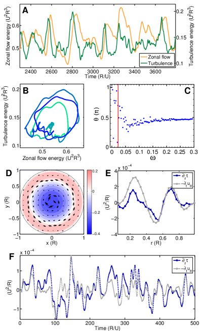
Figure 1: Predator-prey oscillations in transitional turbulent pipe flow. (A) Energy vs. time for the zonal flow (orange) and turbulent modes (green). (B) Phase portrait of the zonal flow and turbulent modes as a function of time, with color indicating the earliest time in dark blue progressing to the latest time in light green. (C) Phase shift between the turbulent and zonal flow modes as a function of frequency, showing that the turbulence leads the zonal flow by $~{}\pi/2$ consistent with predator-prey dynamics. The phase shift $\theta\left(\omega\right)=\tan^{-1}\left(Im[\tilde{C}(\omega)]/Re[\tilde{C}(\omega)]\right)$ and is shifted to be positive, where $\tilde{C}(\omega)$ is the Fourier transform of the correlation function between the turbulence and the zonal flow in (A). The red line corresponds to the dominant frequency in the power spectrum. The phase shift near small $\omega$ is scatter due to the finite time duration of the time series. (D) Velocity field configuration of the zonal flow mode $\vec{\overline{u}}$. The color bar indicates the value of $\overline{u}_{z}$. (E) Snapshot of the Reynolds stress gradient and zonal flow time-derivative as functions of $r$. (F) Reynolds stress gradient and zonal flow time derivative as functions of time. The evident proportionality shows that zonal flow dynamics is driven by the radial gradient of the Reynolds stress.

Observation of predator-prey dynamics in Navier-Stokes equations.

To address these questions without making questionable or non-systematic approximations, we have performed direct numerical simulations (DNS) of the Navier-Stokes equations in a pipe, using the open-source code “Open Pipe Flow” Willis and Kerswell (2009), as described in Appendix A. We denote the time-dependent velocity deviation from the Hagen–Poiseuille flow by $\vec{u}=(u_{z},u_{\theta},u_{r})$. Because we were interested in transitional behavior, we looked for a decomposition Prigent et al. (2002); Moxey and Barkley (2010); Duguet and Schlatter (2013); Lemoult et al. (2014) of large-scale modes that would indicate some form of collective behavior, as well as small-scale modes that would be representative of turbulent dynamics In particular, we report here the behavior of the velocity field $(\overline{u}_{z},\overline{u}_{\theta},\overline{u}_{r})$, where the bar denotes average over $z$ and $\theta$, and $\overline{u}_{r}=0$. We refer to this as the zonal flow (ZF). In Fourier space, the zonal flow is given by $\tilde{\vec{u}}(k=0,m=0,r)$, where $k$ is the axial wavenumber and $m$ is the azimuthal wavenumber, $r$ is the real space radial coordinate and the tilde denotes Fourier transform in the $\theta$ and $z$ directions only. Turbulence was represented by short-wavelength modes, whose energy is $E_{T}(t)\equiv\frac{1}{2}\sum_{|k|\geq 1,|m|\geq 1}\int|\tilde{\vec{u}}(k,m,r)|^{2}\,\text{d}V$.

Shown in Figure 1(A) is a time series for the energy $E_{ZF}(t)$ of the zonal flow, compared with the energy $E_{T}(t)$ of the turbulent energy. The curves show clear persistent oscillatory behavior, modulated by long-wavelength stochasticity as shown in the phase portrait of Figure 1(B). In Figure 1(C), we have calculated the phase shift between the turbulence and zonal flows, with the result that the turbulent energy leads the zonal flow energy by $\sim\pi/2$. This suggests that these oscillations can be interpreted as a time-series resulting from activator-inhibitor dynamics, such as occurs in a predator-prey ecosystem. Predator-prey ecosystems are characterized by the following behavior: the “prey” mode activates the “predator” mode, which then grows in abundance. At the same time, the growing predator mode begins to inhibit the prey mode. The inhibition of the prey mode starves the predator mode, and it too becomes inhibited. The inhibition of the predator mode allows the prey mode to re-activate, and the population cycle begins again.

The flow configuration for the predator mode is shown in Figure 1 (D), and consists of a series of azimuthally symmetric modes with direction reversals as a function of radius $r$. Such banded shear flows are known as zonal flows and are of special significance in plasma physics, astrophysical and geophysical flows, owing to their role in regulating turbulence Diamond et al. (1994). The purely azimuthal component of the zonal flow, denoted by $\overline{u}_{\theta}(r)$ is spatially uniform in $z$, and the lack of a radial component means that it is not driven by pressure gradients. Thus it can only exist due to nonlinear interactions with turbulent modes. In this sense, it is a collective mode, one with special significance for transitional turbulence.

The simplest way for such an azimuthal shear flow to couple to turbulent fluctuations is through the Reynolds stress $\tau$: however, a uniform Reynolds stress cannot drive a shear flow, so the first symmetry-allowed possibility is the radial gradient of the Reynolds stress Diamond et al. (1994), as expressed in the Reynolds momentum equation. Thus, to probe the dynamics that govern the emergence of the zonal flow, we have calculated the time-averaged radial gradient of the instantaneous Reynolds stress, $\tau\equiv u^{\prime}_{\theta}\cdot u^{\prime}_{r}$, where $\vec{u^{\prime}}(z,\theta,r)\equiv\vec{u}-\vec{\overline{u}}$, and show in Figure 1 (F) the 4.5-time-unit-running-mean time series of $-\partial_{t}\overline{u}_{\theta}$ and the radial gradient $\partial_{r}\tau$. Both quantities have been averaged over $0\leq z\leq L$, $0\leq\theta\leq 2\pi$ and $R_{0}\leq r<R$, where $R_{0}=0.641R$, and the resulting time series are clearly highly correlated.

In general, it is the case that zonal flows are driven by statistical anisotropy in turbulence, but are themselves an isotropizing influence on the turbulence through their coupling to the Reynolds stress Sivashinsky and Yakhot (1985); Bardóczi et al. (2014); Parker and Krommes (2014). The fact that turbulence anisotropy activates the zonal flow, and that zonal flow inhibits the turbulence is responsible for the predator-prey oscillations observed in the numerical simulations.

Lifetime of stochastic predator-prey populations.

Phase transition theory Goldenfeld (1992) would suggest that the emergence of a zonal flow collective mode dominates the non-equilibrium transition of pipe flow from the laminar to the turbulent state, through the predator-prey interaction with the small scale velocity fluctuations. Such a “two fluid” effective field description of transitional turbulence implies that stochastic predator-prey populations should undergo spatio-temporal fluctuations whose functional form matches precisely the observations for the lifetime and splitting time of turbulent puffs in a pipe. To test this idea, we have performed simulations of a spatially-extended stochastic predator-prey ecosystem, in a quasi-one-dimensional geometry to mimic the pipe environment. The specific system has three trophic levels: nutrient (E), Prey (B) and Predator (A), which correspond in the fluid system to laminar flow, turbulence and zonal flow respectively. The interactions between individual representatives of these levels are given by the following rate equations

$$A_{i}\xrightarrow{\textit{$d_{A}$}}E_{i},\qquad B_{i}\xrightarrow{\textit{$d_{B}$}}E_{i},\qquad A_{i}+B_{j}\xrightarrow[\langle ij\rangle]{\textit{$p$}}A_{i}+A_{j},$$

$$B_{i}+E_{j}\xrightarrow[\langle ij\rangle]{\textit{$b$}}B_{i}+B_{j},\qquad B_{i}\xrightarrow{\textit{$m$}}A_{i},$$

$$A_{i}+E_{j}\xrightarrow[\langle ij\rangle]{\textit{$D$}}E_{i}+A_{j},\;\;\;B_{i}+E_{j}\xrightarrow[\langle ij\rangle]{\textit{$D$}}E_{i}+B_{j}.$$ (1)

where $d_{A}$ and $d_{B}$ are the death rates of A and B, $p$ is the predation rate, $b$ is the prey birth rate due to consumption of nutrient, $\langle ij\rangle$ denotes hopping to nearest neighbor sites, $D$ is the nearest-neighbor hopping rate, and $m$ is the point mutation rate from prey to predator, which models the induction of the zonal flow from the turbulence degrees of freedom.

We are primarily interested in long-wavelength properties of the system, at least in the vicinity of the turbulence transition, where we expect the transverse correlation length to be larger than the pipe diameter, implying that the behavior is in fact quasi-one-dimensional. The crossover phenomena associated with this have been discussed previously Sipos and Goldenfeld (2011), and thus our quasi-one-dimensional model should be appropriate and quantitatively correct near the transition.

In our simulation, described in Appendix B, the control parameter is the prey birth rate $b$. When $b$ is small enough, the population is metastable, and cannot sustain itself: all individuals, both predator and prey, eventually die within a finite lifetime $\tau^{d}(b)$. As $b$ increases, the lifetime of the population increases rapidly: in particular the prey lifetime increases rapidly with $b$. At large enough values of $b$, the decay of the initial population is not observed, but instead the initially localized population proliferates, spreading outwards and spontaneously splitting into multiple clusters, as shown in the space-time plot of clusters of prey of Figure 2 (A).

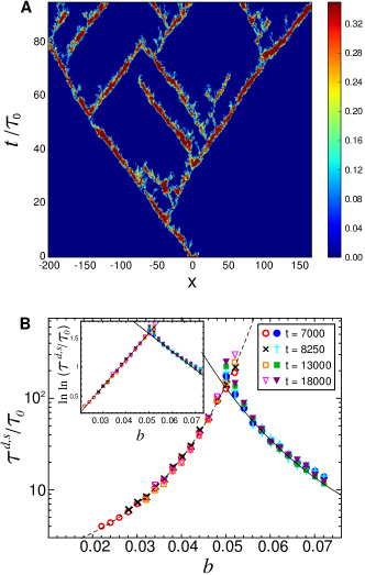
Figure 2: Stochastic predator-prey model reproduces the phenomenology of transitional pipe turbulence. Decay lifetime, $\tau^{d}$, and splitting time, $\tau^{s}$, of clusters of prey are memoryless processes and obey super-exponential statistics as a function of prey birth rate. To compare with the experiments Hof et al. (2008), predator-prey dynamics are performed in two-dimensional pipe geometry as described in the text. (A) World line of clusters of prey splitting to form predator-prey traveling waves. The color measures the local density of prey, corresponding to intensity of turbulence in pipe flow. In the simulation, the dimensionless parameters are $D=0.1$, $b=0.1$, $p=0.2$, $d_{A}=0.01$, $d_{B}=0.01$ and $m=0.001$. In the model simulated, diffusion is isotropic, not biased as would be the case corresponding to a mean flow, where the clusters will accumulate at large times with a well-defined separation set by the depletion zone of nutrient behind each predator-prey traveling wave. (B) Log decay lifetime of prey cluster and splitting time as a function of prey birth rate. The upward curvature signifies super-exponential behavior. The parameters are $D=0.01$, $p=0.1$, $d_{A}=0.015$, $d_{B}=0.025$ and $m=0.001$. Inset: Double log lifetime vs prey birth rate, showing the fit to the following functional forms: the dashed curve is given by $\tau^{d}/\tau_{0}=\exp(\exp(46.539b-0.731))$, and the solid curve is given by $\tau^{s}/\tau_{0}=\exp(\exp(-31.148b-3.141))$.

To quantify these observations, we have measured both the lifetime of population clusters in the metastable region and their splitting time using a procedure directly following that of the turbulence experiments and simulations Avila et al. (2011), and described in Appendix C. We comment that both timescales involve implicitly measurements of quantities that exceed a given threshold, and thus it is natural that the results are found to conform to extreme value statistics Goldenfeld et al. (2010); Sipos and Goldenfeld (2011).

In Figure 2 (A) we show the phenomenology of the dynamics of initial clusters of prey, corresponding to the predator-prey analogue for the experiments in pipe flow which followed the dynamics of an initial puff of turbulence injected into the flow Hof et al. (2008). Depending upon the prey birth rate, the cluster decays either homogeneously or by splitting, precisely mimicking the behavior of turbulent puffs as a function of Reynolds number. The extraction from data of decay times is described in Appendix C. In Figure 2 (B) is shown the semi-log plot of lifetime for both decay and splitting as a function of prey birth rate, the upward curvature indicative of super-exponential behavior. The inset to Figure 2 (B) shows a double exponential plot of puff lifetime and splitting time vs. prey birth rate, the straight line being the fit to the functional form indicated in the caption. These figures indicate a remarkable similarity to the corresponding plots obtained for transitional pipe turbulence in both experiments Hof et al. (2008) and direct numerical simulations Avila et al. (2011), and demonstrate conclusively that experimental observations are well captured by an effective two-fluid model of pipe flow turbulence with predator-prey interactions between the zonal flow and the small scale turbulence.

Universality class of the laminar-turbulence transition in pipes.

The two-fluid predator-prey model expressed by Equations (1) exhibits a rich phase diagram that captures the main features observed in transitional turbulence in pipes. The transition to puff-splitting can be identified with a change of stability of the spatially-uniform mean-field predator-prey coexistence point, where a stable node becomes a stable focus or spiral with increasing birth rate. In the language of predator-prey systems, this corresponds to the breakdown of spatially homogeneous prey domains into periodic traveling wave states. The phase diagram is sketched in Figure 3, along with the corresponding phase diagram for transitional pipe turbulence as determined by experiment. The phenomenology of the predator-prey system mirrors that of turbulent pipe flow.

In order to determine the universality class of the non-equilibrium phase transition from laminar to turbulent flow, we use the two-fluid predator-prey mode in Equations (1). Near the transition to prey extinction, the prey population is very small and no predator can survive, and thus Equations (1) simplify to

$$B_{i}\xrightarrow{\textit{$d_{B}$}}E_{i},\qquad B_{i}+E_{j}\xrightarrow[\langle ij\rangle]{\textit{$b$}}B_{i}+B_{j},$$

$$B_{i}+E_{j}\xrightarrow[\langle ij\rangle]{\textit{$D$}}E_{i}+B_{j}.$$ (2)

These equations are exactly those of the reaction-diffusion model for directed percolation Ódor (2004). A more detailed and systematic way to reach this conclusion is to represent Equations 1 exactly in path integral form using the Doi formalism Doi (1976); Grassberger and Scheunert (1980); Mikhailov (1981); Goldenfeld (1984); Mattis and Glasser (1998); Ódor (2004). The resulting action simplifies near the transition to that of Reggeon field theory Mobilia et al. (2007); Täuber (2012), which has been shown to be in the universality class of directed percolation Cardy and Sugar (1980); Janssen (1981). Numerical simulations of 3 + 1 dimensional directed percolation in a pipe geometry have reproduced the statistics and behavior of turbulent puffs and slugs in pipe flow Sipos and Goldenfeld (2011); Allhoff and Eckhardt (2012), and a detailed comparison between theory and experiment has been presented Shi et al. (2015). The super-exponential behavior of DP might seem to contradict the expectation based upon the known critical behavior (e.g., see Ref. Hinrichsen (2000)). However, it is important to recognize that the usual exponents relate to DP starting from a single seed, whereas the experiments and simulations are conducted with an extended seed that has a finite length or number of seed points. These points behave as independent identically-distributed random variables as long as the transverse correlation length is much smaller than the seed size, but once the correlation length is of order the seed size, the seed is effectively a single correlated extended source, and once the correlation length is much larger than this size, there will be a crossover to the usual DP exponents.

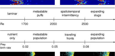
Figure 3: Schematic phase diagram for transitional pipe turbulence as a function of Reynolds number compared with the phase diagram for predator-prey dynamics as a function of prey birth rate. Above each phase is shown a typical flow or predator-prey configuration, indicating the similarity between the turbulent pipe and ecosystem dynamics.

Discussion.

The observation of the emergence of a zonal flow, excited by the developing turbulent degrees of freedom and the demonstration of its role in determining the phenomenology of transitional pipe turbulence has an interesting consequence: the zonal flow can be assisted by rotating the pipe, and this should catalyze the transition to turbulence, causing it to occur at lower Re. Indeed experiments on axially-rotating pipes Murakami and Kikuyama (1980) are consistent with this prediction.

The idea that predator-prey dynamics can arise in turbulence is by no means new, and such behavior was proposed by Diamond and collaborators Diamond et al. (1994); Kim and Diamond (2003); Itoh et al. (2006) many years ago in the context of the interaction between drift-wave turbulence and zonal flows in tokomaks; indeed the predator-prey oscillations were recently observed in tokomaks Estrada et al. (2010); Conway et al. (2011); Xu et al. (2011); Estrada et al. (2011); Schmitz et al. (2012) and in a table-top electroconvection analogue of the L-H transition Bardóczi et al. (2014). The new ingredient we have presented in this paper is the observation of a zonal flow emerging in the very simple setting of transitional pipe turbulence, and the demonstration of predator-prey oscillations that suggest a minimal mesoscale model of transitional turbulence that accounts for the observed statistical behavior of puffs. The logic of our work is that we used DNS to identify the important collective modes at the onset of turbulence—the predator-prey modes—and then wrote down the simplest minimal stochastic model to account for these observations. This model predicts without using the Navier-Stokes equations the puff lifetime and splitting behavior observed in experiment. This approach is a precise parallel to that used in the conventional theory of phase transitions, where one builds a Landau theory, a coarse-grained (or effective) theory, using symmetry principles. This intermediate level description can then be used as a starting point for renormalization group analysis to compute the critical behavior.

Note that it is neither necessary nor desirable to derive the coarse-grained effective theory from the microscopic description. Such a derivation is not necessary, because any such derivation would need a small parameter and would thus only have limited validity due to the analytical approximations made. Instead, the effective theory can be obtained from symmetry principles. A familiar example of this situation is that even though the Navier-Stokes equations can be derived from Boltzmann’s kinetic equations for gases, such a derivation would imply that the Navier-Stokes equation is only valid for dilute gases. In fact, the Navier-Stokes equations are an excellent description for dense liquids as well, and can be obtained by perfectly satisfactory phenomenological and symmetry arguments. The derivation from Boltzmann’s kinetic theory is inherently limited by the regime of validity of the kinetic theory—low density—and this leads to an unnecessarily restrictive derivation of the equations of fluid dynamics. The reason why an analytical derivation of the coarse-grained theory is unnecessary is that even if the coefficients of the terms could be computed in the order parameter expansion of the Landau theory, they do not come into the exponents or scaling functions anyway, and thus they do not affect the critical behavior. In the present context, the effective theory we obtain is then mapped exactly into directed percolation. The observation of an emergent zonal flow and predator-prey oscillations with its attendant minimal “two-fluid” model, provide a direct and unbroken link between the Navier-Stokes equations and the directed percolation universality class for transitional turbulence. Our work underscores not only the potential importance of zonal flows in other transitional turbulence situations, but also shows the utility of coarse-grained effective models for non-equilibrium phase transitions, even to states as perplexing as fluid turbulence.

Acknowledgements. We gratefully acknowledge helpful discussions with Y. Duguet and Z. Goldenfeld. We especially thank Ashley Willis for permission to use his code “Open Pipe Flow” Willis and Kerswell (2009). This work was partially supported by the National Science Foundation through grant NSF-DMR-1044901.

SUPPLEMENTARY MATERIAL

Appendix A Direct numerical simulations of the Navier-Stokes equations.

We performed direct numerical simulations (DNS) of the Navier-Stokes equations in a pipe, using the open-source code “Open Pipe Flow” Willis and Kerswell (2009). The equations were solved using a pseudo-spectral method in cylindrical coordinates Willis and Kerswell (2009), having 60 grid points in the radial ($r$) direction, 32 Fourier modes in the azimuthal ($\theta$) direction and 128 modes in the axial ($z$) direction. Such a model is of course a reduced description of reality, but the main features can be well captured, with a slight renormalization of the Re needed to compare with experiment Willis and Kerswell (2009). For the accuracy required in our study, we used 32 modes in the azimuthal direction, typical of most studies in the literature, although we note that useful, semi-quantitative results have been obtained with as few as 2 modes Willis and Kerswell (2009). The spatial resolutions were chosen such that the resolvable power spectra span over six orders of magnitude. The pipe length $L$ is 20 times its radius $R$, with periodic boundary conditions in the $z$ direction Willis and Kerswell (2009). With this resolution, the transition to turbulence occurs in a range of Re numbers between 2200 and 3000, and moves to smaller Re at still higher resolution. We report here measurements at $\hbox{Re}=2600$, slightly above the transition Avila et al. (2011). The mass flux and $\hbox{Re}=2600$ were held constant in time Willis and Kerswell (2009). The laminar flow is the Hagen–Poiseuille flow, which was independent of time as the mass flux was held constant Willis and Kerswell (2009).

Figure S1: Stochastic predator-prey model reproduces the phenomenology of transitional pipe turbulence. Decay lifetime, $\tau^{d}$, and splitting time, $\tau^{s}$, of clusters of prey are memoryless processes and obey super-exponential statistics as a function of prey birth rate. To compare with the experiments Hof et al. (2008), predator-prey dynamics are performed in two-dimensional pipe geometry as described in the text. The dimensionless parameters in the simulation are $D=0.01$, $p=0.1$, $d_{A}=0.015$, $d_{B}=0.025$ and $m=0.001$. (A) Log survival probability of prey cluster vs. time during homogeneous decay to extinction. Here the characteristic time scale that is estimated by $\tau_{0}\sim 200$. (B) Log survival probability of prey cluster vs. time during decay to splitting. (C) Survival probability of prey cluster as a function of prey birth rate during homogeneous decay to extinction. (D) Survival probability of prey cluster as a function of prey birth rate during decay to splitting. (E) Log inverse lifetime of prey cluster, as a function of prey birth rate during homogeneous decay to extinction (left curve, $\tau^{d}$) and during decay to splitting (right curve, $\tau^{s}$). The dashed curve is given by $\tau_{0}/\tau^{d}=1/\exp(\exp(46.539b-0.731))$, and the solid curve is given by $\tau_{0}/\tau^{s}=1/\exp(\exp(-31.148b-3.141))$.

Appendix B Stochastic simulations of predator-prey dynamics.

The specific system has three trophic levels: nutrient (E), Prey (B) and Predator (A), which correspond in the fluid system to laminar flow, turbulence and zonal flow respectively. Such a system can be naively modeled by the Lotka-Volterra ordinary differential equations Lotka (1910); Volterra (1927); Renshaw (1993), which in the case of ecosystems with finite resources do not permit long-time persistent oscillatory solutions, unless additional biological details such as functional response are included. In fact, it is necessary to include the dynamics of individual birth-death events, and when this is done correctly, it is found that the number fluctuations drive the population oscillations McKane and Newman (2005) through resonant amplification. Thus, we use a stochastic model at the outset.

The interactions between individual representatives of these levels are given by Equations 1. We simulated these equations on a $401\times 11$ lattice in two dimensions, intended to emulate the pipe geometry. Lattice sites were only allowed to be occupied by one of E, A or B. The predator (A) and prey (B) are additionally allowed to diffuse via random walk on the lattice with diffusion coefficient 0.1 in units of the square of the lattice spacing divided by the time step (set equal to unity). The initial conditions for the simulations were a random population of prey and predator, occupying with probability $4/5$ and $1/5$ respectively on the lattice sites between $x\in[-15,15]$ and $y\in[-5,5]$ where $x$ labels the direction along the axis of the ecosystem (pipe) and $y$ labels the transverse direction. The predator-prey dynamics in Eq. 1 was implemented by the following algorithm: at each time step, a site $i$ is randomly chosen, a random number $s$, is generated from the uniform distribution between zero and one. The behavior on the site is decided by the random number: (1) if $s<1/6$ and the site $i$ is occupied by any individual, and if a randomly chosen neighbor site is empty, then that individual diffuses to the random neighboring site with rate $\mu=0.01$ (i.e. this reaction happens if another uniformly distributed random number is less than $1-\exp{\mu}$); (2) if $1/6\leq s<1/3$ and the site $i$ is occupied by a prey individual, and if a randomly chosen neighbor site, $j$, is empty, then one prey individual is born on the site $j$ with rate $b$; (3) if $1/3\leq s<1/2$ and the site $i$ is occupied by a predator individual, and if a randomly chosen neighbor site, $j$, is occupied by a prey individual, then the prey individual is replaced by a new-born predator individual with rate $p$; (4) if $1/2\leq s<2/3$ and the site $i$ is occupied by a predator individual, that predator individual dies with rate $d_{A}$; (5) if $2/3\leq s<5/6$ and the site $i$ is occupied by a prey individual, that prey individual dies with rate $d_{B}$; (6) if $5/6\leq s<1$ and the site $i$ is occupied by a prey individual, then the prey individual is replaced by a predator individual with rate $m$. Then within the same time step, the above processes are repeated $401\times 11$ times so that on average one reaction takes place at each lattice site in the system.

Appendix C Measurement of decay and splitting lifetimes.

We measured both the lifetime of population clusters in the metastable region and their splitting time using a procedure directly following that of the turbulence experiments and simulations Avila et al. (2011). To this end, we monitor the coarse-grained prey population density $\tilde{n}_{B}(i)=\sum_{j=-J}^{j=J}\sum_{l=-H/2}^{l=H/2}n_{B}(i+j,l)/(H+1)/(2J+1)-0.25$, where $H$ is the height of the system (11 lattice units) and $J=3$. The lifetime of prey clusters is defined as the time it takes for the last prey individual to die. The cluster splitting time is defined as the first time that the distance between the edges of two coarse-grained prey clusters exceed $25$ unit sites. We comment that both timescales involve implicitly measurements of quantities that exceed a given threshold, and thus it is natural that the results are found to conform to extreme value statistics Goldenfeld et al. (2010); Sipos and Goldenfeld (2011).

In Figure S1 we show the phenomenology of the dynamics of initial clusters of prey, corresponding to the predator-prey analogue for the experiments in pipe flow which followed the dynamics of an initial puff of turbulence injected into the flow Hof et al. (2008). Depending upon the prey birth rate, the cluster decays either homogeneously or by splitting, precisely mimicking the behavior of turbulent puffs as a function of Reynolds number. Figure S1 (A) and (B) show that the decay is exponential in time, indicating that it is a memoryless process with a single time constant. Figure S1 (C) and (D) show that the survival probability is a sigmoidal curve, whose inverse lifetime as a function of prey birth rate is plotted in a log scale in Figure S1 (E). If the lifetime were an exponential function, this curve would be a straight line with negative slope. The downward curvature is a manifestation of super-exponential behavior. These figures indicate a remarkable similarity to the corresponding plots obtained for transitional pipe turbulence in both experiments Hof et al. (2008) and direct numerical simulations Avila et al. (2011), and demonstrate conclusively that experimental observations are well captured by an effective two-fluid model of pipe flow turbulence with predator-prey interactions between the zonal flow and the small scale turbulence.

References

- Reynolds (1883) O. Reynolds, Phil. Trans. Roy. Soc. A 174, 935 (1883).
- Wygnanski and Champagne (1973) I. Wygnanski and F. H. Champagne, J. Fluid Mech. 59, 281 (1973).
- Faisst and Eckhardt (2004) H. Faisst and B. Eckhardt, J. Fluid Mech. 504, 343 (2004).
- Peixinho and Mullin (2006) J. Peixinho and T. Mullin, Physical Review Letters 96, 94501 (2006).
- Hof et al. (2006) B. Hof, J. Westerweel, T. Schneider, and B. Eckhardt, Nature 443, 59 (2006).
- Willis and Kerswell (2007) A. P. Willis and R. R. Kerswell, Phys. Rev. Lett. 98, 014501 (2007).
- Song and Hof (2014) B. Song and B. Hof, Journal of Statistical Mechanics: Theory and Experiment 2014, P02001 (2014).
- Hof et al. (2008) B. Hof, A. de Lozar, D. J. Kuik, and J. Westerweel, Phys. Rev. Lett. 101, 214501 (2008).
- Wygnanski et al. (1975) I. Wygnanski, M. Sokolov, and D. Friedman, J. Fluid Mech. 59, 283 (1975).
- Moxey and Barkley (2010) D. Moxey and D. Barkley, Proc. Natl. Acad. Sci. USA 107, 8091 (2010).
- Avila et al. (2011) K. Avila, D. Moxey, A. de Lozar, M. Avila, D. Barkley, and B. Hof, Science 333, 192 (2011).
- Nishi et al. (2008) M. Nishi, Bülent Ünsal, F. Durst, and G. Biswas, J. Fluid Mech. 614, 425 (2008).
- Lemoult et al. (2014) G. Lemoult, K. Gumowski, J.-L. Aider, and J. E. Wesfreid, The European Physical Journal E 37, 1 (2014).
- Borrero-Echeverry et al. (2010) D. Borrero-Echeverry, M. F. Schatz, and R. Tagg, Phys. Rev. E 81, 025301 (2010).
- Turitsyna et al. (2013) E. Turitsyna, S. Smirnov, S. Sugavanam, N. Tarasov, X. Shu, S. Babin, E. Podivilov, D. Churkin, G. Falkovich, and S. Turitsyn, Nature Photonics 7, 783 (2013).
- Willis et al. (2013) A. P. Willis, P. Cvitanović, and M. Avila, Journal of Fluid Mechanics 721, 514 (2013).
- Cvitanović (2013) P. Cvitanović, Journal of Fluid Mechanics 726, 1 (2013).
- Avila et al. (2013) M. Avila, F. Mellibovsky, N. Roland, and B. Hof, Physical Review Letters 110, 224502 (2013).
- Kerswell (2005) R. Kerswell, Nonlinearity 18, R17 (2005).
- Eckhardt et al. (2007) B. Eckhardt, T. M. Schneider, B. Hof, and J. Westerweel, Annual Review of Fluid Mechanics 39, 447 (2007).
- Chantry et al. (2014) M. Chantry, A. P. Willis, and R. R. Kerswell, Physical Review Letters 112, 164501 (2014).
- Crutchfield and Kaneko (1988) J. P. Crutchfield and K. Kaneko, Physical Review Letters 60, 2715 (1988).
- Barkley (2011) D. Barkley, Physical Review E 84, 016309 (2011).
- Pomeau (1986) Y. Pomeau, Physica 23D, 3 (1986).
- Janssen (1981) H. Janssen, Zeitschrift für Physik B Condensed Matter 42, 151 (1981).
- Sipos and Goldenfeld (2011) M. Sipos and N. Goldenfeld, Physical Review E 84, 035304 (2011).
- Peixinho and Mullin (2007) J. Peixinho and T. Mullin, Journal of Fluid Mechanics 582, 169 (2007).
- Goldenfeld et al. (2010) N. Goldenfeld, N. Guttenberg, and G. Gioia, Phys. Rev. E 81, 035304 (2010).
- Goldenfeld (1992) N. Goldenfeld, Lectures On Phase Transitions And The Renormalization Group (Addison-Wesley Reading, MA, 1992).
- Willis and Kerswell (2009) A. P. Willis and R. R. Kerswell, J. Fluid Mech. 619, 213 (2009).
- Prigent et al. (2002) A. Prigent, G. Grégoire, H. Chaté, O. Dauchot, and W. van Saarloos, Physical Review Letters 89, 014501 (2002).
- Duguet and Schlatter (2013) Y. Duguet and P. Schlatter, Phys. Rev. Lett. 110, 034502 (2013).
- Diamond et al. (1994) P. H. Diamond, Y.-M. Liang, B. A. Carreras, and P. W. Terry, Phys. Rev. Lett. 72, 2565 (1994).
- Sivashinsky and Yakhot (1985) G. Sivashinsky and V. Yakhot, Physics of Fluids (1958-1988) 28, 1040 (1985).
- Bardóczi et al. (2014) L. Bardóczi, A. Bencze, M. Berta, and L. Schmitz, Physical Review E 90, 063103 (2014).
- Parker and Krommes (2014) J. B. Parker and J. A. Krommes, New Journal of Physics 16, 035006 (2014).
- Ódor (2004) G. Ódor, Reviews of Modern Physics 76, 663 (2004).
- Doi (1976) M. Doi, Journal of Physics A: Mathematical and General 9, 1465 (1976).
- Grassberger and Scheunert (1980) P. Grassberger and M. Scheunert, Fortschritte der Physik 28, 547 (1980).
- Mikhailov (1981) A. Mikhailov, Physics Letters A 85, 214 (1981).
- Goldenfeld (1984) N. Goldenfeld, Journal of Physics A Mathematical General 17, 2807 (1984).
- Mattis and Glasser (1998) D. C. Mattis and M. L. Glasser, Reviews of Modern Physics 70, 979 (1998).
- Mobilia et al. (2007) M. Mobilia, I. T. Georgiev, and U. C. Täuber, Journal of Statistical Physics 128, 447 (2007).
- Täuber (2012) U. C. Täuber, Journal of Physics A: Mathematical and Theoretical 45, 405002 (2012).
- Cardy and Sugar (1980) J. L. Cardy and R. L. Sugar, Journal of Physics A: Mathematical and General 13, L423 (1980).
- Allhoff and Eckhardt (2012) K. T. Allhoff and B. Eckhardt, Fluid Dynamics Research 44, 031201 (2012).
- Shi et al. (2015) L. Shi, M. Avila, and B. Hof, arXiv preprint arXiv:1504.03304 (2015).
- Hinrichsen (2000) H. H. Hinrichsen, Advances in Physics 49, 815 (2000).
- Murakami and Kikuyama (1980) M. Murakami and K. Kikuyama, Journal of Fluids Engineering 102, 97 (1980).
- Kim and Diamond (2003) E.-j. Kim and P. H. Diamond, Phys. Rev. Lett. 90, 185006 (4 pages) (2003).
- Itoh et al. (2006) K. Itoh, S.-I. Itoh, P. H. Diamond, T. S. Hahm, A. Fujisawa, G. R. Tynan, M. Yagi, and Y. Nagashima, Physics of Plasmas 13, 055502 (2006).
- Estrada et al. (2010) T. Estrada, T. Happel, C. Hidalgo, E. Ascasíbar, and E. Blanco, EPL 92, 35001 (6 pages) (2010).
- Conway et al. (2011) G. D. Conway, C. Angioni, F. Ryter, P. Sauter, and J. Vicente (ASDEX Upgrade Team), Phys. Rev. Lett. 106, 065001 (4 pages) (2011).
- Xu et al. (2011) G. S. Xu, B. N. Wan, H. Q. Wang, H. Y. Guo, H. L. Zhao, A. D. Liu, V. Naulin, P. H. Diamond, G. R. Tynan, M. Xu, R. Chen, M. Jiang, P. Liu, N. Yan, W. Zhang, L. Wang, S. C. Liu, and S. Y. Ding, Phys. Rev. Lett. 107, 125001 (5 pages) (2011).
- Estrada et al. (2011) T. Estrada, C. Hidalgo, T. Happel, and P. H. Diamond, Phys. Rev. Lett. 107, 245004 (5 pages) (2011).
- Schmitz et al. (2012) L. Schmitz, L. Zeng, T. L. Rhodes, J. C. Hillesheim, E. J. Doyle, R. J. Groebner, W. A. Peebles, K. H. Burrell, and G. Wang, Phys. Rev. Lett. 108, 155002 (5 pages) (2012).
- Lotka (1910) A. J. Lotka, The Journal of Physical Chemistry 14, 271 (1910).
- Volterra (1927) V. Volterra, Variazioni e fluttuazioni del numero d’individui in specie animali conviventi (C. Ferrari, 1927).
- Renshaw (1993) E. Renshaw, Modelling biological populations in space and time, Vol. 11 (Cambridge University Press, 1993).
- McKane and Newman (2005) A. J. McKane and T. J. Newman, Physical Review Letters 94, 218102 (2005).