Polarization Structure of Filamentary Clouds

Abstract

Filaments are considered to be basic structures and molecular clouds consist of filaments. Filaments are often observed as extending in the direction perpendicular to the interstellar magnetic field. The structure of filaments has been studied based on a magnetohydrostatic equilibrium model (Tomisaka, 2014). Here, we simulate the expected polarization pattern for isothermal magnetohydrostatic filaments. The filament exhibits a polarization pattern in which the magnetic field is apparently perpendicular to the filament when observed from the direction perpendicular to the magnetic field. When the line-of-sight is parallel to the global magnetic field, the observed polarization pattern is dependent on the center-to-surface density ratio for the filament and the concentration of the gas mass toward the central magnetic flux tube. Filaments with low center-to-surface density ratios have an insignificant degree of polarization when observed from the direction parallel to the global magnetic field. However, models with a large center-to-surface density ratio have polarization patterns that indicate the filament is perpendicularly threaded by the magnetic field. When mass is heavily concentrated at the central magnetic flux tube, which can be realized by the ambipolar diffusion process, the polarization pattern is similar to that expected for a low center-to-surface density contrast.

1 Introduction

Filamentary clouds have been attracting much attention since the Herschel satellite identified many filaments in interstellar molecular clouds (Menshchikov et al., 2010; Miville-Deschênes et al., 2010; Arzoumanian et al., 2011; Hill et al., 2011; Schneider et al., 2012). Some filamentary clouds are composed of multiple sub-filaments which are also coherent in velocity space (Hacar et al., 2013). These filaments are beginning to be considered as one of the building blocks of interstellar gas and thus must have an important role in the star formation process. The relationship between magnetic fields and filaments has been studied by observations of interstellar near IR polarization (Sugitani et al., 2011; Palmeirim et al., 2013), and was explained by dichroic extinction due to dust grains aligned with the magnetic field. These observations indicate that the filaments are extending in the direction perpendicular to the interstellar magnetic field.

Polarization observations with Planck at 353 GHz give us more statistical view on the relationship between the magnetic field and the structure of the molecular clouds (Planck Collaboration Int. XXXV, 2015). The angle ($\varphi$) has been calculated pixel by pixel between the projected interstellar magnetic field and the direction of iso-column density contours. In typical molecular clouds such as Taurus, Lupus, and Chamaeleon-Musca, distribution of this angle peaks around $\varphi\sim\pm 90^{\circ}$ for high-density regions with the column density larger than $N_{\rm H}\gtrsim 10^{22}{\rm cm^{-2}}$. This means that magnetic field is observed preferentially perpendicular to the filament with $N_{\rm H}\gtrsim 10^{22}{\rm cm^{-2}}$. Relation between the intercloud magnetic field and major axes of the filamentary clouds is studied for Gould Belt clouds by Li et al. (2013). Although another sequence of clouds is proposed, in which the directions of the filament extension and the intercloud magnetic fields are parallel, the same perpendicular configuration is also confirmed(Li et al., 2013).

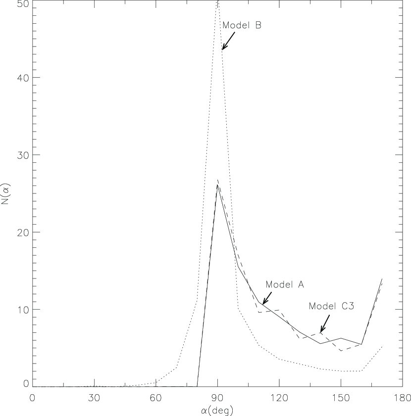
Figure 9: Distribution of the angle between polarization B-vectors and the filament axis, $\alpha$. Solid, dotted, and dashed lines represent, respectively, Models A, B, and C3. The $x$- and $y$-axes indicate $\alpha$ (deg) and the angle distribution $N(\alpha)$ in arbitrary unit. This shows that the angle $\alpha$ is concentrated to $\alpha\simeq 90^{\circ}$ in Model B, which has a high central density. Also in Models A and C3, the angle $\alpha$ is concentrated around $\alpha\simeq 90^{\circ}$. However, the distributions are more uniform compared with Model B, and have second peaks around $\simeq 180^{\circ}$.

As for the Serpens South Cloud, the magnetic field seems running perpendicular to the long axis of the molecular cloud (Sugitani et al., 2011), that is $\varphi\sim 90^{\circ}$. Using multi-line observations, Kirk et al. (2013) estimated the accretion rate onto an embedded cluster-forming region in this cloud: $\sim 30\,M_{\odot}\,{\rm yr^{-1}}$ is accreting along the axis of the filament while $\sim 130\,M_{\odot}\,{\rm yr^{-1}}$ is radially contracting (see also Figure 9 of André et al. (2014)). This large accretion rate is consistent with the fact that the observed mass per unit length (line-mass) $\lambda\sim 60\,M_{\odot}\,{\rm pc^{-1}}$ (Kirk et al., 2013) exceeds the critical line-mass of thermally supported filaments at 10K, $\lambda_{\rm th\ crit}\simeq 16.7\,M_{\odot}\,{\rm pc^{-1}}$ (Stodółkiewicz, 1963; Ostriker, 1964; Inutsuka & Miyama, 1997). The magnetically critical line-mass of the isothermal filaments that are perpendicularly threaded by the interstellar magnetic field is studied by Tomisaka (2014; hereafter paper I) under magnetohydrostatic conditions. This shows that the magnetic field can support the filament against the self-gravity, as long as the line-mass of the filament is $\lesssim 0.24\Phi_{\rm cl}/G^{1/2}$, where $\Phi_{\rm cl}$ and $G$ represent one half of the magnetic flux threading the filament per unit length and the gravitational constant, while the line mass is limited below $\lambda_{\rm th\ crit}=2\,c_{s}^{2}/G$ for a filament with no magnetic field ($c_{s}$ represents the isothermal sound speed). Since the magnetically critical line-mass is given $\lambda_{\rm mag\ crit}\simeq 22.4\,M_{\odot}\,{\rm pc^{-1}}(R_{0}/0.5{\rm pc})(B_{0}/10\mu{\rm G})$ (equation (39) of paper I), where the radius of the filament $R_{0}$ and the field strength $B_{0}$ give the amount of magnetic flux threading the filament, the filament of the Serpens South Cloud may be magnetically supercritical, $\lambda>\lambda_{\rm mag\ crit}$ not only thermally supercritical, $\lambda>\lambda_{\rm th\ crit}$. That is, when the magnetic flux per unit length is sufficiently large, such as $\Phi_{\rm cl}\gtrsim 3\,{\rm pc\,\mu G}\,(c_{s}/190\,{\rm m\,s^{-1}})^{2}$, the magnetic field plays a crucial role to support the filament.

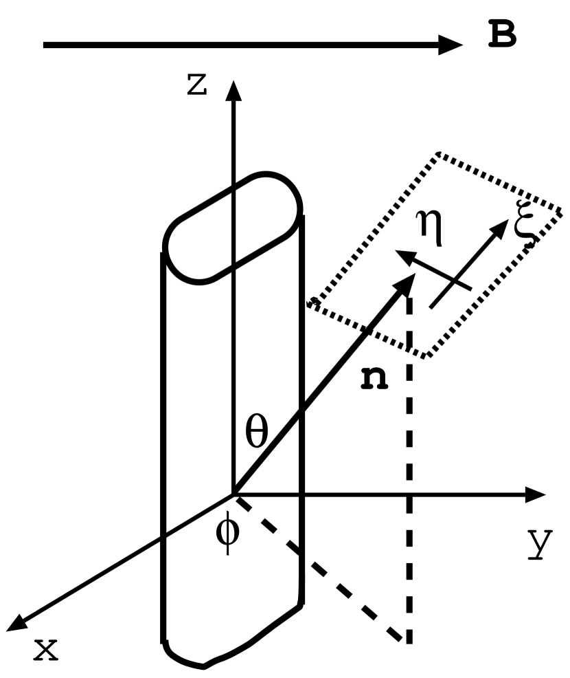
Figure 1: Schematic view of the geometry. Magnetohydrostatic filament extending in the $z$-direction is threaded by a magnetic field that runs globally in the $y$-direction. The filament is symmetric with respect to both the $x=0$ and $y=0$ planes. The observation line-of-sight is directed along a unit vector n, of which the direction is specified by two angles, $\theta$ and $\phi$. The observation is drawn on another plane with the coordinate $(\xi,\eta)$, of which the direction is defined in Equations (1a) and (1b). The filament is uniform in $z$-direction; therefore, the result is dependent only on $\xi$.

The relationship between magnetic field and the direction of the major axis of filaments is believed to be related to formation mechanisms. There are several mechanisms to form filamentary clouds. Nagai, Inutsuka, & Miyama (1998) considered an isothermal sheet with uniform magnetic fields and its fragmentation to filaments. They obtained filaments perpendicular to the magnetic field. When clouds contract along the magnetic field lines by the self-gravity, major axes of the filaments tend to align in the perpendicular direction to the magnetic field (e.g. Nakamura, & Li, 2008). Several models of MHD turbulence are proposed to form filamentary structures (Padoan et al., 2014). Sub-Alfvénic anisotropic turbulence leads to filaments to be aligned along the magnetic field lines (Stone, Ostriker, & Gammie, 1998). On the other hand, in super-Alfvénic turbulence, shocks form thin sheets (Padoan et al., 2001). Magnetic fields are also compressed in the sheets and as a result the field direction is parallel to the filamentary feature which comes from the compressed sheet. Inoue & Fukui (2013) considered collisions between two magnetized molecular clouds. The deformed MHD shock wave kinks the stream lines, and accumulates molecular gas into a filament extending perpendicular to the magnetic field (see their Figure 1). However, to discuss the formation mechanism, we have to reconstruct three-dimensional configuration of magnetic fields and filaments from two-dimensional polarization maps.

The degree of polarization is low if the object is observed from the direction parallel to the magnetic field, either for interstellar polarization due to the dichroic extinction in the optical and infrared wavelengths, or for the polarization of thermal emissions from dust grains aligned with the magnetic field. If the magnetic field is threading the filament perpendicularly, then an appreciable number of such objects must be observed as weakly polarized objects. However, observed examples of filaments indicate that the magnetic field is perpendicular to the filament. The polarization is affected by integration along the line-of-sight; therefore, it is not so simple to estimate the polarization pattern only from the angle between the local magnetic field and the line-of-sight. Thus, we calculate the expected polarization for such filaments and discuss the structure of the magnetohydrostatic filaments, especially, their magnetic structure expected in the polarization pattern.

The structure of this paper is as follows. Models of magnetohydrostatic filaments are taken from paper I. The models and formulation to calculate polarization are shown in $\S$2. In $\S$3, the expected polarization is given for two typical filament models; one with a relatively low center-to-surface density ratio, $\rho_{c}/\rho_{s}=10$, and another with a relatively high ratio, $\rho_{c}/\rho_{s}=300$. These two models exhibit distinctly different polarization patterns. Section 4 is devoted to discussion and exploration of the structures of filaments with different mass loadings (mass distribution against magnetic flux tube). In $\S$4, expected distributions of $\varphi$ are also calculated for magnetohydrostatic filamentary clouds.

2 Method

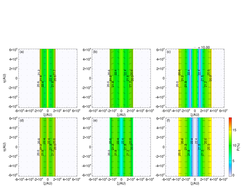
Figure 5: As for Figure 3 but for the $R_{0}=2\,c_{s}/(4\pi G\rho_{s})^{1/2}$, $\beta_{0}=1$, and $\rho_{c}=300\rho_{s}$ model (Model B).

Here, we focus on the polarization expected in the thermal dust emissions. Assuming an infinitely long filament, the magnetohydrostatic structure is specified with three nondimensional parameters (paper I): the center-to-surface density ratio, $\rho_{c}/\rho_{s}$, the plasma beta of the ambient material from far outside the cloud, $\beta_{0}\equiv\rho_{s}c_{s}^{2}/(B_{0}^{2}/8\pi)$, and the radius of a ‘parent’ filament normalized with the scale-height, $R_{0}/[c_{s}/(4\pi G\rho_{s})^{1/2}]\equiv R_{0}^{\prime}$, where the parent filament is a virtual state from which the filament is formed under magnetic flux freezing. We assume no additional turbulence motion in the filament. In these definitions, $\rho_{s}$ represents the density at the surface of the filament, outside of which a tenuous medium with a pressure of $\rho_{s}c_{s}^{2}$ is distributed, where $c_{s}$ and $G$ indicate the isothermal sound speed and gravitational constant, respectively. Beside these three scalar parameters, to specify a solution for magnetohydrostatic equilibrium, the distribution of magnetic flux against mass, which has a freedom of function, must be constrained. In paper I, we assumed a magnetic flux distribution which is realized when a uniform-density cylinder with a radius $R_{0}$ is threaded with a uniform magnetic field, $B_{0}$. The Cartesian coordinate system is used, where the filament is extending in the $z$-direction and the global magnetic field is running in the $y$-direction (see Figure 1 of paper I). The density distribution $\rho$, and magnetic field lines for equilibrium structures in the $x$-$y$ plane are shown in Figures 2, 5, and 7 of paper I. The density $\rho(x,y)$, and magnetic field ${\bf B}(x,y)=(B_{x}(x,y),B_{y}(x,y))$, are uniform in the $z$-direction and are dependent only on $(x,y)$.

When an object is observed along a line-of-sight whose direction is specified by a unit vector ${\bf n}$, another Cartesian coordinate is introduced to indicate the observation, $(\xi,\eta)$, of which the unit vectors are as follows:

$${\bf e}_{\eta} = \frac{{\bf e}_{z}-({\bf e}_{z}\cdot{\bf n}){\bf n}}{|{\bf e}_{z}-({\bf e}_{z}\cdot{\bf n}){\bf n}|},$$ (1a)

$${\bf e}_{\xi} = {\bf e}_{\eta}\times{\bf n},$$ (1b)

where the above definitions are the same as those given in Tomisaka (2011). The geometry of the filament and the direction of observation are shown in Figure 1. The polarization of the thermal dust emissions is calculated from the relative Stokes parameters (Lee & Draine, 1985; Fiege & Pudritz, 2000; Matsumoto, Nakazato, & Tomisaka, 2006; Tomisaka, 2011; Padovani et al., 2012):

$$q = \int\rho\cos 2\psi\cos^{2}\gamma ds,$$ (2a)

$$u = \int\rho\sin 2\psi\cos^{2}\gamma ds,$$ (2b)

where the integration is performed along the line-of-sight, $\rho$ is the density, and $\gamma$ and $\psi$ represent the angle between the magnetic field and the celestial plane, and the angle between the $\eta$-axis and the magnetic field projected on the celestial plane, respectively (see Figure 3 of Tomisaka (2011)). The E-vector distribution obtained from the polarimetry of background stars in the optical/near infrared regions appears similar to the polarization B-vector expected for the thermal dust emissions obtained here, except when the optical depth is thick. The dust temperature and the degree of dust alignment with the magnetic field may change spatially. However, in the present calculation, we assume that the dust temperature and the degree of alignment are spatially uniform. Observation of the filament from the direction of the magnetic field yields $\gamma=90^{\circ}$ (the magnetic field is perpendicular to the celestial plane). This configuration contributes nothing to the relative Stokes parameters; therefore, the observed degree of polarization is low when observed from the magnetic direction. The polarization direction $\chi$, is calculated from the relative Stokes parameters, $q$ and $u$ of Equations (2a) and (2b) as

$$\cos 2\chi = \frac{q}{(q^{2}+u^{2})^{1/2}},$$ (3a)

$$\sin 2\chi = \frac{u}{(q^{2}+u^{2})^{1/2}},$$ (3b)

which gives the vector for the degree of polarization,

$${\bf P}=\left(\begin{array}[]{c}P_{\xi}\\ P_{\eta}\end{array}\right)=\left(\begin{array}[]{c}P\sin\chi\\ P\cos\chi\end{array}\right).$$ (4)

The polarization degree $P$ is calculated relatively empirically:

$$P=p_{0}\frac{(q^{2}+u^{2})^{1/2}}{\Sigma-p_{0}\Sigma_{2}},$$ (5)

with use of the following integrated quantities:

$$\Sigma = \int\rho\ ds,$$ (6)

$$\Sigma_{2} = \int\rho\left(\frac{\cos^{2}\gamma}{2}-\frac{1}{3}\right)ds.$$ (7)

The parameter $p_{0}$ controls the maximum degree of polarization and we assume $p_{0}=0.15$ to fit the highest degree of polarization observed for the interstellar cloud.

The path length $\Delta s$, crossing one grid cell along the line-of-sight (used in Equations (2a), (2b), (6), and (7)) is calculated from the two-dimensional path length in the $x$-$y$ plane $\Delta\ell$, as

$$\Delta s=\Delta\ell/\cos\theta,$$ (8)

where $\cos\theta$ represents the direction cosine of the line-of-sight to the $z$-direction. Equation (6) contains only $\rho(x,y)$ in the integrand, so that $\Sigma$ is proportional to $(\cos\theta)^{-1}$. Other integrands also contain $\gamma$ and $\psi$, which are dependent on the line-of-sight direction or $\theta$ and $\phi$, where the spherical coordinate $(\theta,\phi)$ is adopted to specify the direction of the line-of-sight. The polarization distributions expected for the respective models are calculated with different $\theta$ and $\phi$.

3 Results

Model	$R_{0}$	$\beta_{0}$	$\rho_{c}$	$\lambda_{0}$
A……	$2\,c_{s}/(4\pi G\rho_{s})^{1/2}$	1	$10\,\rho_{s}$	$1.71\,c_{s}^{2}/G$
B……	$2\,c_{s}/(4\pi G\rho_{s})^{1/2}$	1	$300\,\rho_{s}$	$2.26\,c_{s}^{2}/G$

Table 1: Model parameters of Figure 2. $R_{0}$, $\beta_{0}$, $\rho_{c}$, and $\lambda_{0}$ represent the radius of a ‘parent cloud’ from which the filament is formed under magnetic flux freezing, the plasma beta of the ambient material from far outside the cloud, the density at the center of the filament, and the mass per unit length of the filament, respectively.

We calculate the polarization pattern for filaments in magnetohydrostatic balance obtained in paper I, of which the structures are shown in Figure 2. Figures 2(a) and (b) show typical models with low density contrast $\rho_{c}/\rho_{s}=10$, and with high density contrast $\rho_{c}/\rho_{s}=300$, respectively. The respective line-masses of the filaments are equal to $\lambda_{0}=1.71c_{s}^{2}/G=22c_{s}^{2}/(4\pi G)$ and $\lambda_{0}=2.26c_{s}^{2}/G=28c_{s}^{2}/(4\pi G)$ (model parameters are summarized in Table 1). Figure 2 shows that magnetic field is relatively uniform in the solution with low $\rho_{c}/\rho_{s}$ (Model A), while the magnetic field lines are strongly squeezed near the equator ($y=0$), when $\rho_{c}/\rho_{s}$ is high (Model B). To show the polarization distribution, we assume $c_{s}=0.19{\rm km\,s^{-1}}$, $\rho_{s}=10^{3}{\rm H_{2}\,cm^{-3}}$, and thus the scale-height $c_{s}/(4\pi G\rho_{s})^{1/2}=3.1\times 10^{4}{\rm AU}$.

3.1 Model with Low Central Density

Figure 3 shows the polarization pattern expected for Model A of Figure 2(a) with low density contrast, $\rho_{c}/\rho_{s}=10$. In the present paper, we show the direction of the B-vector for the observed electromagnetic wave as the direction of polarization, which coincides with the direction of the interstellar magnetic field when the temperature, density and magnetic field are all uniform. Observation of the filament from near its axis ($\theta=30^{\circ}$: Figures 3(a)-(c)) indicates that the polarization direction is dependent on the azimuthal angle, $\phi$. When observing the filament from $(\theta,\phi)=(30^{\circ},0^{\circ})$, which is a direction in the $x-z$ plane (perpendicular to the global magnetic field), the polarization vector is perpendicular to the filament (Figure 3(a)). However, when observing from a direction in the $y-z$ plane, such as $(\theta,\phi)=(30^{\circ},90^{\circ})$, the polarization vector is parallel to the filament (Figure 3(c)). Between these two, the polarization vector is directed from the upper-left to the lower-right (Figure 3(b)). The degree of polarization decreases when we increase $\phi$ from $\phi=0^{\circ}$ to $\phi=90^{\circ}$. This is reasonable because observation of the target from the direction of the magnetic field induces a low degree of polarization.

This is clarified by a comparison of three models with $\theta=80^{\circ}$ (Figures 3(d)-(f)). The direction $(\theta,\phi)=(80^{\circ},0^{\circ})$ is almost perpendicular to the global magnetic field (Figure 3(d)), while $(80^{\circ},90^{\circ})$ is almost parallel to it (Figure 3(f)). Observation from $\theta\simeq 90^{\circ}$ shows that the polarization vector is perpendicular to the filament, even for $\phi=45^{\circ}$. In this configuration, the degree of polarization is extremely low, when the filament is observed from near the magnetic field direction (Figure 3(f)). Thus, in the models shown in Figure 3, the polarization pattern coincides with that expected for the models consisting of a uniform magnetic field and uniform-density dust distribution.

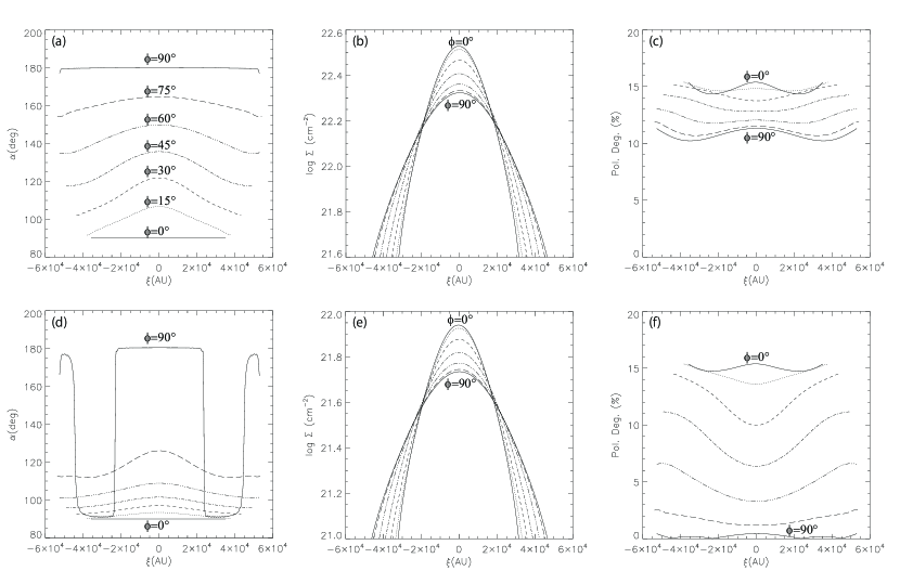
Figure 4: Expected polarization for the $R_{0}=2\,c_{s}/(4\pi G\rho_{s})^{1/2}$, $\beta_{0}=1$, and $\rho_{c}=10\rho_{s}$ model (Model A). Angle between the filament axis and polarization B-vector (left panels), column density (center panels), and degree of polarization (right panels) are plotted against the distance from the center of the filament. Upper and lower panels correspond to the models where the line-of-sight is selected with the angle from the filament axis at $\theta=30^{\circ}$ and $\theta=80^{\circ}$, respectively. Seven models with $\phi=0^{\circ}$ (solid line), $\phi=15^{\circ}$ (dotted line), $\phi=30^{\circ}$ (dashed line), $\phi=45^{\circ}$ (dash-dotted line), $\phi=60^{\circ}$ (two-dot chain line), $\phi=75^{\circ}$ (long dashed line), and $\phi=90^{\circ}$ (solid line) are shown.

Figure 4 shows the polarization angle (Figures 4(a) and (d)), the column density (Figures 4(b) and (e)), and the degree of polarization (Figures 4(c) and (f)) against the $\xi$-axis, which is taken to be perpendicular to the filament (see Figure 1). The upper and lower panels correspond to the cases of $\theta=30^{\circ}$ and $\theta=80^{\circ}$, respectively.

In Figures 4(a) and (d), $\alpha$, the angle between the filament axis and the polarization B vector are plotted. $\alpha=90^{\circ}$ indicates the polarization direction is perpendicular to the filament, while $\alpha=0^{\circ}$ and $\alpha=180^{\circ}$ indicate that the polarization direction and the filament are parallel. In Figure 4(a), the polarization angle increases from $\alpha\sim 90^{\circ}$ at $\phi=0^{\circ}$ (lower solid line; Figure 3(a)) to $\alpha\sim 180^{\circ}$ at $\phi=90^{\circ}$ (upper solid line; Figure 3(c)). As $\phi$ increases from $0^{\circ}$ to $90^{\circ}$, a deviation from the direction perpendicular to the filament appears first for the line-of-sight passing through the center, $\xi=0$. Figure 4(d) shows the models with $\theta=80^{\circ}$. The polarization angle $\alpha$ increases from $90^{\circ}$ to $180^{\circ}$ when changing the azimuth angle of the line-of-sight $\phi$, from $0^{\circ}$ to $90^{\circ}$, similar to that in Figure 4(a). Although the polarized intensity is weak for models with $\phi\gtrsim 60^{\circ}$ (Figure 4(f)), the polarization vector is within a $\pm 10^{\circ}$ deviation from the perpendicular direction (Figure 4(d)).

Figures 4(b) and (e) show the column density distribution for two groups with line-of-sights of $\theta=30^{\circ}$ and $80^{\circ}$, respectively. $\Sigma\propto(\cos\theta)^{-1}$; therefore, the column density distribution is scaled between two models of $\theta=30^{\circ}$ and $\theta=80^{\circ}$. This filament has a major axis in the $x$-axis (Figure 2), so that the width of $\Sigma$ distribution is observed to be narrower for the line-of-sight with $\phi=0^{\circ}$ and wider for $\phi=90^{\circ}$.

Figures 4(c) and (f) show the expected degree of polarization, $P$, which is dependent on $\theta$; when the filament is observed from the direction of the filament axis, a larger polarization intensity is expected (Figure 4(c)). For the line-of-sight of $\theta=30^{\circ}$, a relatively high degree of polarization, $10\%\lesssim P\lesssim 15\%$, is observed, irrespective of $\phi$. However, for the line-of-sight of $\theta=80^{\circ}$, although the polarization degree is as high as $P\sim 15\%$ for $\phi\lesssim 15^{\circ}$, the degree of polarization is suppressed to $P\lesssim 2\%$ for $\phi\gtrsim 75^{\circ}$. This is because the direction of $(\theta,\phi)=(90^{\circ},0^{\circ})$ is perpendicular to the global magnetic field, while that of $(\theta,\phi)=(90^{\circ},90^{\circ})$ is parallel to the global magnetic field. This is consistent with the expectation for a uniform-density filament threaded with a uniform magnetic field.

3.2 Model with High Central Density

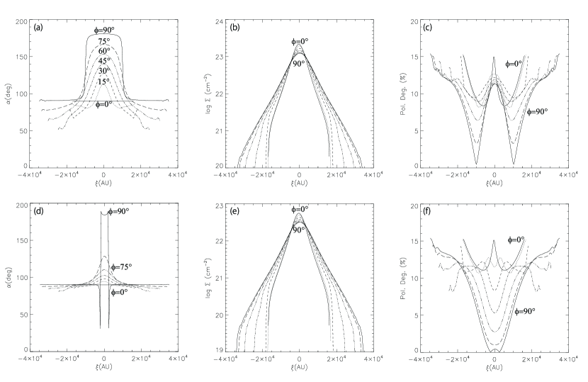
Figure 6: As for Figure 4 but for the $R_{0}=2\,c_{s}/(4\pi G\rho_{s})^{1/2}$, $\beta_{0}=1$, and $\rho_{c}=300\rho_{s}$ model (Model B).

Figures 5 and 6 show polarization patterns for Model B, which has the same parameter $R_{0}=2\,c_{s}/(4\pi G\rho_{s})^{1/2}$ and $\beta_{0}=1$ as that in the previous subsection, but with a different central density of $\rho_{c}=300\rho_{s}$. The upper panels of Figure 5 show the result for $\theta=30^{\circ}$. Figure 5(a) with $(\theta,\phi)=(30^{\circ},0^{\circ})$ shows that the polarization direction is perpendicular to the filament, which is similar to the model with low central density (Figure 3(a)). However, Figures 5(b: $\phi=45^{\circ}$) and (c: $\phi=90^{\circ}$) reveal a clear difference from the corresponding models with low central density (Figures 3 (b) and (c)). Figure 3 has polarization vectors running from upper-left to lower-right (b) and parallel to the filament (c). However, Figures 5 (b) and (c) have polarization vectors that are perpendicular to the filament, in a global sense. By increasing $\phi$ from $\phi=0^{\circ}$ to $\phi=90^{\circ}$, $\alpha$ increases from $\alpha\sim 90^{\circ}$ to $\alpha\sim 180^{\circ}$ for the inner central region of the filament $|\xi|\lesssim 1\times 10^{4}{\rm AU}$ (Figure 6(a)). In contrast, the outer part ($|\xi|\gtrsim 1\times 10^{4}{\rm AU}$) shows a different feature and $\alpha$ changes as $\alpha=90^{\circ}$ ($\phi=0^{\circ}$), $\alpha\sim 50-90^{\circ}$ ($\phi=45^{\circ}$), and $\alpha\sim 90^{\circ}$ ($\phi=90^{\circ}$). The outer part shows the polarization perpendicular to the filament ($\alpha\sim 90^{\circ}$).

Observation of the filament from the line-of-sight of $\theta=80^{\circ}$ reveals the polarization vector is also perpendicular to the filament (Figures 5(d)–(f)). Figure 6(d) shows that although the polarization direction angle $\alpha$ increases from $\alpha\simeq 90^{\circ}(\phi=0^{\circ})$ to $\alpha\simeq 180^{\circ}(\phi=90^{\circ})$ in the central part of the filament, $|\xi|\lesssim 5\times 10^{3}{\rm AU}$, $\alpha$ stays constant $\alpha\simeq 90^{\circ}$, irrespective of $\phi$ in the outer part of $|\xi|\gtrsim 5\times 10^{3}{\rm AU}$. Thus, Model B indicates a distinctly different polarization pattern from Model A, for both line-of-sights at $\theta=30^{\circ}$ and $\theta=80^{\circ}$.

The expected degree of polarization $P$ for Model B (Figures 6(c) and (f)) is also very different from that of Model A (Figures 4(c) and (f)). In Model A, $P$ decreases from 15% ($\phi=0^{\circ}$) to 0% ($\phi=90^{\circ}$), depending on $\phi$, in the case of $\theta=80^{\circ}$. This is also observed in the central part of the filament, $|\xi|\lesssim 2\times 10^{4}{\rm AU}$ in Model B. In contrast, for $|\xi|\gtrsim 2\times 10^{4}{\rm AU}$, $P\gtrsim 10\%$, irrespective of $\phi$ in Model B. Therefore, even if the line-of-sight is parallel to the global magnetic field, the outer part of the filament for Model B indicates strong polarization, in a direction perpendicular to the filament.

In summary, Model A and the inner part of Model B show similar polarization patterns. However, the polarization pattern is different for the outer part of the filament for Model B. The reason for this difference is clear. Magnetic field lines threading the filament of Model A are straight. In contrast, the magnetic field lines in the outer part of the filament of Model B are dragged inwardly near the equator, which induces a relatively strong $B_{x}$ component. Considering the line-of-sight at $(\theta,\phi)=(80^{\circ},90^{\circ})$, even when the filament is observed from the direction of the $y$-axis, the $B_{x}$ component, which is perpendicular to the line-of-sight, generates a certain amount of polarization.

4 Discussion

4.1 Effect of Mass Loading

Model	$R_{0}$	$\beta_{0}$	$\rho_{c}$	$\lambda_{0}$	${\cal N}$	$D({\cal N})$
C1……	$2\,c_{s}/(4\pi G\rho_{s})^{1/2}$	0.1	$19.2\rho_{s}$	$3c_{s}^{2}/G$	0.1	1.03028
C2……	$2\,c_{s}/(4\pi G\rho_{s})^{1/2}$	0.1	$30.54\rho_{s}$	$3c_{s}^{2}/G$	1	1.27324
C3……	$2\,c_{s}/(4\pi G\rho_{s})^{1/2}$	0.1	$416\rho_{s}$	$3c_{s}^{2}/G$	6	2.1875
C4……	$2\,c_{s}/(4\pi G\rho_{s})^{1/2}$	0.1	$416\rho_{s}$	$3.76c_{s}^{2}/G$	1	1.27324

Table 2: Model parameters for Figure 7. Same as Table 1, but where ${\cal N}$ and $D({\cal N})$ represent the mass concentration index defined in Equation (11) and the degree of mass concentration defined in Equation (13), respectively.

In this section, we compare the filaments with different mass loadings (mass distribution against magnetic flux). In paper I, we assume a mass loading that is realized when a uniform-density cylinder with a density $\rho_{0}$ and a radius $R_{0}$ is threaded by a uniform magnetic field $B_{0}$. In this model, the line-mass distribution $\lambda$, against the flux function $\Phi$, defined as the amount of magnetic flux counted from the central flux tube, is expressed as:

$${d\lambda\over d\Phi}=2\left(\rho_{0}\frac{R_{0}^{2}}{\Phi_{\rm cl}}\right)\left[1-(\Phi/\Phi_{\rm cl})^{2}\right]^{1/2},$$ (9)

where $\Phi_{\rm cl}$ is the magnetic flux per unit length of a cloud, which is defined as

$$\Phi_{\rm cl}=R_{0}B_{0},$$ (10)

and the flux function $\Phi$ varies from $-\Phi_{\rm cl}$ to $+\Phi_{\rm cl}$. This mass loading is extended to the following form:

$${d\lambda\over d\Phi}=2\left(\rho_{0}\frac{R_{0}^{2}}{\Phi_{\rm cl}}\right)\left[1-(\Phi/\Phi_{\rm cl})^{2}\right]^{{\cal N}/2}.$$ (11)

Here, ${\cal N}$ represents the degree of mass concentration to the central magnetic flux tube and we call ${\cal N}$ here as the mass concentration index. When ${\cal N}=0$, ${d\lambda/d\Phi}=$constant, irrespective of $\Phi$, which indicates a uniform mass loading:

$$\left.{d\lambda\over d\Phi}\right|_{\Phi=0}=\left.{d\lambda\over d\Phi}\right|_{\rm ave}\equiv\frac{\int_{-\Phi_{cl}}^{+\Phi_{cl}}{d\lambda\over d\Phi}d\Phi}{2\Phi_{cl}}.$$ (12)

By increasing the index ${\cal N}$, we are selecting the centrally concentrated mass loading and the degree of mass concentration

$$D({\cal N})\equiv\left.{d\lambda\over d\Phi}\right|_{\Phi=0}/\left.{d\lambda\over d\Phi}\right|_{\rm ave}=\frac{2\Gamma[({\cal N}+3)/2]}{\pi^{1/2}\Gamma[({\cal N}+2)/2]},$$ (13)

is an increasing function of ${\cal N}$, where $\Gamma$ represents the gamma function. This ratio $D({\cal N})$ is tabulated in Table 1 of Hanawa & Tomisaka (2014).

Figure 7 shows three models (Models C1-C3) with different ${\cal N}$, where the index ${\cal N}$ is chosen as ${\cal N}=0.1$ (Figure 7(a)), ${\cal N}=1$ (Figure 7(b)), and ${\cal N}=6$ (Figure 7(c)), respectively. However, the three models have the identical line-mass of $\lambda_{0}=3c_{s}^{2}/G$. The parameters for these models are summarized in Table 2. By increasing ${\cal N}$, the central density increases as $\rho_{c}=19.2\rho_{s}$ (Model C1), $\rho_{c}=30.54\rho_{s}$ (Model C2), and $\rho_{c}=416\rho_{s}$ (Model C3). See also Figure 5 of Hanawa & Tomisaka (2014). The gas is more concentrated toward the central magnetic flux tube; therefore, the gravity must be counter-balanced by the thermal pressure gradient, and thus the central density $\rho_{c}$ increases. Figure 7 shows that the area of the cross-cut is also contracted when a larger ${\cal N}$ is selected. The central concentration factor $D$, increases from $D=1.0303$ of ${\cal N}=0.1$ to $D=2.1875$ of ${\cal N}=6$.

In $\S$ 3, Figure 2 shows that Model B with high central density (Figure 2(b)) has magnetic field lines that are heavily squeezed toward the center near the equator ($y=0$), compared with Model A with a low central density (Figure 2(a)). However, Model C3 with a high central density shown in Figure 7(c) has a magnetic field structure similar to Models C1 and C2 with lower central densities (Figures 7(a) and (b)), especially for the outer part of the filament ($|x|\gtrsim 1$ in nondimensional distance). This is clearly shown by a comparison of Figures 7(c) and (d), both of which have the same central density $\rho_{c}=416\rho_{s}$ but a different mass-loading index ${\cal N}$ and line-mass $\lambda_{0}$ (for Model C3 of Figure 7(c), ${\cal N}=6$ and $\lambda_{0}=3c_{s}^{2}/G$ were selected, while for Model C4 in Figure 7(d), ${\cal N}=1$ and $\lambda_{0}=3.76c_{s}^{2}/G$ were selected). Although the magnetic field lines are dragged inwardly in both models, the field lines in Model C4 are squeezed toward the center more strongly than those of Model C3. Model C3 has a more centrally concentrated mass loading and the magnetic field is stored in the outer part of the filament. Thus, the magnetic field lines run relatively straight in this model. In conclusion, it is shown that the pattern of magnetic field lines is affected by how the mass is distributed against the magnetic flux (mass loading) and by the center-to-surface density ratio (or the line-mass $\lambda_{0}$). By increasing the mass concentration index ${\cal N}$, the magnetic field lines run more straight.

4.2 Does the Polarization Pattern Depend on Mass Loading?

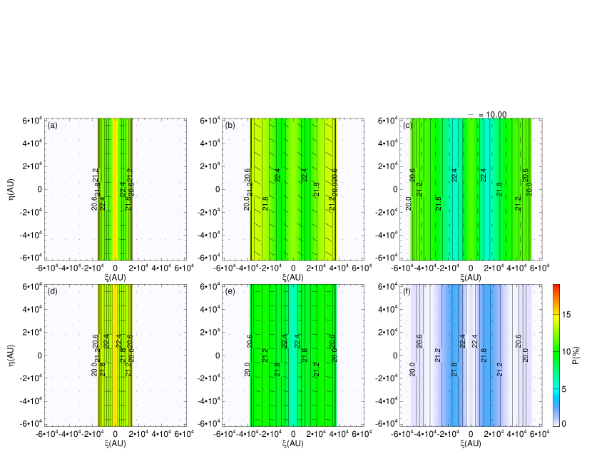
Figure 8: As for Figure 3 but for the $R_{0}=2\,c_{s}/(4\pi G\rho_{s})^{1/2}$, $\beta_{0}=0.1$, ${\cal N}=6$, and $\rho_{c}=416\rho_{s}$ model (Model C3).

As shown in $\S$4, the configuration of magnetic field lines is affected not only by the center-to-surface density ratio $\rho_{c}/\rho_{s}$ (paper I), but also by the mass-loading (or the mass-concentration index, ${\cal N}$). The expected polarization pattern is also affected by the mass-loading. Figure 8 shows the expected polarization pattern for Model C3 of Figure 7(c), which has a relatively large central density $\rho_{c}=416\rho_{s}$, but a large mass concentration index ${\cal N}=6$. Observation of the filament from a line-of-sight in the $x-z$ plane (perpendicular to the global magnetic field), such as $(\theta,\phi)=(30^{\circ},0^{\circ})$ (Figure 8(a)) and $(80^{\circ},0^{\circ})$ (Figure 8(d)), we observe the polarization vector to be perpendicular to the filament, which is similar to Figures 3(a) and (d) and Figures 5(a) and (d). The same polarization pattern is observed in the case of $(\theta,\phi)=(80^{\circ},45^{\circ})$ in all Figures 3, 5, and 8.

For lines-of-sight with $(\theta,\phi)=(30^{\circ},45^{\circ})$ (Figure 8(b)), the polarization vector is running from the upper-left to the lower-right, which is similar to Figure 3(b) but different from Figure 5(b). Figure 8(c), in which the polarization vector is parallel to the filament, does not resemble Figure 5(c) but does resemble Figure 3(c). Observation of the filament from almost the direction of global magnetic field, $(\theta,\phi)=(80^{\circ},90^{\circ})$ (f), reveals a low degree of polarization. This is not observed in Figure 5(f), but is evident in Figure 3(f). In summary, Model C3 has a polarization pattern similar to Model A (${\cal N}=1$ and low central density model), but not similar to Model B (${\cal N}=1$ and high central density model). This clearly shows that the models with a large mass concentration index ${\cal N}$ have straight magnetic field lines, even near the equator of the outer part. This gives a polarization pattern similar to Model A, but not similar to Model B, which indicates that the observed polarization pattern is affected not only by the center-to-surface density ratio $\rho_{c}/\rho_{s}$, but also by mass concentration index, ${\cal N}$. Even if the central density is high, as in Model C3, the magnetic field lines are relatively straight, which induces the polarization pattern expected for a filament threaded by a straight magnetic field.

4.3 Distribution of the Angles between Polarization Vector and the Filament Axis

The Planck polarization observation has indicated the distribution of angles between the polarization B-vector and the direction of iso-column density contours, $\varphi$ (Planck Collaboration Int. XXXV, 2015). Since the angle $\varphi$ corresponds to $\alpha$ of this paper, we calculate the distribution of angle $\alpha$. For each model, the number of grids whose angles equal to $\alpha$ is calculated. Since this number of grids also depends on the direction of line-of-sight or $\theta$ and $\phi$, we express this as $n(\alpha;\theta,\phi)$. If we assume the line-of-sight direction is randomly chosen, the expected distribution of $\alpha$ is obtained as follows:

$$N(\alpha)=\frac{\int_{\theta=0^{\circ}}^{\theta=90^{\circ}}\int_{\phi=0^{\circ}}^{\phi=180^{\circ}}n(\alpha;\theta,\phi)\sin\theta\,d\theta\,d\phi}{\int_{\theta=0^{\circ}}^{\theta=90^{\circ}}\int_{\phi=0^{\circ}}^{\phi=180^{\circ}}\sin\theta\,d\theta\,d\phi}.$$ (14)

In Figure 9, we plot $N(\alpha)$ for three models, Models A (Figure 3), B (Figure 5), and C3 (Figure 8). To obtain the expected distribution of angle $n(\alpha;\theta,\phi)$, we do not take into account of the polarization degree $P$ and the polarized intensity. However we only count the grids where the column density exceeds $10^{21}{\rm H_{2}\,cm^{-2}}$.

Figure 9 shows that all the three models have distribution function whose peaks are located around $\alpha\simeq 90^{\circ}$, which is consistent with the polarization observation with Planck seen in such as Taurus, Lupus, and Chamaeleon-Musca. Model B has a strongly concentrated distribution around $\alpha\simeq 90^{\circ}$, while Models A and C3 have more uniform distributions and have another peak around $\alpha\simeq 180^{\circ}$.

Figure 9 shows that even if the magnetic field is running perpendicular to the filament in three dimension, some clouds may be observed with $\alpha\simeq 0^{\circ}$ (filaments are aligned to the magnetic field). Thus, we should pay attention to the projection effect in reconstructing the three dimensional configuration of the filament.

5 Summary

We have identified two types of polarization patterns from mock observation of magnetohydrostatic filaments perpendicularly threaded by magnetic field. When the center-to-surface density ratio for the filament is small, a pattern is realized in which the B-vector is perpendicular to the filament, when the filament is observed from the line-of-sight perpendicular to the magnetic field. However, when the filament is observed from the direction of the magnetic field, the observed degree of polarization is expected to be very low. This pattern is similar to that expected for a filament with uniform density and uniform magnetic field. This is also expected for a filament with high central density, if the mass concentration index ${\cal N}$ is large (gas mass is concentrated toward the central magnetic flux tube), because the magnetic field lines are globally straight also in this case.

In contrast, another pattern is expected for a filament with both a high center-to-surface density ratio and a low mass concentration index ${\cal N}\sim 1$. In this pattern, the B-vector is observed perpendicular to the filament, even when the filament is observed from the direction of the magnetic field. This may explain why filaments are often associated with perpendicular magnetic field lines.

This work was supported in part by the Grant-in-Aid for Scientific Research (A) (No. 21244021) from the Japan Society for the Promotion of Science (JSPS), and by HPCI Strategic Program of the Japanese Ministry of Education, Culture, Sports, Science and Technology (MEXT). Numerical computations were conducted, in part, on Cray XT4 and Cray XC30 computers at the Center for Computational Astrophysics (CfCA) at the National Astronomical Observatory of Japan.

(a)                                                            (b)

Figure 2: Magnetohydrostatic structures of models with $R_{0}=2\,c_{s}/(4\pi G\rho_{s})^{1/2}$ and $\beta_{0}=1$. Two models are shown with different density contrasts between the center and the surface; (a) $\rho_{c}/\rho_{s}=10$ (Model A) and (b) $\rho_{c}/\rho_{s}=300$ (Model B), which are taken from Figures 5(a) and (c) of paper I. Closed solid lines represent the density contours, where the contour levels are selected as 1, 2, 3, 5, 10, 20, 30, 50, 100, and 200 $\times\rho_{s}$. Dashed lines running vertically represent the magnetic field lines, and the solid lines represent special magnetic field lines in contact with the cloud surface, $\rho=\rho_{s}$. The dotted circle is shown to indicate the radius of the non-magnetized filament with the identical density contrast. Model parameters shown in this figure are summarized in Table 1. The $x$- and $y$-axes represent the distance normalized with the scale-height $c_{s}/(4\pi G\rho_{s})^{1/2}$.

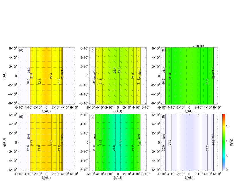
Figure 3: Expected polarization for the $R_{0}=2\,c_{s}/(4\pi G\rho_{s})^{1/2}$, $\beta_{0}=1$ and $\rho_{c}=10\rho_{s}$ model (Model A). Upper and lower panels correspond to models where the line-of-sight is selected with the angle from the filament axis at $\theta=30^{\circ}$ and $\theta=80^{\circ}$, respectively. Left, center, and right panels represent the cases of $\phi=0^{\circ}$, $45^{\circ}$, and $90^{\circ}$, respectively. Black bars represent the direction of the B-vector for the electromagnetic wave (polarization vector). False color represents the degree of polarization and black contour lines indicate the iso-column-density lines with a logarithmic step of $\Delta\log\Sigma=0.3$.

(a)                                                            (b)

                 (c)                                                            (d)

Figure 7: Structure of hydrostatic filaments with the same line-mass but different mass-loadings. Models C1 (a), C2 (b), and C3 (c) have identical line-mass of $\lambda_{0}=3c_{s}^{2}/G$. Parameters of each panel are (a) ${\cal N}=0.1$ and $\rho_{c}=19.2\rho_{s}$, (b) ${\cal N}=1$ and $\rho_{c}=30.54\rho_{s}$, and (c) ${\cal N}=6$ and $\rho_{c}=416\rho_{s}$. Model C4 in (d) has the same central density of $\rho_{c}=416\rho_{s}$ as Model C3 (c) but different ${\cal N}=1$, and thus line-mass $\lambda_{0}=3.76c_{s}^{2}/G$. Solid and dashed lines represent the density contours and magnetic field lines, respectively, as in Figure 2. Centrally concentrated mass-loading (increasing ${\cal N}$ from (a) to (c)) induces higher central density. The parameters for these models are given in Table 2.

References

- André et al. (2014) André, Ph., Francesco, J.D., Ward-Thompson, D., et al. 2014, in Protostars and Planets VI. ed. H. Beuther, R.S. Klessen, C.P. Dullemond, & T. Henning (Tucson: University of Arizona Press), 27
- Arzoumanian et al. (2011) Arzoumanian, D., André, Ph., Didelon, P., et al. 2011, A&A, 529, L6
- Barnett (1915) Barnett, S.J. 1915, Phys. Rev., 6, 239
- Clark, Peek, & Putman (2014) Clark, S. E., Peek, J. E. G., & Putman, M. E. 2014, ApJ, 789, 82
- Fiege & Pudritz (2000) Fiege, J. D., & Pudritz, R. E. 2000, ApJ, 544, 830
- Draine (2011) Draine, B.T. 2011, Physics of the Interstellar and Intergalactic Medium, (Princeton, Princeton University Press) Chap.26
- Draine, & Weingartner (1996) Draine, B.T., & Weingartner, J.C. 1996, ApJ, 470, 551
- Gaensler et al. (2011) Gaensler, B. M., Haverkorn, M., Burkhart, B., et al. 2011, Nature, 478, 214
- Hanawa & Tomisaka (2014) Hanawa, T., & Tomisaka, K. 2015, ApJ, 801, 11
- Hacar et al. (2013) Hacar, A., Tafalla, M., Kauffmann, J., & Kovács, A. 2013 A&A, 554, A55
- Hill et al. (2011) Hill, T., Motte, F., Didelon, P., et al. 2011, A&A, 533, A94
- Hoang, & Lazarian (2009) Hoang, T., & Lazarian, A. 2009, ApJ, 695, 1457
- Iacobelli et al. (2014) Iacobelli, M., Burkhart, B., Haverkorn, M., et al. 2014 A&A, 566, A5
- Inoue & Fukui (2013) Inoue, T., & Fukui, Y. 2013, ApJ, 774, L31
- Inutsuka & Miyama (1997) Inutsuka, S.-I., & Miyama, S.M. 1997, ApJ, 480, 681
- Kirk et al. (2013) Kirk, H., Myers, P.C., Bourke, T.L., et al. 2013, ApJ, 766, 115
- Koch, Tang & Ho (2013) Koch, P.M., Tang, Y.-W., & Ho, P.T.P. 2013, ApJ, 775, 77
- Lee & Draine (1985) Lee, H. M., & Draine, B. T. 1985, ApJ, 290, 211
- Li et al. (2013) Li, H.-b., Fang, M., Henning, T., & Kainulainen, J. 2013, MNRAS, 436, 3707
- Matsumoto, Nakazato, & Tomisaka (2006) Matsumoto, T., Nakazato, T., & Tomisaka, K. 2006, ApJ, 637, L105
- Menshchikov et al. (2010) Men’shchikov, A., André, Ph., Didelon, P., et al. 2010, A&A, 518, L103
- Miville-Deschênes et al. (2010) Miville-Deschênes, M.-A., Martin, P.G., Abergel, A., et al. 2010, A&A, 518, L104
- Nagai, Inutsuka, & Miyama (1998) Nagai, T., Inutsuka, S., & Miyama, S.M. 1998, ApJ, 506, 306
- Nakamura, & Li (2008) Nakamura, F., & Li, Z.-Y. 2008, ApJ, 687, 354
- Ostriker (1964) Ostriker, J.P., 1964, ApJ, 140, 1056
- Padoan et al. (2014) Padoan, P., Federrath, C., Chabrier, G., et al. 2014, in Protostars and Planets VI. ed. H. Beuther, R.S. Klessen, C.P. Dullemond, & T. Henning (Tucson: University of Arizona Press), 77
- Padoan et al. (2001) Padoan, P., Juvela, M., Goodman, A.A., & Nordlund, Å. 2001, ApJ, 553, 227
- Padovani et al. (2012) Padovani, M., Brinch, C., Girart, J.M., et al. 2012, A&A, 543, A16
- Palmeirim et al. (2013) Palmeirim, P., André, Ph., Kirk, J. et al. 2013, A&A, 550, A38
- Planck Collaboration Int. XXXV (2015) Planck Collaboration Int. XXXV, 2015, submitted to A&A(arXiv:1502.04123)
- Purcell (1979) Purcell, E.M. 1979, ApJ, 231,404
- Schneider et al. (2012) Schneider, N., Csengeri, T., Hennemann, M., et al. 2012, A&A, 540, L11
- Stodółkiewicz (1963) Stodółkiewicz, J.S., 1963, Acta Astr., 13, 30
- Stone, Ostriker, & Gammie (1998) Stone, J.M., Ostriker, E.C., & Gammie, C.F. 1998, ApJ, 508, L99
- Sugitani et al. (2011) Sugitani, K., Nakamura, F., Watanabe, M., et al. 2011, ApJ, 734, 63
- Tomisaka (2011) Tomisaka, K. 2012, PASJ, 63, 147 (erratum, PASJ, 63, 715)
- Tomisaka (2014) Tomisaka, K. 2014, ApJ, 785, 24 (paper I)
(a) (b)
(a) (b)
(c) (d)