A Homotopy Method for Large-Scale Multi-Objective Optimization

Abstract.

A homotopy method for multi-objective optimization that produces uniformly sampled Pareto fronts by construction is presented. While the algorithm is general, of particular interest is application to simulation-based engineering optimization problems where economy of function evaluations, smoothness of result, and time-to-solution are critical. The presented algorithm achieves an order of magnitude improvement over other geometrically motivated methods, like Normal Boundary Intersection and Normal Constraint, with respect to solution evenness for similar computational expense. Furthermore, the resulting uniformity of solutions extends even to more difficult problems, such as those appearing in common Evolutionary Algorithm test cases.

1. Introduction

The problem of scalar function minimization is ubiquitous in modern engineering sciences and a number of algorithms exist that exploit various functional characteristics to reach timely solutions. Far more difficult is the problem of vector function minimization, where a of number different, often conflicting, objectives are optimized in such a way as to strike a balance that pleases the end-user. The presence of multiple output dimensions requires a generalization of our concept of optimality, demands significantly more computational effort, as well as compounds the inherent difficulty of the problem.

1.1. Problem Statement

Precisely stated, and adopting the notation of [11], we seek to address the problem

(1) $$\min_{\textbf{x}\in D}\textbf{F}(\textbf{x}) = [F_{1}(\textbf{x}),F_{2}(\textbf{x}),...,F_{k}(\textbf{x})]^{T}$$

subject to

$$g_{j}(\textbf{x}) \leq 0 \forall j\in[1,m]$$

$$h_{l}(\textbf{x}) =0 \forall l\in[1,e]$$

where the objective functions, $F_{i}$, are bounded and defined over the set $D\in\mathbb{R}^{n}$. Here, x is a vector of independent design variables of length $n$ and contained in $D$. In this formulation, the set of objective functions, $\left\{F_{i}(\textbf{x})\colon\forall i\in[1,k]\right\}$, form a map

(2) $$\textbf{F}\colon\mathbb{R}^{n}\to\mathbb{R}^{k}$$

from design space to objective space. The set of all $\textbf{x}\in D$ satisfying the inequality constraints, $g_{j}(\textbf{x})\leq 0$, and the equality constraints, $h_{l}(\textbf{x})=0$,

(3) $$X\colon=\left\{\textbf{x}\in D\colon\begin{matrix}g_{j}(\textbf{x})\leq 0&\forall j\in[1,m]\\ h_{l}(\textbf{x})=0&\forall l\in[1,e]\end{matrix}\right\}$$

is called the feasible set. It’s image in objective space

(4) $$Z\colon=\left\{\textbf{F}(\textbf{x})\colon\textbf{x}\in X\right\}$$

is denoted the attainable set.

In the general case, the $\textbf{F}_{i}$ functions can not be simultaneously optimized and compromise solutions must be considered. Therefore, our goal is to discover locally Pareto optimal points, which are solutions that can not be improved in all objectives simultaneously when compared to its neighbors in the feasible set. The set of all Pareto optimal points (when viewed in objective space) is called the Pareto front and explicitly maps the optimal values that can be attained when considering conflicting objectives.

In this paper we propose a method for computing high-quality discrete approximations of Pareto fronts. We begin by reviewing existing methods and commenting on their ammenability to large problems with many objectives. We then review previous work on a particular homotopy method and demonstrate an alternative formulation. After explicitly generalizing this approach to problems arbitary dimension, we compare our formulation to methods using three test problems from the literature. Finally, we present an application of this method to a problem in the field of particle accelerator design and discuss performance related to various benchmarks. We conclude by mentioning futher improvements and future research directions.

2. Related Work

As a result of the ubiquity of problems that fit the formulation given in (1), a variety of methods have been devised for sampling high-dimensional Pareto fronts.

2.1. Scalarization

One simple method involves explicitly imposing an order on the objective space. This can be done, for example, by introducing a suitable scalarization function projecting the objective space onto, and using the well-ordered property of, the real numbers to define a solution. This effectively reduces the task of (1) to a scalar minimization problem amenable to solution via an number of established numerical optimization techniques.

(5) $$\begin{matrix}\min_{\textbf{x}\in X}s(\textbf{F}(\textbf{x});\boldsymbol{\lambda})\mbox{ with }s(\textbf{F};\boldsymbol{\lambda})\colon\mathbb{R}^{k}\to\mathbb{R}\end{matrix}$$

While the approach is straightforward, the mapping between the scalarization parameters ($\boldsymbol{\lambda}$) and corresponding solution’s location on the Pareto front generally is not, and fronts generated by blindly probing the $\boldsymbol{\lambda}$-space often suffer from highly irregular sampling [11].

2.2. Evolutionary Algorithms

Rather than attempting to break the overall sampling task into a series of subproblems, as in the proposed scalarization approach, population-based methods, generally speaking, attempt to solve the problem as a whole. This is done, typically, by generating sets of mutually non-dominated solutions using Evolutionary Algorithms (EAs). A number of specific heuristics have been proposed (see [20], [11], [2], and [16]) using a variety of techniques to balance the discovery of non-dominated solutions with diversity criteria to discourage solution crowding.

While EAs are capable of performing well on even the most difficult problems, some key aspects suggest that they are not ideal for all objective types. First, as in [2], solutions are evaluated based on their relative dominance to other solutions in the population. Unlike scalarization methods that provide some necessary or sufficient conditions for optimality of solutions, this does not actually guarantee Pareto optimality of the resulting solution candidates. Additionally, the nature of the non-dominating fitness criteria inherently limits the scalability of this class of algorithms as it involves comparing elements of the population against each other, naturally implying some super-linear running time behavior with increasing population size [2, 8]. While parallelizing the evaluation step [5] or distributing various objective space regions to different processors [4] can partially mitigate this effect, population size must still increase exponentially with objective space dimension to maintain an evenly sampled Pareto front. Furthermore, increasing the number of objectives distorts the utility of the dominance ranking criterion as the hypersurface-area to hypervolume effect permits a higher proportion of non-dominated solutions and weakens selection pressure [7].

2.3. Geometric Methods

Rather than rely on a flood of function evaluations to explore the solution space, a final class of methods uses the scalarization approach, but exploits geometrical arguments to further restrict the attainable set for each optimization subproblem. Practically, this is accomplished by adding auxiliary constraint functions to steer the scalar optimization subroutines towards desirable solutions and deliver an evenly sampled front. The Normal Boundary Intersection (NBI) [1] and the Normal Constraint (NC) [12] method essentially restrict each optimization subproblem to consider only solutions that lie on the normal vector emanating from the convex hull of the individual minimizers (CHIM).

These methods make intuitive sense, as well as produce well sampled fronts. However, by restricting the attainable set to the CHIM normal, these approaches are only capable of capturing Pareto points that lie within the projection of this hull. Furthermore, these points are only equally distributed when viewed from the CHIM frame, as seen in figure 1.

Figure 1. In the NBI and NC methods, evenly spaced points on the CHIM are projected to the Pareto front. Unfortunately, as a result of the front geometry, the resulting sample points are not always evenly spaced. The fact that $d_{1}\neq d_{2}$ illustrates this effect.

The specific algorithms also exhibit some scalability bottlenecks, especially when increasing the number of objectives, $k$. Since the boundaries of the Pareto front are not know a priori, it is often difficult to decide where to place solution points on the CHIM. In [13] and [14], it is suggested to divide the solution algorithm into two phases; the first samples the trade-offs between all combinations of individual objectives to establish the boundaries of the complete front. The second phase involves solving a set of scalar optimization subproblems to find Pareto optimal points on the interior of this boundary. The first phase, consists of $\sum_{i=2}^{k-1}\binom{k-1}{i}$ “sub-fronts” to sample before the domain is properly bounded and sampling on the interior can begin. Furthermore, the recursive nature of sub-front sampling, such as this, limits the scalability to only $i$ parallel sub-front’s per step of the initial phase.

3. Motivating Example

Consider a standard bi-objective minimization problem.

(6) $$\min_{\textbf{x}\in X}\textbf{F}(\textbf{x})=[F_{1}(\textbf{x}),F_{2}(\textbf{x})]^{T}$$

A straightforward method for constructing a well-sampled discrete Pareto front representation, as discussed in [17] and [18], involves scalarizing the objectives and adding explicit solution spacing terms to the equality constraint set.

Using a simple weighted sum scalarization, we obtain the following scalar objective function,

(7) $$f(\textbf{x},\lambda)=(1-\lambda)F_{1}(\textbf{x})+\lambda F_{2}(\textbf{x})\mbox{ with }\begin{array}[]{rcl}0\leq\lambda\leq 1\end{array}$$

the minimizer of which, $\min_{\textbf{x}\in X}f(x,\lambda)=\textbf{f}(\lambda)$, is a parametric expression of the Pareto front. The endpoints, $\textbf{f}(0)$ and $\textbf{f}(1)$ correspond to the minima of the individual objective functions, $F_{1}(\textbf{x})$ and $F_{2}(\textbf{x})$, respectively, while the parameter $\lambda$ controls the transition between these extremes.

The mapping between $\lambda$ and position along the Pareto front is often highly nonlinear. However, as presented in [18], we can exploit this additional degree of freedom to sample specific points along the curve by treating the $\lambda$ parameter as a design variable. This added flexibility is complemented by an auxilary equality constraint, typically of the form

(8) $$||\textbf{F}(\textbf{x})-\textbf{F}_{prev}||^{2}=\gamma^{2}$$

that explicitly enforces equal spacing between adjacent sample points. This allows a suitable scalar optimization procedure to minimize the scalarized objective function (7) subject to the constraint that the result lies a certain distance, $\gamma$, from a specified point, $\textbf{F}_{prev}$. By seeding this procedure with either of the objective minima, for instance with $\textbf{F}(\textbf{x}_{0})=\textbf{f}(0)$, we can iteratively generate evenly spaced samples by “marching” along the Pareto front carrying out the following scalarized minimization

(9) $$\min\limits_{\textbf{x}_{p}\in X} (1-\lambda_{p})F_{1}(\textbf{x}_{p})+\lambda_{p}F_{2}(\textbf{x}_{p})\text{ with }0\leq\lambda_{n}\leq 1$$

(10) subject to

$$||\textbf{F}(\textbf{x}_{p})-\textbf{F}(\textbf{x}_{p-1})||^{2}=\gamma^{2}$$

for $p$ up to the number of desired sample points, $P$ (provided a suitable step-size, $\gamma$).

While this method produces well-sampled Pareto front representations, even for difficult problems, it requires sequential variation of the $\lambda$-parameter and serial computation of the sample point locations, thereby limiting its scalability and application to large problems and those with expensive objective functions.

The authors address this concern in [18] by extending the algorithm to parallel processing environments. This is done, primarily, by replacing references to previously computed sample points, $\textbf{F}(\textbf{x}_{p-1})$, with continually updated position estimates, $\textbf{F}(\textbf{x}_{p-1}^{current})$. This way, we create a set of semi-independent and simultaneously solvable scalar optimization sub-problems, coupled only through the auxilary equispacing constraint (8). In fact, we can distribute the subproblems to as many processors as we have Pareto front sample points, thereby lifting the scalability limits imposed by the sequential algorithm. This iterative refinement, of course, requires defining a set of initial estimates, $\{\textbf{F}_{p}\for p\in[1,P]\}$, that form an ansatz front; however, this can be as simple as a set of equally spaced points on the line connecting the objective space images of the individual function minimizers.

One concern with enforcing an explicit spacing constraint like (10) is that, without additional information about the arc-length of the true Pareto front, a suitable step-size parameter, $\gamma$, can not be established a priori. One can imagine a bootstrapping process whereby the total arc-length of the front is estimated and refined by successive applications of the algorithm; however, this would involve serial repetitions of the front sampling procedure, limiting parallel scalability.

A simpler approach that accomplishes the same goal is to adjust constraint (10) to, instead, explicitly enforce equal spacing between a point’s up- and down-stream neighbors. Specifically, a modified constraint of the form

(11) $$||\textbf{F}_{p}-\textbf{F}_{p+1}||^{2}-||\textbf{F}_{p}-\textbf{F}_{p-1}||^{2}=0$$

eliminates the need to estimate the Pareto front arc-length a priori by not fixing the spacing between points and allowing the front representation to expand indefinitely.

Figure 2. The solid circle in the plot on the left represents the feasible region permitted by constraint (10) for ansatz node $A$, given unity $\alpha$, while the solid line on the right represents the feasible region implied by constraint (11) for ansatz node $B$.

Rephrasing the constraint this way, however, has other important ramifications, as well. First, it ameliorates an unfortunate consequence of the formulation in (10) that limits the optimizer’s improvement per iteration to $\gamma$. Because of this limited step size, if the ansatz is sufficiently distant from the real Pareto optimal front, applying the method of [18] will require multiple iterations to generate a set of truly optimal solutions. Constraint (11), however, is more in line with NBI and NC methods (described above) that do not restrict step sizes, allowing the sample points to converge to the Pareto front more quickly.

Most importantly, by eliminating explicit references to the total arc-length, only local communication of current $\textbf{F}_{p}$ values between adjacent optimization sub-problems is required. This means we can concurrently compute uniformly distributed Pareto front representations using only local, asynchronous communication between neighboring compute nodes, a key feature of massively scalable algorithms. In fact, the amount of parallelism is bounded only by the number of Pareto front sample points required, $P$, which (to obtain a truly uniformly spaced representation) often scales exponentially with the number of objectives.

4. Multi-Dimensional Generalization

Generalizing this approach to multiple objectives requires not only auxiliary scalarization variables, but a full generalization of the ansatz concept and corresponding constraints as well. The equidistance constraint naturally applies in the context of the bi-objective linear ansatz. In fact, during the first iteration, it reduces the attainable set in a manner that is functionally equivalent to the constraints used in the NBI and NC methods. Similarly confining the attainable set as the dimension of the problem increases is accomplished by properly balancing the positions of neighboring ansatz nodes in $k$-space. In addition to establishing this neighbor-wise balance, we identified a number of further requirements for any meshing solution:

1. An ansatz mesh must have an approximately equal distribution of points over its $k-1$ area.

2. It should easily support a range of sampling resolutions.

3. It should scale with problem dimension.

4. It should support distributed generation with low computational, as well as storage, overhead.

To address these requirements, we supply an ansatz with the simplicity and scalability of a rectilinear, coordinate-parallel mesh that resides on the convex hull of the individual objective minimizers. Since we deal in a normalized objective space, we can generate the initial front sample points by intersecting a rectilinear grid with the unit $k-1$ simplex. We then establish equidistance constraint relationships (or adjacency pairs) along the coordinate-parallel mesh axes. For instance, the scalarized sub-problem at point C will be augmented with two additional constraints, (12) and (13), both of which are based on (11). As in the two objective problem discussed above, this initially reduces the attainable set of this optimization subproblem to the simplex normal.

(12) $$||\textbf{F}_{C}-\textbf{F}_{A}||^{2}-||\textbf{F}_{C}-\textbf{F}_{E}||^{2}=0$$

(13) $$||\textbf{F}_{C}-\textbf{F}_{B}||^{2}-||\textbf{F}_{C}-\textbf{F}_{D}||^{2}=0$$

The scalarized subproblem at point D, however, will only be augmented with a single additional constraint, (14). This is because point D actually lies on the Pareto front of the bi-objective subproblem in the $f_{1}\times f_{2}$ plane and needs no further restriction of the attainable set.

(14) $$||\textbf{F}_{D}-\textbf{F}_{A}||^{2}-||\textbf{F}_{D}-\textbf{F}_{1}^{*}||^{2}=0$$

The ansatz is completed by reprojecting the result into $k$-space resulting in a uniformly-distributed linear interpolation between the $k$ individual objective minimizers and preserving the coordinate-wise equal spacing between the constituent points. This process is illustrated for a three objective problem in figure 3 with the final result projected back into 3-space in figure 4.

Figure 3. On the left, we generate the ansatz points by intersecting a rectilinear grid with the convex hull of the individual minimizers, denoted by the shaded region (a $k-1$ simplex). We establish neighbor-relations on the right using coordinate-parallel axes.

Figure 4. The full ansatz for a three objective problem as seen in the $f_{1}\times f_{2}\times f_{3}$ space.

This ansatz concept addresses requirements I and II by creating a uniform tensor-product mesh and supporting a range of axis-wise sampling densities. In this way, we avoid uneven sampling of the Pareto front and allow the user to explicitly specify the level of detail required.

Moreover, the coordinate-parallel nature of this solution addresses characteristic III by adding only two more mesh point neighbors per additional dimension of the ansatz. In other words, the degree of each node in the graph is bounded by $2(k-1)$ while adequately reducing the attainable set. Ultimately, this means that the number of additional constraints added to the overarching optimization problem to ensure equispacing of the Pareto front, as well as the magnitude of the data dependency of the optimization sub-problem occurring at each mesh node, scales linearly with the number of target objectives.

Figure 5. A similarly constructed ansatz for a four objective problem, projected onto the $f_{1}\times f_{2}\times f_{3}$ subspace.

Finally, since all of the coordinate transforms and neighbor-discovering operations can be accomplished independently for each point, this meshing strategy supports fully distributed generation, satisfying requirement IV.

With a scalable ansatz concept in place, the fully generalized approach boils down to solving a scalar minimization problem, given by (15), for each Pareto front sample point, $p$. Here, an adjacency pair, $a_{p}$, consists of a set of per-axis opposing neighbors of point $p$ with $a_{p}^{l}$ and $a_{p}^{r}$ denoting the mesh indicies of the left and right neigbors, respectively. $A(p)$ represents the set of all adjacency pairs of ansatz mesh point $p$.

(15) $$\min\limits_{\textbf{x}\in X,\boldsymbol{\lambda}}\lambda_{1}F_{1}(\textbf{x}) + \lambda_{2}F_{2}(\textbf{x})+\ldots+\lambda_{k}F_{k}(\textbf{x})\text{ with }0\leq\lambda_{i}\leq 1$$

subject to

$$g_{j}(\textbf{x}) \leq 0\quad\forall j\in[1,m]$$

$$h_{l}(\textbf{x}) = 0\quad\forall l\in[1,e]$$

$$\sum_{i=1}^{k}\lambda_{i} = 1\mbox{, }\quad\forall i\in[1,k]$$

$$||\textbf{F}(\textbf{x}) - \textbf{F}_{a_{p}^{l}}||^{2}-||\textbf{F}(\textbf{x})-\textbf{F}_{a_{p}^{r}}||^{2}=0\quad\forall a_{p}\in A(p)$$

5. Results

5.1. Metrics

Having described the new algorithm (15), we turn to evaluating its performance relative to the other methods described. We discuss a set of metrics for measuring front accuracy as well as quality (with a focus on evenly sampled representations) and compute them for a set of multi-objective optimization benchmark problems taken from the literature.

5.2. Hypervolume

A useful and, more importantly, scalable metric for measuring the accuracy and quality of a Pareto front approximation is the hypervolume of the dominated space. Effectively, given a point in the attainable set, we measure the $k$ dimensional volume of the dominated space, relative to some “worst-case” point, as shown in figure 6.

The particular convenience of this metric lies in the fact that the limit of a perfectly sampled Pareto front will converge to a concrete value, representing the total dominated volume. Given the fact that the true Pareto optimal front is the maximal set of the attainable region poset, with this metric, we are able to directly measure convergence to the true Pareto front. We employed the implementation provided by [19] for efficient computation of hypervolumes.

5.3. Evenness

Beyond simply converging to the Pareto optimal front, we aim to ensure a uniformly sampled approximation in an effort to maximize both economy of function evaluations as well as permit useful interpretation of results. A number of methods have been proposed to capture the essence of uniformity, from normalized root mean square (RMS) distances between adjacent points [17] to the maximum lower bound of all inter-point distances [9]; however, these methods do not generalize to varying objective scales and are not well adopted by the community at large. In [12], the authors recommend a measure of “evenness” that corresponds to the intuitive notion that no region of the Pareto front is over- or under-represented by the discrete approximation. Given a point $F_{i}$ in the approximation set, we first consider the nearest neighbor distance, $d_{i}^{l}$, to another point in the set, as in figure 6. Next, we consider the largest sphere, containing no points from the set, that can be constructed such that $F_{i}$ and another point, $F_{j}$, both lie on the surface and denote the diameter, $d_{i}^{u}$. Then, given the set

(16) $$d\colon=\left\{d_{i}^{l},d_{i}^{u}\colon\forall i\in[1,S]\right\}$$

we define the evenness, E, as

(17) $$\textbf{E}=\sigma_{d}/\hat{d}$$

the ratio of this set’s standard deviation, $\sigma_{d}$, to its mean, $\hat{d}$, implying that a perfectly uniform distribtion has $\textbf{E}=0$. This metric generalizes to multiple dimensions quite easily by considering hyperspheres when determining the $d^{l}$ and $d^{u}$ values.

Figure 6. The hypervolume of a Pareto front is the total volume of the dominated space, as illustrated on the left. Computed with respect to the origin, this equals the volume of the union of sets A, B, and C. With regard to the evenness metric, the plot on the right demonstrates the construction of $d_{i}^{l}$ and $d_{i}^{u}$ for a point E.

5.4. Function Evaluations & Time-to-solution

Finally, while the previous two metrics quantify front accuracy and quality, we aim to measure the amount of computational effort required to obtain the given solutions. To directly compare algorithms, independent of specific implementation or computing platform, we report the number of objective function evaluations per Pareto point used to generate front approximations for the synthetic test problems.

5.5. Test Problems

Since the homotopy method presented here primarily relies on augmenting the constraint functions, $\textbf{h}(\textbf{x})$, with additional equispacing constraints, we chose to directly compare the accuracy and quality of the Pareto front approximation with those produced by similar methods, like NBI and NC. Therefore, we selected a set of test problems taken from the recent literature [13] and where some of the above metrics are reported for a variety of scalarization and geometric methods.

5.6. Problem 1

The first problem is relatively easy, consisting of linear functions and convex constraints.

(18) $$\min\limits_{\textbf{x}}f_{i}(\textbf{x}) = x_{i}\mbox{ for }i=1,2,3$$

subject to

$$-x_{1}+x_{2}^{-1}+x_{3}^{-1}\leq 0$$

$$x_{1}^{-1}-x_{2}+x_{3}^{-1}\leq 0$$

$$x_{1}^{-1}+x_{2}^{-1}-x_{3}\leq 0$$

$$0.2\leq x_{i}\leq 10$$

Using the simplical CHIM 120-point ansatz, we obtained a smooth, connected Pareto front (figure 7) covering most of the first octant using four iterations of our algorithm and a few thousand function evaluations.

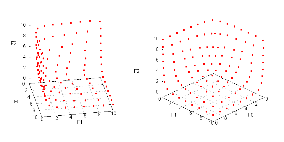
Figure 7. Pareto front for problem (18) consisting of 120 points obtained with 6,264 function evaluations.

We computed evenness values, as well as state the number of function evaluations required per Pareto point, and compare them to reported values from the literature in table 1.

Table 1. Problem (18) Results, A comparison of solution quality (evenness [E]) and computational effort (function evaluations per point [FE/Point]) for problem (18). Reference values for WS, NBIm, and NCm algorithms were obtained from [13]. It is not clear whether the number of function evaluations reported includes those induced by finite difference schemes, or if analytical derivatives were used in the scalar minimizations. Our results were obtained with a first-order finite difference implementation.

Method	E	FE/Point
WS	4.331	120.2
NBIm	0.2958	34.3
NCm	0.2958	34.4
Our new algorithm (15)	0.01930	52.2

5.7. Problem 2

The other problem is an extension of (18) to four objectives.

(19) $$\min\limits_{\textbf{x}}f_{i}(\textbf{x}) = x_{i}\mbox{ for }i=1,2,3,4$$

subject to

$$-x_{1}+x_{2}^{-1}+x_{3}^{-1}+x_{4}^{-1}\leq 0$$

$$x_{1}^{-1}-x_{2}+x_{3}^{-1}+x_{4}^{-1}\leq 0$$

$$x_{1}^{-1}+x_{2}^{-1}-x_{3}+x_{4}^{-1}\leq 0$$

$$x_{1}^{-1}+x_{2}^{-1}+x_{3}^{-1}-x_{4}\leq 0$$

$$0.2\leq x_{i}\leq 10$$

Likewise, with a simplicial CHIM 220-point ansatz, we obtained a smooth, connected Pareto front (figure 8) using two iterations of our algorithm.

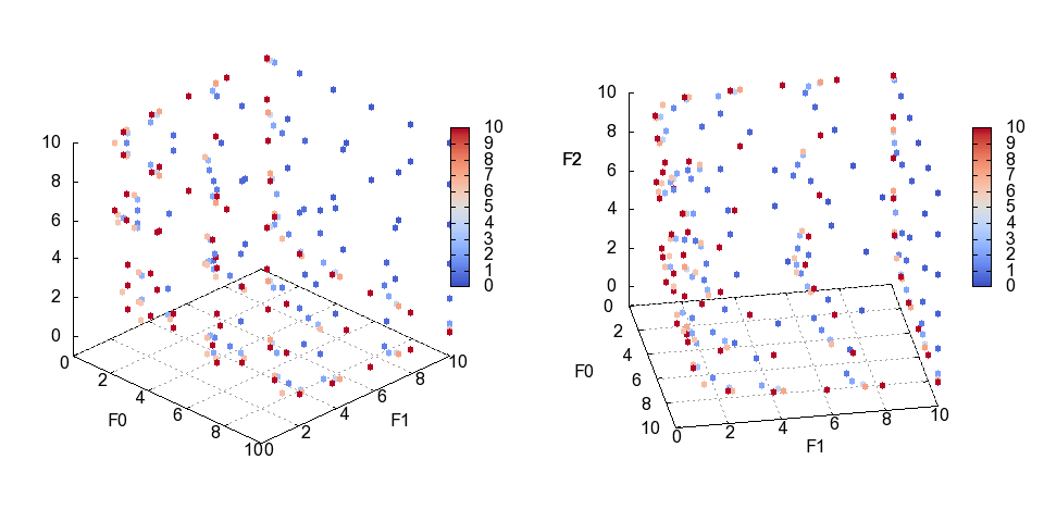
Figure 8. Pareto front for problem (19) consisting of 220 points obtained with 10,670 function evaluations. The value of the fourth objective for each point is shown using the red-blue color-map.

As before, we computed evenness values, and tracked the number of function evaluations required per Pareto point. Table 2 compares the results to reported values from the literature.

Table 2. Problem (19) Results A comparison of solution quality (evenness [E]) and computational effort (function evaluations per point [FE/Point]) for problem (19). Reference values for WS, NBIm, and NCm algorithms were obtained from [13].

, Method E FE/Point WS 4.836 231.9 NBIm 0.3262 49.3 NCm 0.3072 55.3 Our new algorithm (15) 0.02091 48.5

5.8. Problem 3

On the other hand, the EA community tends to focus on different kinds of problems. EAs, being driven by random generation and recombination of solutions, are typically useful in situations where derivative information is unavailable or unhelpful. As a result, test problem suites intended for EAs employ highly non-convex, rapidly oscillating, and extremely discontinuous objectives that are often inappropriate for constraint-based methods, like the one presented here. Therefore, we limit our discussion to a representative example as the primary motivation is to demonstrate the precise equispacing of produced solutions and economy of function evaluations.

(21) $$x\min\limits_{\textbf{x}} f_{i}(\textbf{x})\mbox{ for }i=1,2,3$$

subject to

$$f_{1}(\textbf{x}) = (1+g(x))\cos(x_{1}\pi/2)\cos(x_{2}\pi/2)$$

$$f_{2}(\textbf{x}) = (1+g(x))\cos(x_{1}\pi/2)\sin(x_{2}\pi/2)$$

$$f_{3}(\textbf{x}) = (1+g(x))\sin(x_{1}\pi/2)$$

$$g(\textbf{x}) = \sum_{i=2}^{d}(x_{i}-0.5)^{2}\mbox{ with }0\leq x_{i}\leq 1\mbox{ for }i=1,2$$

We selected a workable problem, defined in (21), from a standard EA test suite [3] and compare the performance to some other heuristics noted in the literature.

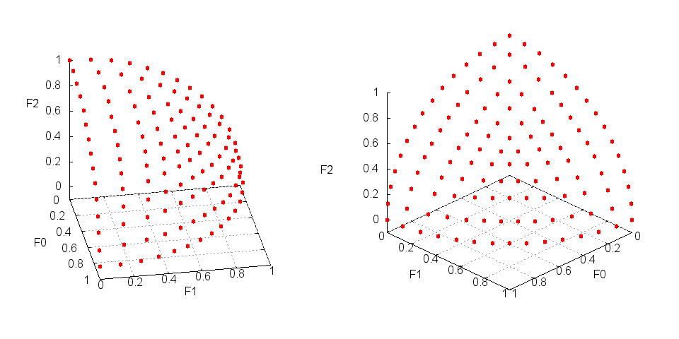
Figure 9. Pareto front for problem (21) consisting of 120 points obtained with 15,765 function evaluations. The finite differences scheme coupled with the fact that the problem has 10 independent variables gives rise to the very high number of function evaluations required. For examples of typical fronts generated by NSGA-II and SPEA2, see [3].

The resulting Pareto front, as seen if figure 9, is computed using significantly fewer function evalutations, obtains a much better hypervolume than any of the algorithms compared in either [15] or [10], and displays more regular sampling than [3].

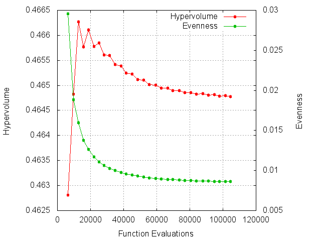
Figure 10. Solution quality metrics for Pareto front for problem (21). Both the solution hypervolume and evenness improve asymptotically as the number of function evaluations increase. In this example, one iteration of algorithm 15 corresponds to about 3,000 function evaluations. The front hypervolume is computed with respect to the origin.

In figure 10, we demonstrate the asymptotic improvement in both hypervolume (computed with respect to the origin) and evenness. This implies that, for certain simple front topologies, algorithm 15 can be terminated after only a few iterations. Moreover, figure 10 shows that further iterations of the algorithm tend to improve the spacing of points more than the obtained hypervolume. This is a result of directly running a set of scalar optimizations (allowing samples to converge to the true optimal front more quickly) rather than ranking and recombining randomly generated solutions.

6. Conclusions

Here, an new algorithm (15) for multi-objective optimization that produces uniformly sampled Pareto fronts by construction is presented. While the algorithm is general, it is most suitable for application to simulation-based engineering optimization problems where economy of function evaluations and smoothness of result are critical. The algorithm discussed achieves an order of magnitude improvement over other geometrically motivated methods, like Normal Boundary Intersection and Normal Constraint, with respect to solution evenness for similar computational expense. This benefit of the proposed method remains, and even improves, after scaling the number of dimensions (and therefore the difficulty of the problem). Furthermore, the resulting uniformity of solutions extends even to more difficult problems, such as those appearing in common EA test cases.

While the resulting discrete representation of the Pareto front, and computational expense of achieving it, are both improved, an other important aspect of the proposed method is its amenability to parallelization. We will report on the parallel aspects together with real world problems [6] in a forthcoming paper.

References

- [1] Das and Dennis. Normal-boundary intersection: A new method for generating the Pareto surface in nonlinear multicriteria optimization problems. SIAM Journal on Optimization, 8(3):631–657, 1998.
- [2] Deb and Pratap. A fast and elitist multiobjective genetic algorithm: NSGA-II. IEEE Transactions on Evolutionary Computation, 6(2):182–197, 2002.
- [3] Deb, Thiele, Laumanns, and Zitzler. Scalable test problems for evolutionary multiobjective optimization. Springer, 2005.
- [4] Deb, Zope, and Jain. Distributed computing of Pareto-optimal solutions using multi-objective evolutionary algorithms. Proceedings of the Second International Conference on Evolutionary Multi-Criterion Optimization, 2003.
- [5] Durillo, Nebro, Luna, and Alba. A study of master-slave approaches to parallelize NSGA-II. 2008 IEEE International Symposium on Parallel and Distributed Processing, pages 1–8, April 2008.
- [6] Ineichen, Adelmann, Kolano, Bekas, Curioni, and Arbenz. A Parallel General Purpose Multi-Objective Optimization Framework, with Application to Beam Dynamics. arXiv:1302.2889 [physics.acc-ph], 2013.
- [7] Ishibuchi, Tsukamoto, Hitotsuyanagi, and Nojima. Effectiveness of scalability improvement attempts on the performance of NSGA-II for many-objective problems. Proceedings of the 10th annual conference on Genetic and evolutionary computation - GECCO ’08, page 649, 2008.
- [8] Jensen. Reducing the Run-Time Complexity of Multiobjective EAs: The NSGA-II and Other Algorithms. IEEE Transactions on Evolutionary Computation, 7(5):503–515, October 2003.
- [9] Leyffer. A Complementarity Constraint Formulation of Convex Multiobjective Optimization Problems. INFORMS Journal on Computing, 21(2):257–267, September 2008.
- [10] Li, Kwong, Cao, Li, Zheng, and Shen. Achieving balance between proximity and diversity in multi-objective evolutionary algorithm. Information Sciences, 182(1):220–242, January 2012.
- [11] Marler and Arora. Survey of multi-objective optimization methods for engineering. Structural and Multidisciplinary Optimization, 26(6):369–395, April 2004.
- [12] Messac and Mattson. Normal constraint method with guarantee of even representation of complete Pareto frontier. AIAA journal, 42(10):2101–2111, 2004.
- [13] Motta, Afonso, and Lyra. A modified NBI and NC method for the solution of N-multiobjective optimization problems. Structural and Multidisciplinary Optimization, 46(2):239–259, January 2012.
- [14] Mueller-Gritschneder. A successive approach to compute the bounded Pareto front of practical multiobjective optimization problems. SIAM Journal on Optimization, 20(2):915–934, 2009.
- [15] Nebro, Durillo, and Coello. A study of convergence speed in multi-objective metaheuristics. Proceedings of the 10th international conference on Parallel Problem Solving, 2008.
- [16] Nebro, Durillo, Luna, Dorronsoro, and Alba. MOCell: A cellular genetic algorithm for multiobjective optimization. International Journal of Intelligent Systems, 24(7):726–746, July 2009.
- [17] Pereyra. Fast computation of equispaced Pareto manifolds and Pareto fronts for multiobjective optimization problems. Mathematics and Computers in Simulation, 79(6):1935–1947, February 2009.
- [18] Pereyra, Saunders, and Castillo. Equispaced Pareto front construction for constrained bi-objective optimization. Mathematical and Computer Modelling, pages 1–10, 2011.
- [19] While, Bradstreet, and Barone. A fast way of calculating exact hypervolumes. IEEE Transactions on Evolutionary Computation, 16(1):86– 95, 2012.
- [20] Zitzler and Thiele. Multiobjective evolutionary algorithms: a comparative case study and the strength Pareto approach. IEEE Transactions on Evolutionary Computation, 3(4):257–271, 1999.