The shrinking figure eight and other solitons for the curve diffusion flow

Abstract.

In this article we investigate the dynamics of special solutions to the surface diffusion flow of idealised ribbons. This equation reduces to studying the curve diffusion flow for the profile curve of the ribbon. We provide: (1) a complete classification of stationary solutions; (2) qualitative results on shrinkers, translators, and rotators; and (3) an explicit parametrisation of a shrinking figure eight curve.

1. Introduction

The curve diffusion flow is a particular evolution law governing the changing shape of a curve in time. It is the one-intrinsic-dimension analogue of the surface diffusion flow for evolving surfaces. These flows are gradient flows of a certain energy functional in a certain function space, but not the more common $L^{2}$-gradient flow such as the curve shortening flow (corresponding to decreasing the length functional for a curve), the mean curvature flow (decreasing the area functional for a surface), or the Willmore flow (decreasing the elastic energy for a curve or the Willmore energy for a surface).

Surface diffusion flow was first described by W. W. Mullins in 1956 as a model for the development of grooving at grain boundaries of heated crystal structures [Mullins]. The flow is also related to the Cahn-Hilliard equation, which describes phase separation and coarsening in the quenching process of binary alloys [CENC]. For further analysis and historical remarks on the surface diffusion flow and its constrained variations we refer the interested reader to [MWW, W1, W2].

The surface diffusion flow is a fourth-order nonlinear parabolic system of equations that, at each time $t$, moves points $p$ on the solution surface $f$ perpendicularly to the surface with speed $(\Delta H)(p)$. Here $\Delta$ is the Laplace-Beltrami operator and $H$ is the mean curvature, which is given by $H=\left\langle\Delta f,\nu\right\rangle$. The inner product $\left\langle\cdot,\cdot\right\rangle$ is the standard dot product in $\mathbb{R}^{3}$.

Surface diffusion flow is the geometric analogue of the classical parabolic clamped plate equation, which expresses the dynamics of a flat plate realised as the graph of a function over a domain in $\mathbb{R}^{2}$. The curve diffusion flow is similarly the geometric analogue of the classical parabolic Euler-Bernoulli model for a clamped rod, modelled as the graph of a function over an interval in $\mathbb{R}$. When the domain is no longer flat, as is the case for a clamped arc segment of a circle in the plane or cylindrical ring in space, the geometry of the problem must enter into the model [ESK, ES]. The surface or curve diffusion flow can capture the notion of stability for an elastic plate or rod under stress respectively. Indeed, if the flow returns all small perturbations of a given initial configuration to that initial configuration without exception, then this configuration is called stable [N].

If the evolving surfaces are cylindrical, as would be the case for idealised closed ribbons with their width extended to infinity, then this remains so under the flow. In this case the flow equation reduces to a one-dimensional parabolic equation for the profile curve $\gamma$. For the surface diffusion flow, this equation is exactly the curve diffusion flow. This reduction is also performed in [ES].

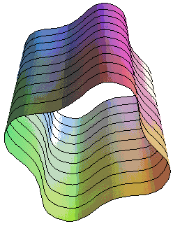
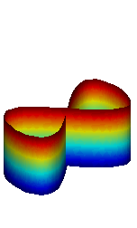
Figure 1. Pieces of two cylindrical ribbons, immersed via $f(u,z)=(x(u),y(u),z)$ where $(u,d)\in\SS\times\mathbb{R}$. The curve $\gamma(u)=(x(u),y(u))$ is called the profile curve. The ribbon on the left is embedded, while the ribbon on the right is immersed. The profile curve of the ribbon on the right is the self-similar figure eight curve we introduce in Section 6.

Let us briefly remark on the above procedure with respect to the particular case of a Möbius band. Extending the width of the Möbius band to infinity must result in self-intersections, and so, the profile curve does not project uniquely to a plane curve in $\mathbb{R}^{2}$. This is an essential characteristic of the Möbius band. One way in which we could overcome this difficulty is instead to immerse the Möbous band in $\mathbb{R}^{4}$, then extend the width to infinity, and project to $\mathbb{R}^{3}$. This would produce a profile curve in $\mathbb{R}^{3}$, the analysis of the dynamics of which are much more complicated than for the planar curve case.

In this paper we concentrate on the dynamics of solutions to the curve diffusion flow which evolve either by scaling, translation or rotation only. These solutions are known as solitons. Solitons are of interest both from a theoretical and practical viewpoint due to their relationship with singularities: given a family of evolving curves, if the family exists for at most a finite amount of time, then it must develop a singularity at the final time. Upon rescaling the flow, effectively ‘zooming in on the singularity’, we expect to construct a family of curves which approximate one of the solitons for the flow.

The existence of finite-time singularities is typically a difficult question, especially in the case of fourth and higher-order curvature flows. For the curve diffusion flow, this was settled in Polden [Polden96]. The analysis there was later extended by Escher and Ito [EI] to more complex initial configurations. In particular, they prove the following theorem.

Theorem 1 (Escher-Ito-Polden).

Let $\gamma_{0}$ be a plane curve with winding number zero. Let $T$ denote the maximal time of existence for the curve diffusion flow $\gamma_{t}:=\gamma(\cdot,t)$ with initial data $\gamma_{0}=\gamma(\cdot,0)$. Then

1. The estimate $T^{*}(\gamma_{0}):=\frac{L^{4}(\gamma_{0})}{64\pi^{4}}\geq T$ holds, where $L(\gamma_{0})$ denotes the length of $\gamma_{0}$; and

2. If $T=T^{*}(\gamma_{0})$ then the solution shrinks to a point as $t$ approaches $T$.

This theorem raises two interesting questions:

1. Is there a solution with winding number zero whose maximal existence time satisfies $T=T^{*}(\gamma)$?

2. Is there a solution with winding number zero that shrinks to a point? (That is, no other kind of singularity occurs.)

The first question investigates the sharpness of the theorem. Its answer is no, since in the proof of Theorem 1, Fenchel’s inequality is used, and for plane curves with winding number zero, it is strict. Furthermore, the upper bound from Theorem 1 may be improved by a factor of $\frac{\pi^{2}}{12}$ by using the following argument.

Let $\gamma_{t}$ be a family of curves evolving by curve diffusion flow. Differentiating the length yields

(1) $$L^{\prime}(\gamma_{t})=-\int_{\gamma}|\partial_{s}\kappa|^{2}d\ell\,,$$

where $\kappa(s)$ is the curvature of $\gamma_{t}$ and $\gamma(t)$ is parametrised by arc length. We use $\partial_{s}$ and $d\ell$ to denote the arc length derivative and element respectively. (We refer the reader to Section 2 for more detail on the notation.) For curves with winding number zero, the curvature $\kappa$ has zero average, and furthermore $\Big{(}\int_{\gamma}|\kappa|\,d\ell\Big{)}^{2}\leq\frac{\pi^{2}}{12}L(\gamma_{t})\int_{\gamma}|\kappa|^{2}d\ell$ (this holds for any function with zero average), so, using the standard sharp Poincaré inequality we compute

$$\bigg{(}\int_{\gamma}|\kappa|\,d\ell\bigg{)}^{2}\leq\frac{\pi^{2}}{12}L\int_{\gamma}|\kappa|^{2}d\ell\leq\frac{\pi^{2}}{12}L\cdot\frac{L^{2}}{4\pi^{2}}\int_{\gamma}|\partial_{s}\kappa|^{2}d\ell=\frac{L^{3}}{48}\int_{\gamma}|\partial_{s}\kappa|^{2}d\ell\,.$$

In the above we have omitted the argument $\gamma_{t}$ from $L$. Since $\lVert\kappa\rVert_{1}:=\int_{\gamma}|\kappa|\,d\ell\geq 2\pi$ (by a simple variant of Fenchel’s theorem), we combine this with (1) above to conclude

$$(L^{4})^{\prime} =4L^{3}L^{\prime}=-4\lVert\partial_{s}\kappa\rVert_{2}^{2}L^{3}\leq-4(48\lVert\kappa\rVert_{1}^{2})\leq-3\cdot 4^{4}\pi^{2}$$

$$\Longrightarrow L^{4}(\gamma_{t}) \leq-3\cdot 4^{4}\pi^{2}t+L^{4}(\gamma_{0})\,,$$

and consequently we obtain the estimate $T\leq\tilde{T}(\gamma_{0}):=L^{4}(\gamma_{0})/768\pi^{2}$, which is better than the estimate given by Theorem 1.

In the above proof, there are three key estimates used: Fenchel’s inequality, the Poincaré inequality, and a sharp Hölder-type inequality for functions with zero average. It is not the case that the same curve satisfies equality for all three of these and therefore it appears clear that the improved bound $T\leq\tilde{T}(\gamma_{0})$ is again not optimal. The broader question therefore on characterising the optimal upper bound on the maximal time of existence in terms of initial length for curves with winding number zero remains open:

1. Is there a $\hat{T}$ depending only on initial length $L(\gamma_{0})$ such that:

   1. All curve diffusion flows with winding number zero have maximal time bounded by $\hat{T}$; and

   2. Does there exist at least one curve diffusion flow with maximal time equal to $\hat{T}$, or, does there exist a sequence of solutions $\gamma_{i}$ with initial data $\gamma_{i}^{(0)}$ and winding number zero whose maximal existence time $T_{i}$ satisfies $|\hat{T}(\gamma_{i}^{(0)})-T_{i}|\rightarrow 0$?

In this paper we shall not answer this question. We do however provide an answer to the second question (2) above. The second question is interesting from a classification of finite-time singularities perspective. The key issue there is to demonstrate that solutions may become singular by simply becoming small – a rescaling of such solutions will exist for all time and be asymptotic to a smooth model curve. A finite-time singularitiy of this type is said to be of Type I, in analogy with existing work on the mean curvature flow [Hu]. Other singularities are called Type II. Type I singularities are expected to be simpler in structure and satisfy natural stability criteria when compared with Type II singularities.

We answer the second question in the affirmative by way of an explicit example: a self-similarly shrinking immersed figure eight. This figure eight is in fact the lemniscate of Bernoulli. Since one requires zero area to have the possibility that the solution shrinks to a point (see Lemma 5), and the maximal existence time is finite (see Theorem 1), a figure eight with one leaf smaller than the other will certainly become singular with non-zero area, ruling out the possibility that it is asymptotic to a point.

Let $\gamma$ be the shrinking figure eight described in Section 6. Upon scaling $\gamma$ to satisfy $L(\gamma)=1$, we compute the extinction time of the flow to be

$$T=\frac{1}{3\cdot 2^{11}\cdot\mathcal{K}(-1)^{4}}\,,$$

where $\mathcal{K}(m)$ is the complete elliptic integral of the first kind with parameter $m=k^{2}$. In this particular case the maximal time estimate $T^{*}$ overshoots $T$ by a factor of roughly 2.9, and $\tilde{T}$ overshoots $T$ by a factor of roughly 2.4:

$$\frac{T^{*}}{T}=2.9115257845\ldots\,,\qquad\frac{\tilde{T}}{T}=2.3946339747\ldots\,.$$

In a sense, the self-similar figure eight represents a “best-case” scenario. The generic case is that an arbitrary smooth curve with winding number zero will be driven to a curvature singularity and not shrink to a point. Furthermore, such a singularity involves blowup of the curvature and its derivatives, so in particular the speed of the flow is greater in this circumstance. These heuristics lead us to make the following conjecture.

Conjecture.

The maximal existence time of a curve diffusion flow emanating from a curve with winding number zero is bounded by the existence time of a self-similar figure eight with the same initial length.

Of course, verifying the conjecture has uniqueness of the self-similar figure eight as a corollary.

Another popular fourth-order surface evolution equation is the Willmore flow, whose one-dimensional counterpart, the elastic flow, also models cylindrical elastic ribbons. The key difference between the two flows is that the elastic flow minimises the integral of the square of the curvature of the curve, while the curve diffusion flow minimises length, keeps enclosed volume fixed, and keeps the quantity

$$\mathcal{Q}(t)=\int_{0}^{t}\bigg{(}\int_{\gamma}|\partial_{s}\kappa|^{2}\,d\ell\bigg{)}\,dt$$

uniformly bounded, with a bound dependent only on the initial data. A proof of these statements can be found in [Wheeler]. We remark on the similarities and differences between this flow and the curve diffusion flow throughout this article.

The structure and specific contributions of this article are as follows. We begin Section 2 by setting up notation, defining key geometric quantities and giving the fourth-order nonlinear parabolic system of partial differential equations for the curve diffusion flow. We then briefly review relevant previous work and the question of local existence before moving on to a classification of stationary solutions – those that remain constant under the flow. We provide a five-parameter family of parametrisations which completely classifies these solutions. In Section 3 we record some elementary properties of the flow that are relevant to our investigations. In Section 4 we focus on curves that evolve self-similarly, deriving the corresponding fourth-order ordinary differential equation satisfied by such curves. We prove several properties of self-similar solutions. Section 5 is devoted to curves that evolve by translation only. We prove there that the only closed translators are circles, and that the only open translators (open immersions of $\mathbb{R}$) satisfying either of two conditions at infinity are straight lines. In Section 6 we provide an explicit parametrisation of a figure eight immersed curve and verify that this curve does indeed evolve self-similarly under the curve diffusion flow, contracting to a point in finite time. In Section 7 we consider the case of rotating solutions and prove some non-existence results analogous to those for translators in Section 5.

2. The curve diffusion flow equation

We will parametrise closed evolving curves over the unit circle $\mathbb{S}$, and open evolving curves over the real line $\mathbb{R}$. Let $\gamma$ denote the evolving curve, with components

$$\gamma\left(u\right)=\left(x\left(u\right),y\left(u\right)\right)\mbox{.}$$

The tangent direction to the curve is given by

$$\gamma_{u}\left(u\right)=\left(x_{u}\left(u\right),y_{u}\left(u\right)\right)\mbox{,}$$

and therefore a choice of unit normal is

$$\nu\left(u\right)=\frac{1}{\left|\gamma_{u}\left(u\right)\right|}\left(y_{u}\left(u\right),-x_{u}\left(u\right)\right)\mbox{,}$$

where $\left|\cdot\right|$ denotes the length of a vector. We will always assume our curves are smooth and regular, that is, $\left|\gamma_{u}\right|>0$ for all $u$. Recall that, in a general parametrisation, the arc length of a curve $\gamma$, beginning at point $\gamma\left(u_{0}\right)$, is given by

(2) $$s\left(u\right)=\int_{u_{0}}^{u}\left|\gamma_{u}\left(\tilde{u}\right)\right|d\tilde{u}\mbox{.}$$

The arc length induces an arc length element $d\ell=|\gamma_{u}|\,du$. The curvature vector and curvature of a plane curve is given by

$$\vec{\kappa}=\gamma_{ss}\quad\text{and}\quad\kappa=\left\langle\nu,\vec{\kappa}\right\rangle\,,$$

where we use $\left\langle\cdot,\cdot\right\rangle$ to denote the standard inner product between vectors in the plane. For closed embedded curves, we will always choose an inward-pointing unit normal, so that the curvature of a circle is positive. Otherwise, we select either normal – the curve diffusion flow is invariant under changes in orientation.

We say $\gamma_{t}=\gamma(\cdot,t)$ evolves under the curve diffusion flow if it satisfies the system of fourth-order partial differential equations

(3) $$\frac{\partial\gamma}{\partial t}\left(u,t\right)=-\kappa_{ss}\left(u,t\right)\nu\left(u,t\right)\quad\mbox{for}\quad\left(u,t\right)\in\mathbb{S}\times\left(0,T\right)$$

with initial condition

$$\gamma\left(u,0\right)=\gamma_{0}\left(u\right)\mbox{,}$$

for some given initial curve immersion $\gamma$. Note that an immersed curve may have intersections, however, it has a well-defined tangent vector for each $u$. We label the maximal existence time of a solution to (3) as $T$.

We are interested in the shape of the evolving curves, that is, the image $\gamma(\SS,t)$ for closed solutions, or $\gamma(\mathbb{R},t)$ for open solutions, as a set in $\mathbb{R}^{2}$, and not in the orbit of a specific point. There is a degeneracy in the flow equation (3): reparametrisation and tangential movement of points in the direction of $\gamma_{s}$ do not affect the shape of the image $\gamma(\SS,t)$. The degeneracy consists of every diffeomorphism $\varphi:\SS\rightarrow\SS$. This implies that, in terms of the images $\gamma(\SS,t)$, the flow (3) is equivalent to

(4) $$\left\langle\frac{\partial\gamma}{\partial t}\left(u,t\right),\nu(u,t)\right\rangle=-\kappa_{ss}\left(u,t\right)\quad\mbox{for}\quad\left(u,t\right)\in\mathbb{S}\times\left(0,T\right)$$

The impact of this observation on our analysis here is that when considering solutions with a particular form, we must also take into account a possible diffeomorphism $\varphi$ acting on $\SS$. This typically forces us to take normal projections in order to remove the influence of $\varphi$.

Note that

$$\kappa_{ss}=\partial_{s}^{2}\left\langle\gamma_{ss},\nu\right\rangle=\frac{1}{|\gamma_{u}|}\Bigg{(}\frac{1}{|\gamma_{u}|}\bigg{(}\left\langle\frac{1}{|\gamma_{u}|}\Big{(}\frac{\gamma_{u}}{|\gamma_{u}|}\Big{)}_{u},\nu\right\rangle\bigg{)}_{u}\Bigg{)}_{u}$$

so that the leading order term of $-\kappa_{ss}=\left\langle\partial_{t}\gamma,\nu\right\rangle$ is precisely

$$-\frac{1}{|\gamma_{u}|^{4}}\left\langle\gamma_{uuuu},\nu\right\rangle\,.$$

The normal direction is ‘positive’ for the flow (3), and so this shows that (3) is a quasilinear parabolic system.

Current understanding of the curve diffusion flow is quite limited, apart from short time existence. There are several methods for obtaining short time existence of solutions to (3) given suitable initial data; we refer the reader to the discussion of these in [Wheeler] and the references contained therein. Very little else is known about the behaviour of the flow. Giga and Ito [GI1] provided an example of a simple, closed, embedded plane curve that develops a self-intersection in finite time under the flow (3). They also gave an example in [GI2] of a closed, strictly convex plane curve that becomes non-convex in finite time. Elliot and Maier-Paape showed that curves that are initially graphical may evolve under (3) to become non-graphical in finite time [EMP]. On the other hand, the fourth author recently showed [Wheeler] that under the curve diffusion flow, solution curves that are initially close to a circle, in the sense of the normalised integral of the square of the oscillation of curvature, exist for all time and converge exponentially fast to a (possibly different) circle. Further, those admissible curves which are initially embedded remain embedded. A fundamental obstacle in the analysis of such flows and of (3) is that, as a system of higher order partial differential equations, arguments based upon maximum principles are in general not available.

Let us now move on to the classification of stationary curve diffusion flows. We call the family of curves $\gamma(\cdot,t)$ a closed solution if $\gamma$ satisfies (4) and $\gamma(u)=\gamma(u+P)$ for some $P>0$. The smallest such $P$ is the period of $\gamma$.

A solution is called stationary if it does not change in time under (4), that is, if $\kappa_{ss}(u,t)\equiv 0$.

Lemma 2.

Suppose $\gamma:\SS\rightarrow\mathbb{R}^{2}$ is a closed stationary solution to the curve diffusion flow. Then $\gamma$ is a round circle.

Proof: Integrating by parts and using $\kappa_{ss}=0$ we have

$$0=-\int_{\gamma}\kappa\,\kappa_{ss}\,d\ell=\int_{\gamma}\kappa_{s}^{2}\,d\ell$$

and so $\kappa_{s}=0$, that is, $\kappa$ is constant. Therefore $\gamma$ is a smooth closed curve with constant curvature, and by the classification of curves in $\mathbb{R}^{2}$, any curve with constant curvature in the plane is a straight line or round circle. Since $\gamma$ is closed, $\gamma$ can not be a straight line, and so it must be a round circle. $\Box$

The situation is more complicated for open solutions. We define an open curve to be a regular immersion $\gamma:\mathbb{R}\rightarrow\mathbb{R}^{2}$ of $\mathbb{R}$ for which there does not exist a pair of intervals $I$, $J$ such that

(5) $$I\cap J=\emptyset\,,\quad|I|=\infty\,,\quad|J|<\infty\,,\quad\text{and}\quad\gamma(I)=\gamma(J)\,.$$

This last condition captures the notion of not allowing $\gamma$ to ‘close’ while still allowing infinitely many self-intersections, including possibly intersecting on an arbitrarily large open set.

Open curves may concentrate around a particular point, such as a logarithmic spiral. This concentration behaviour is encapsulated by the notion of properness of the curve $\gamma:\mathbb{R}\rightarrow\mathbb{R}^{2}$. The curve $\gamma$ is proper if for any compact set $C\subset\mathbb{R}^{2}$ the inverse image

$$\gamma^{-1}(C):=\{u\in\mathbb{R}:\gamma(u)\in C\}$$

is a compact set.

Lemma 3.

Suppose $\gamma:\mathbb{R}\rightarrow\mathbb{R}^{2}$ is an open stationary solution to the curve diffusion flow. Then $\gamma$ is either a straight line, or a similarity transformation of the standard Cornu spiral. Up to translation and rotation such curves satisfy

$$\kappa(s)=k_{2}s+k_{1}$$

for a pair $(k_{1},k_{2})\in\mathbb{R}^{2}$.

Proof: If $\kappa_{ss}=0$, then there is a $k_{2}\in\mathbb{R}$ such that

$$\kappa_{s}(s)=k_{2}\,.$$

The curvature $\kappa$ is therefore linear in $s$; that is, there exists a $k_{1}\in\mathbb{R}$ such that

$$\kappa(s)=k_{2}s+k_{1}\,.$$

If $k_{2}\neq 0$, then after reparametrising by $t=s+\frac{k_{1}}{k_{2}}$ we have

$$\kappa(t)=k_{2}t\,.$$

Furthermore, by scaling the curve $\gamma$ by a factor of $\sqrt{k_{2}}/\sqrt{\pi}$ we have

$$\hat{\kappa}(t)=\frac{\sqrt{\pi}}{\sqrt{k_{2}}}\kappa(t)=\sqrt{k_{2}\pi}t=\pi\hat{t}\,.$$

Therefore either $k_{2}=0$, in which case we have a straight line, or $k_{2}\neq 0$ and we have a similarity transformation of the standard Cornu spiral. $\Box$

Remark: Combining the above two lemmata, we see that up to similarity transformations the only three stationary solutions are the circle, straight line, and Cornu spiral.

Corollary 4.

Suppose $\gamma:\mathbb{R}\rightarrow\mathbb{R}^{2}$ is an open, stationary, properly immersed solution to the curve diffusion flow. Then $\gamma$ is a straight line.

Proof: We apply Lemma 3 above to obtain that $\gamma$ has curvature satisfying

$$\kappa(s)=k_{2}s+k_{1}\,.$$

If $k_{2}=0$ then $\kappa$ is a constant and so $\gamma$ is a straight line, as required.

Suppose on the contrary that $k_{2}\neq 0$. We will show that this leads to a contradiction to the properness assumption. Consider the restriction $\hat{\gamma}$ of $\gamma$ to the interval $(0,\infty)$ if $k_{2}>0$ or to the interval $(-\infty,0)$ if $k_{2}<0$. The curve $\hat{\gamma}$ has strictly monotone positive curvature. We may therefore apply the classical Tait-Kneser theorem to obtain that the osculating circles of $\hat{\gamma}$ are pairwise disjoint and nested (see [GTT] and the references therein for a discussion of Tait’s original paper and some interesting extensions). Recall that the osculating circle at $\gamma(s_{0})$ is the best approximating circle to $\gamma(s_{0})$. It is a standard round circle with radius $1/\kappa(s_{0})$ and centre $(\gamma(s_{0})+\nu(s_{0})/\kappa(s_{0}))$.

Let $\mathcal{C}(s_{0})$ denote the osculating circle at $\hat{\gamma}(s_{0})$ and $\mathcal{D}(s_{0})$ denote the disk with boundary $\mathcal{C}(s_{0})$. The theorem implies that

$$\mathcal{D}(s_{0})\supset\bigcup_{s\in[s_{0},\infty)}\mathcal{C}(s)\supset\bigcup_{s\in[s_{0},\infty)}\gamma(s)\,.$$

Clearly $\mathcal{D}(s_{0})$ is compact. The above computation shows that

$$\gamma^{-1}(\mathcal{D}(s_{0}))=[s_{0},\infty)\,,$$

which is not compact, and so $\gamma$ is not proper. This is contrary to the hypotheses of this Corollary, and so $k_{2}=0$, as required. $\Box$

The two-parameter family of open curves given by Lemma 3 therefore consists of a particular family of improperly immersed curves and straight lines. The improperly immersed curves are Eulerian spirals, with the clothoid or Cornu spiral ($k_{2}=\pi$ and $k_{1}=0$) a standard example. The arc length parametrisation of the clothoid is given in terms of the Fresnel $C$ and $S$ integrals:

$$\gamma(s)=(\,C(s),S(s)\,)\,,\quad\text{where}\quad C(s)=\int_{0}^{s}\cos\Big{(}\frac{\pi t^{2}}{2}\Big{)}\,dt\quad\text{and}\quad S(s)=\int_{0}^{s}\sin\Big{(}\frac{\pi t^{2}}{2}\Big{)}\,dt\,.$$

The curvature of the clothoid is $\kappa(s)=s\pi$. In order to produce the whole two-parameter family, let us define the modified Fresnel integrals $C(s,c_{1},c_{2})$ and $S(s,c_{1},c_{2})$ by

$$C(s,c_{1},c_{2})=\int_{0}^{s}\cos\big{(}c_{1}t+c_{2}t^{2}\big{)}\,dt\quad\text{and}\quad S(s,c_{1},c_{2})=\int_{0}^{s}\sin\big{(}c_{1}t+c_{2}t^{2}\big{)}\,dt\,.$$

The curve $\gamma:\mathbb{R}\rightarrow\mathbb{R}^{2}$ with arc length parametrisation

$$\gamma(s)=(\,C(s,c_{1},c_{2}),S(s,c_{1},c_{2})\,)$$

then has curvature $\kappa(s)=2sc_{2}+c_{1}$.

Note that this includes the case of circles ($c_{2}=0$) and straight lines ($c_{1}=c_{2}=0$). The curvature $\kappa$ is invariant under rigid motions (rotations and translations), and therefore in order to account for the entire family of stationary solutions we must include all possible rotations and translations of the model members $\gamma(s)=(\,C(s,c_{1},c_{2}),S(s,c_{1},c_{2})\,)$. Therefore the family $\mathcal{F}$ of immersed open or closed stationary solutions to the curve diffusion flow consists precisely of the five parameter family

$$\mathcal{F}=\Bigg{\{}\gamma(s)=\bigg{[}\bigg{(}\begin{matrix}\cos\theta&-\sin\theta\\ \sin\theta&\cos\theta\end{matrix}\bigg{)}\bigg{(}\begin{matrix}C(s,c_{1},c_{2})\\ S(s,c_{1},c_{2})\end{matrix}\bigg{)}\bigg{]}^{T}+(V_{1},V_{2})\text{ for some }(c_{1},c_{2},V_{1},V_{2},\theta)\in\mathbb{R}^{4}\times\SS\Bigg{\}}\,,$$

up to reparametrisation. Some members of $\mathcal{F}$ are depicted in Figure 2.

Remark (Elastic flow): We say $\gamma_{t}$ evolves under the elastic flow if $\gamma(\cdot,t)=\gamma_{t}$ satisfies

$$\frac{\partial\gamma}{\partial t}(u,t)=\Big{(}-\kappa_{ss}(u,t)-\frac{1}{2}\kappa^{3}(u,t)\Big{)}\nu(u,t)\,.$$

The elastic flow is the steepest descent $L^{2}$-gradient flow of $\int_{\gamma}\kappa^{2}\,d\ell$. For global regularity results and further historical references we refer to [DKS]. Stationary solutions are termed elasticae and satisfy

$$\kappa_{ss}(u,t)=-\frac{1}{2}\kappa^{3}(u,t)\,.$$

A classification of solutions to this equation is not yet known in the sense discussed here, that is, in terms of explicit parametrisations. Indeed, there are no known closed solutions to this equation. Open solutions are yet to be classified. We conjecture that there are no open properly immersed solutions apart from the straight line.

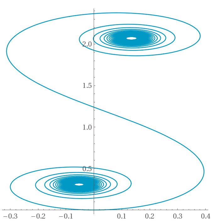
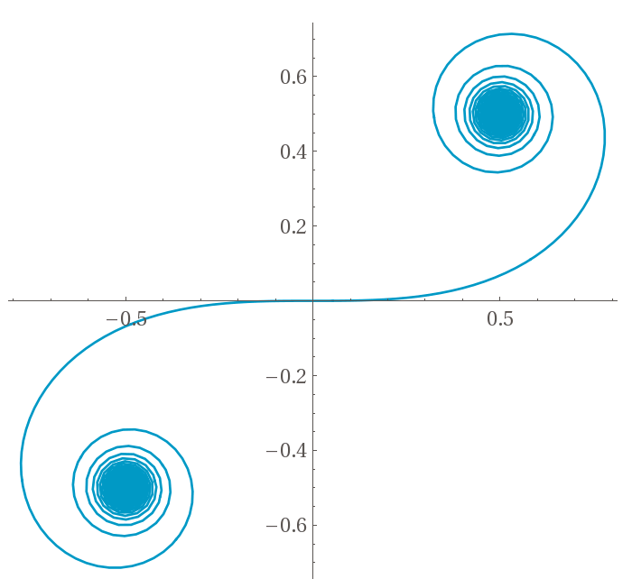
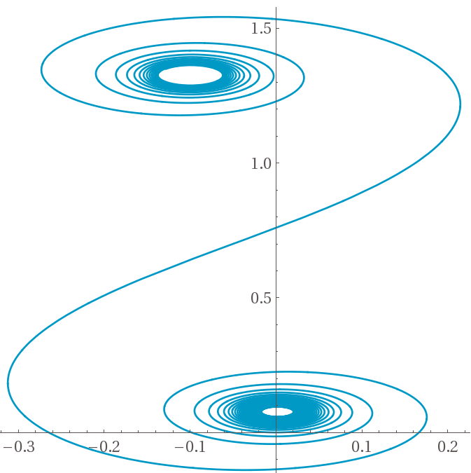
Figure 2. Three members of $\mathcal{F}$: the left with $\kappa(s)=-2s+3$, the middle with $\kappa(s)=s$, and the right with $\kappa(s)=4s+13$. We choose $(\theta,V_{1},V_{2})=(0,0,0)$ for each.

3. Elementary properties of the curve diffusion flow

In this section we examine the behaviour of the arc length of $\gamma_{t}$, and the area enclosed within $\gamma_{t}$, under the flow (3). Because $\gamma_{t}$ may be an immersed curve, care is required in defining the enclosed area, or simply the change in enclosed area; we refer the reader to the discussion in [MW] for details (that article concerns evolving immersed surfaces and discusses the definition of the signed enclosed volume, but the issues are analogous). When the curve $\gamma_{t}$ is an embedded curve, the calculations below are the one intrinsic dimension analogues of those in [M1], for example. The full details for the specific case of the curve diffusion flow of immersed curves are given in [Wheeler].

Lemma 5.

Under the flow (3), the area enclosed by the curve $\gamma_{t}$ remains constant. In particular, if the family of curves $\gamma_{t}$ contract to a point, then the initial data $\gamma_{0}$ must have zero signed area.

Proof: The signed area $A\left(\gamma_{t}\right)$ enclosed by $\gamma_{t}$ evolves under (3) according to

$$\frac{d}{dt}A\left(\gamma_{t}\right)=-\int_{\gamma}\kappa_{ss}\,d\ell=0\mbox{.}$$

That is, $A\left(t\right)$ is constant under the flow.

Since the area of a point is zero, and the enclosed area is constant under the flow, the area at any time along a family of curves that contract to a point is zero. In particular, the area of the initial data $\gamma_{0}$ must be zero. $\Box$

Lemma 6.

Under the flow (3), the length of the evolving curve $\gamma_{t}$ is monotone nonincreasing.

Proof: Under the flow (3), the length of the evolving curve $\gamma$ evolves according to

$$\frac{d}{dt}L\left(t\right)=\int_{\gamma}\kappa_{ss}\kappa\,d\ell=-\int_{\gamma}\kappa_{s}^{2}\,d\ell\leq 0\mbox{,}$$

that is, the length is nonincreasing. $\Box$

The above lemmata make the curve diffusion flow interesting from an isoperimetric point of view. In particular, the isoperimetric ratio is monotonically decreasing:

Corollary 7.

The signed isoperimetric ratio

$$I(\gamma_{t})=\frac{L^{2}(\gamma_{t})}{4\pi A(\gamma_{t})}$$

is decreasing in absolute value with value given by

$$I(\gamma_{t})=I(\gamma_{0})e^{-\int_{0}^{t}\frac{2}{L(\gamma_{t})}\int_{\gamma}\kappa_{s}^{2}\,d\ell\,d\tau}\,.$$

Proof: Differentiate $I$ and apply Lemmata 5 and 6 to obtain

$$\frac{d}{dt}I(\gamma_{t})=-\frac{2I(\gamma_{t})}{L(\gamma_{t})}\int_{\gamma}\kappa_{s}^{2}\,d\ell\,.$$

Integrating yields the result. $\Box$

Remark (Elastic flow): Although the elastic flow reduces $\int_{\gamma}\kappa^{2}\,d\ell$ with velocity

$$\frac{d}{dt}\int_{\gamma}\kappa^{2}\,d\ell=-2\int_{\gamma}\Big{|}\kappa_{ss}+\frac{1}{2}\kappa^{3}\Big{|}^{2}\,d\ell\,,$$

the behaviour of the length, area, and isoperimetric ratio, are for generic initial data unknown.

4. Curves evolving homothetically

A self-similar solution to a curvature flow equation is a solution whose image maintains the same shape as it evolves, that is, it changes in time only by scaling, translation and/or rotation. In this section we focus on the case where $\gamma$ evolves by scaling, and in the next section we study solutions which evolve by translation. Section 7 studies curves evolving by rotation.

Closed, self-similar solution hypersurfaces of positive mean curvature for the mean curvature flow are known to be spheres [Hu]; the third author generalised this result for a class of fully nonlinear curvature flows in [M4]. In the corresponding case of the curve shortening flow, self-similar curves were classified in [AL].

Definition.

We say $\gamma_{t}$ is a solution of (3) (or equivalently (4)) evolving homothetically if and only if there is a differentiable function of time $f$ and an initial curve $\gamma_{0}$ such that

$$\gamma\left(u,t\right)=f\left(t\right)\gamma_{0}\left(u\right)\,.$$

This is equivalent to

$$\left\langle\partial_{t}\gamma,\nu\right\rangle=f^{\prime}\left\langle\gamma_{0},\nu\right\rangle\,.$$

In general, homothetic solutions may be expanding, shrinking, stationary, or exhibit more complex breathing behaviour. For the case of curve diffusion flow, Lemmata 5 and 6 show that any solution must decrease its length monotonically (and be asymptotic to a curve with constant curvature unless it exists only for a finite amount of time). We therefore term a homothetic solution $\gamma$ a shrinker or shrinking solution. We take $f\left(0\right)=\rho$ where $\rho\in\mathbb{R}$ as initial condition. This freedom will be useful when we estimate the maximal existence time of the shrinking figure eight in Section 6.

The simplest example of a closed shrinking curve which is a solution to (3) is the circle.

Lemma 8.

Let $\gamma$ be defined by $\gamma\left(u,t\right)=R\left(\cos u,\sin u\right)$ for some constant $R>0$. Then $\gamma$ is a solution to (3).

Proof: We simply observe

$$\frac{\partial\gamma}{\partial t}\left(u,t\right)=\frac{\partial}{\partial t}R\left(\cos u,\sin u\right)=0$$

and since the curvature $\kappa$ of $\gamma$ is identically equal to $\frac{1}{R}$,

$$\kappa_{ss}\left(u,t\right)\equiv 0\mbox{.}$$

Hence (3) is trivially satisfied. $\Box$

If a curve is evolving homothetically under (3), we may write down a corresponding ODE by ‘separation of variables’ that it must satisfy.

Lemma 9.

Let $\gamma:\mathbb{S}\rightarrow\mathbb{R}^{2}$ be a curve. Then $\gamma$ is a self-similar solution to (3) iff there is a constant $K$ such that

(6) $$\kappa_{ss}\left(u\right)=K\left<\gamma\left(u\right),\nu\left(u\right)\right>$$

for all $u\in\mathbb{S}$.

Proof: Suppose the curve $\gamma$ is such that $\gamma\left(u,t\right)=f\left(t\right)\gamma_{0}\left(u,t\right)$ for some positive differentiable function $f\left(t\right)$ with $f\left(0\right)=\rho$, that is, at the initial time $t=0$, $\gamma\left(u,0\right)=\rho\,\gamma_{0}\left(u\right)$. Geometric quantities associated to $\gamma$ are related to those of $\gamma_{0}$ as follows. In the calculations here we often omit the arguments of $\gamma$, $\gamma_{0}$ and $f$. The tangent direction is

$$\gamma_{u}=f\,\partial_{u}\gamma_{0}$$

and the unit normal is

$$\nu=\nu_{0}\,.$$

Above and in what follows we will include a zero subscript on geometric quantities associated with $\gamma_{0}$. The curvature of $\gamma$ is related to that of $\gamma_{0}$ by

(7) $$\kappa=f^{-1}\kappa_{0}\,.$$

In view of (2), the arc length of the curves $\gamma$ and $\gamma_{0}$ are related via

$$s=fs_{0}$$

and so differentiating (7) twice, we find

$$\kappa_{ss}=f^{-3}\partial^{2}_{s_{0}s_{0}}\kappa_{0}\,.$$

Using the above we find that (3) is satisfied if and only if

$$f^{\prime}\left\langle\gamma_{0},\nu_{0}\right\rangle=-f^{-3}\partial^{2}_{s_{0}s_{0}}\kappa_{0}\left\langle\nu_{0},\nu_{0}\right\rangle\,.$$

Following a standard separation of variables argument (note that any zeros of $\left\langle\gamma_{0},\nu_{0}\right\rangle$ are isolated unless $\gamma$ is a straight line passing through the origin – this case is trivial and can be treated separately), there must be a constant $K$ such that

$$(f^{4})^{\prime}=-4\frac{\partial^{2}_{s_{0}s_{0}}\kappa_{0}}{\left\langle\gamma_{0},\nu_{0}\right\rangle}=4K\,.$$

Simplifying this equation finishes the proof.$\Box$

Remarks:

1. Solving the ordinary differential equation for $f$ in the above proof, we have

   $$f\left(t\right)=\sqrt[4]{\rho^{4}+4\,K\,t}\mbox{.}$$

   Assuming also that (6) is satisfied, we observe that

   • If $K=0$, then $f\left(t\right)\equiv 1$ and the curve $\gamma$ is static under (3), that is, a stationary solution that exists for all time $t$.

   • If $K<0$, then the solution to (3) shrinks self-similarly to a point at time $T=-\frac{\rho^{4}}{4K}$.

   • If $K>0$ then any self-similar solution would have to expand indefinitely. However, for closed curves this is not possible in view of Lemma 6. For open curves this is possible, and there could be open expanding solutions. These could be important models for how the curve diffusion flow smooths out isolated singularities, in the same way that the error function generates a self-similar solution to the heat equation with the Heaviside step function as initial data.

2. Clearly, the shrinker condition (6) is invariant under translation and rotation; that is, applying these operations yields another solution to (6) with the same constant $K$. Under scaling by a factor $\rho$, one again obtains a solution to (6), but with a new constant $\hat{K}=K\rho^{4}$. One may express the ODE (6) in terms of a pair of equations for $(x(u),y(u))$ in the original (non-arclength) parametrisation, and apply a standard Lie symmetry analysis to the system. The result of this analysis is that there are no other possible transformations that one may apply in order to obtain more solutions.
   

Remark (Elastic flow): One naturally expects expanders for the elastic flow, in contrast with the shrinkers of curve diffusion flow. The solution to the elastic flow with initial data equal to a circle expands under the flow for all time, and so the standard round circle is the canonical example of an expander. Indeed, Theorems 3.2 and 3.3 of [DKS] establish global existence and convergence to an elastica under the condition that the length of the evolving curves remain fixed. Without this constraint, it appears impossible to obtain convergence of the flow in any sense, since there is no way to control the length. There are no other known expanders for the elastic flow.

5. Curves evolving by translation

A family of curves $\gamma:\SS\times[0,T)\rightarrow\mathbb{R}^{2}$ evolving purely by translation satisfies

(8) $$\frac{\partial\gamma}{\partial t}\left(u,t\right)=\gamma_{0}\left(u\right)+Vt+\gamma_{s}(u,t)\phi(u,t)$$

for some constant vector $V$ and smooth diffeomorphism $\phi$. In this case

$$\left\langle\frac{\partial\gamma}{\partial t},\nu\right\rangle=\left\langle V,\nu\right\rangle\mbox{,}$$

and if (3) is to hold then $\gamma$ must satisfy

(9) $$-\kappa_{ss}\equiv\left\langle V,\nu\right\rangle\mbox{.}$$

We call the solution $\gamma$ a translator. If $V=0$, then the solution $\gamma$ is stationary, and we call the translator trivial.

It is common that for a given curvature flow there are no closed non-trivial translators. Nevertheless one typically expects open immersed non-trivial translating solutions. A family of open immersed curves $\gamma:\mathbb{R}\times[0,T)\rightarrow\mathbb{R}^{2}$ evolving purely by translation satisfies (8) and (9) as in the closed setting. Such curves usually arise as blowup limits of a Type 2 singularity [GageHamilton]. Singularities of this type have engendered much interest in the literature.

In this section we investigate translators for the curve diffusion flow. We prove by a simple argument that there are no smooth closed non-trivial translators. Our proof implies a stronger statement about open curves, which is sharp, by the earlier example of the clothoid.

Proposition 10.

Let $\gamma:\SS\rightarrow\mathbb{R}^{2}$ be a smooth closed translator. Then $\gamma$ is trivial; that is, $\gamma(\SS)$ is a standard round circle.

Proof: Since $\gamma$ is closed, integration by parts gives

(10) $$-\int_{\gamma}\kappa\kappa_{ss}\,d\ell=\int_{\gamma}\kappa_{s}^{2}d\ell\,.$$

Also, noting that $V$ is a constant vector and that the curvature vector $\vec{\kappa}$ satisfies $\kappa\nu=\vec{\kappa}=\gamma_{ss}$, we have

(11) $$\int_{\gamma}\left\langle V,\vec{\kappa}\right\rangle\,d\ell=\int_{\gamma}\partial_{s}\big{(}\left\langle V,\gamma_{s}\right\rangle\big{)}\,d\ell=0\,.$$

Multiplying (9) by $\kappa$ and integrating gives

$$-\int_{\gamma}\kappa\kappa_{ss}\,d\ell=\int_{\gamma}\left\langle V,\vec{\kappa}\right\rangle\,d\ell\,,$$

which when combined with (10) and (11) above yields

$$\int_{\gamma}\kappa_{s}^{2}d\ell=0\,.$$

Since $\gamma$ is smooth, this implies that $\kappa_{s}\equiv 0$ on $\gamma$, that is, that the curvature is constant. Therefore $\kappa_{ss}=0$, and so $V=0$; that is, the translator is trivial. By Lemma 2, it is a round circle. $\Box$

Now let us investigate open curves.

Proposition 11.

Suppose $\gamma:\mathbb{R}\rightarrow\mathbb{R}^{2}$ is a smooth open translator satisfying

(12) $$\lim_{i\rightarrow\infty}\Big{[}\big{(}\kappa(p_{i})\kappa_{s}(p_{i})+\left\langle V,\gamma_{s}(p_{i})\right\rangle\big{)}-\big{(}\kappa(q_{i})\kappa_{s}(q_{i})+\left\langle V,\gamma_{s}(q_{i})\right\rangle\Big{)}\Big{]}=0$$

for arbitrary sequences $\{p_{i}\}$ and $\{q_{i}\}$ asymptotic to $-\infty$ and $+\infty$ respectively. Then $\gamma(\mathbb{R})$ is a straight line.

Proof: Let us follow the idea of Proposition 10. We integrate (9) against $\kappa$ to find

$$\int_{p_{i}}^{q_{i}}\kappa_{s}^{2}d\ell =-\int_{p_{i}}^{q_{i}}\kappa\kappa_{ss}\,d\ell+\kappa\kappa_{s}\big{|}_{p_{i}}^{q_{i}}$$

$$=\int_{p_{i}}^{q_{i}}\left\langle V,\vec{\kappa}\right\rangle\,d\ell+\kappa\kappa_{s}\big{|}_{p_{i}}^{q_{i}}$$

$$=\int_{p_{i}}^{q_{i}}\partial_{s}\big{(}\left\langle V,\gamma_{s}\right\rangle\big{)}\,d\ell+\kappa\kappa_{s}\big{|}_{p_{i}}^{q_{i}}$$

$$=\Big{[}\left\langle V,\gamma_{s}\right\rangle+\kappa\kappa_{s}\Big{]}_{p_{i}}^{q_{i}}\,.$$

Taking $i\rightarrow\infty$ yields the result. Note that circles are excluded by the open hypothesis. $\Box$

Remark: The result of Proposition 11 is false without condition (12). To see this, consider the clothoid: a smooth open curve with $\kappa(s)=s$ where $s$ is the arc length parameter. Clearly this curve satisfies $\kappa_{ss}=0$ and so is a stationary translator with $V=0$ in (9). The clothoid however does not satisfy condition (12), since $\kappa(s)\kappa_{s}(s)=s$ is an odd function, and so the limit does not exist.

Although the above remark shows in some sense the sharpness of Proposition 11, it leaves open the possibility of replacing the decay condition (12) with something different.

The following proposition explores this and converts (12) from a pointwise decay condition on the curvature to a natural growth condition on $\kappa$ in $L^{2}$ and $V$ in $L^{1}$.

Proposition 12.

Suppose $\gamma:\mathbb{R}\rightarrow\mathbb{R}^{2}$ is a smooth open proper translator satisfying

(13) $$\lim_{\rho\rightarrow\infty}\bigg{(}\frac{1}{\rho^{2}}\int_{\gamma^{-1}(B_{\rho}(0))}\kappa^{2}\,d\ell+\frac{1}{\rho}\int_{\gamma^{-1}(B_{2\rho}(0))}|\left\langle V,\gamma_{s}\right\rangle|\,d\ell\,.\bigg{)}=0\,,$$

where $B_{\rho}(0)$ denotes the closed ball of radius $\rho$ centred at the origin. Then $\gamma(\mathbb{R})$ is a straight line.

Proof: We use again a similar idea, however this time we localise the estimate in the plane using a cutoff function $\eta_{\rho}=\tilde{\eta}_{\rho}\circ\gamma$ where $\tilde{\eta}_{\rho}:\mathbb{R}^{2}\rightarrow[0,1]$ satisfies

$$\tilde{\eta}_{\rho}(x) =1\quad\text{on}\quad B_{\frac{\rho}{2}}(0)\,,$$

$$\tilde{\eta}_{\rho}(x) =0\quad\text{on}\quad B_{\rho}(0)\,,$$

$$\eta\text{ is of class $C^{\infty}$,} \eta$$ supp is compact, and

there exist constants $$c_{k}\text{ such that }\partial_{s}^{k}\eta\leq\frac{c_{k}}{\rho^{k}}\,.$$

The existence of such a function is straightforward. A constructive proof can be found in [WillmoreRiemannianGeometry]. Let us denote by $\gamma^{-1}(S)$ the inverse image of a set $S\subset\mathbb{R}^{2}$. First, note that since $\gamma$ is proper, the integral

$$\int_{\gamma^{-1}(B_{\rho}(0))}\kappa_{s}^{2}\,\eta^{4}\,d\ell$$

is well-defined, irrespective of $\rho$. We compute

$$\int_{\gamma^{-1}(B_{\rho}(0))}\kappa_{s}^{2}\,\eta^{4}\,d\ell =-\int_{\gamma^{-1}(B_{\rho}(0))}\kappa\kappa_{ss}\,\eta^{4}\,d\ell-4\int_{\gamma^{-1}(B_{\rho}(0))}\kappa\kappa_{s}\,\eta_{s}\,\eta^{3}\,d\ell$$

$$=\int_{\gamma^{-1}(B_{\rho}(0))}\left\langle V,\vec{\kappa}\right\rangle\,\eta^{4}\,d\ell-4\int_{\gamma^{-1}(B_{\rho}(0))}\kappa\kappa_{s}\,\eta_{s}\,\eta^{3}\,d\ell$$

$$=\int_{\gamma^{-1}(B_{\rho}(0))}\partial_{s}\big{(}\left\langle V,\gamma_{s}\right\rangle\big{)}\,\eta^{4}\,d\ell-4\int_{\gamma^{-1}(B_{\rho}(0))}\kappa\kappa_{s}\,\eta_{s}\,\eta^{3}\,d\ell$$

$$=-4\int_{\gamma^{-1}(B_{\rho}(0))}\left\langle V,\gamma_{s}\right\rangle\,\eta_{s}\,\eta^{3}\,d\ell-4\int_{\gamma^{-1}(B_{\rho}(0))}\kappa\kappa_{s}\,\eta_{s}\,\eta^{3}\,d\ell$$

$$\leq\varepsilon\int_{\gamma^{-1}(B_{\rho}(0))}\kappa_{s}^{2}\,\eta^{4}\,d\ell+4\int_{\gamma^{-1}(B_{\rho}(0))}\big{|}\left\langle V,\gamma_{s}\right\rangle\big{|}\,|\eta_{s}|\,\eta^{3}\,d\ell$$

$$\qquad+\frac{4}{\varepsilon}\int_{\gamma^{-1}(B_{\rho}(0))}\kappa^{2}\,\eta_{s}^{2}\,\eta^{2}\,d\ell\,,$$

for any $\varepsilon>0$. Choosing $\varepsilon=\frac{1}{4}$ and absorbing the first term on the left, we find

$$\int_{\gamma^{-1}(B_{\rho}(0))}\kappa_{s}^{2}\,\eta^{4}\,d\ell\leq\frac{c}{\rho^{2}}\int_{\gamma^{-1}(B_{2\rho}(0))}\kappa^{2}\,d\ell+\frac{c}{\rho}\int_{\gamma^{-1}(B_{2\rho}(0))}|\left\langle V,\gamma_{s}\right\rangle|\,d\ell\,.$$

Taking $\rho\rightarrow\infty$ in this estimate yields $\kappa_{s}=0$ and hence the result. $\Box$

Remark: It is an open problem to determine if either the properness condition or growth condition (13) are necessary in Proposition 12. One advantage of the integral growth condition over the pointwise decay condition is that the rigidity statement holds for a much wider class of weak solutions, which may not even have continuous tangent vector. We will not explore notions of weak solution here.

6. The shrinking figure eight

Proposition 13.

Let $\gamma:\mathbb{S}\rightarrow\mathbb{R}^{2}$ be defined by

(14) $$\gamma\left(u\right)=\frac{1}{\left(1+\sin^{2}u\right)}\left(\cos u,\frac{1}{2}\sin 2u\right)\mbox{.}$$

Then $\gamma$ evolves self-similarly under (3).

Remark: The curve defined by (14) is the lemniscate of Bernoulli.

Proof: The tangent direction to $\gamma$ is given by

$$\gamma_{u}\left(u\right)=\frac{1}{\left(2-\cos^{2}u\right)^{2}}\left(-\left(2+\cos^{2}u\right)\sin u,-2+3\cos^{2}u\right)$$

and the unit normal is

$$\nu\left(u\right)=\left(\frac{3\sin^{2}u-1}{\left(1+\sin^{2}u\right)^{\frac{3}{2}}},\frac{-\sin u\left(2+\cos^{2}u\right)}{\left(1+\sin^{2}u\right)^{\frac{3}{2}}}\right)\mbox{.}$$

Therefore, we have

(15) $$\left<\gamma\left(u\right),\nu\left(u\right)\right>=\frac{\cos u\left(\sin^{2}u-1\right)}{\left(1+\sin^{2}u\right)^{\frac{3}{2}}}\mbox{.}$$

By further straightforward calculations, the curvature of $\gamma$ is given by

$$\kappa\left(u\right)=\frac{3\cos\left(u\right)}{\left(1+\sin^{2}u\right)^{\frac{1}{2}}}\mbox{.}$$

We calculate using (2) with the chain rule that the derivatives or curvature with respect to arc length are

$$\kappa_{s}\left(u\right)=\frac{-6\sin u}{1+\sin^{2}u}\quad\mbox{and}\quad\kappa_{ss}\left(u\right)=\frac{-6\cos^{3}u}{\left(1+\sin^{2}u\right)^{\frac{3}{2}}}\mbox{.}$$

Comparing with (15), we see that

$$6\left<\gamma\left(u\right),\nu\left(u\right)\right>=\kappa_{ss}\left(u\right)\mbox{,}$$

so $\gamma$ given by (14) satisfies (6) with $K=-6$.$\Box$

Remarks:

1. Since $K<0$ above, in view of the Remark at the end of Section 4, the figure eight given by (14) shrinks to a point at time $T=\frac{1}{24}$. This is in fact consistent with Lemma 5, since the symmetry of the figure eight implies that the signed area is equal to zero and remains constant under (3). More generally, in view of Lemma 5, any curve that shrinks self-similarly under (3) must have zero signed area.

2. The length of the parametrisation of the figure eight above is

   $$L(\gamma)=4\mathcal{K}(-1)\,.$$

   Therefore, choosing $\rho=\frac{1}{4\mathcal{K}(-1)}$ allows us to obtain the maximal existence time of the figure eight with unit length as claimed in the introduction.

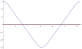
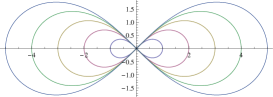
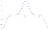
Figure 3. The shrinking figure eight (middle), along with plots of its curvature (left) and second arc length derivative of curvature (right). The horizontal axis represents the $u$ variable and the vertical axis represents $\kappa(u)$ and $\kappa_{ss}(u)$ in the left and right figures respectively.

7. Curves evolving by rotation

A family of curves $\gamma:\SS\times[0,T)\rightarrow\mathbb{R}^{2}$ evolving purely by rotation satisfies

(16) $$-\kappa_{ss}\equiv 2S(t)\left\langle\gamma_{s},\gamma\right\rangle\mbox{.}$$

In particular, if (16) is satisfied for a curve $\gamma_{0}$, then the curve diffusion flow evolving from that curve evolves purely by translation. We call the solution $\gamma_{t}$ a rotator.

Rotators have been conjectured to exist for the curve shortening flow for some time, with a specific conjecture in Altschuler [A91]. A rigorous classification of these has only recently appeared in the literature however [H12]. In this section we prove some classification results for rotators. Our method is to multiply (16) by the curvature and integrate.

Proposition 14.

Let $\gamma:\SS\rightarrow\mathbb{R}^{2}$ be a smooth closed rotator. Then $\gamma$ is a standard round circle.

Proof: The unit normal vector satisfies

$$0=\frac{1}{2}\partial_{s}|\nu|^{2}=\left\langle\nu,\nu_{s}\right\rangle\,.$$

Using the Frenet-Serret frame equations,

$$\int_{\gamma}\kappa_{s}^{2}\,d\ell=-\int_{\gamma}\kappa\,\kappa_{ss}\,d\ell=-2S\int_{\gamma}\left\langle k\gamma_{s},\gamma\right\rangle\,d\ell=2S\int_{\gamma}\left\langle\nu_{s},\gamma\right\rangle\,d\ell=-2S\int_{\gamma}\left\langle\nu,\gamma_{s}\right\rangle\,d\ell=0\,,$$

irrespective of $S$. The curvature of $\gamma$ is therefore constant and its image must be a round circle. $\Box$

Let us now turn to open curves.

Proposition 15.

Suppose $\gamma:\mathbb{R}\rightarrow\mathbb{R}^{2}$ is a smooth open rotator satisfying

(17) $$\lim_{i\rightarrow\infty}\Big{[}\big{(}\kappa(p_{i})\kappa_{s}(p_{i})-2S\left\langle\nu(p_{i}),\gamma(p_{i})\right\rangle\big{)}-\big{(}\kappa(q_{i})\kappa_{s}(q_{i})-2S\left\langle\nu(q_{i}),\gamma(q_{i})\right\rangle\Big{)}\Big{]}=0$$

for arbitrary sequences $\{p_{i}\}$ and $\{q_{i}\}$ asymptotic to $-\infty$ and $+\infty$ respectively. Then $\gamma(\mathbb{R})$ is a straight line.

Proof: Integrate (16) against $\kappa$ to find

$$\int_{p_{i}}^{q_{i}}\kappa_{s}^{2}d\ell =-\int_{p_{i}}^{q_{i}}\kappa\kappa_{ss}\,d\ell+\kappa\kappa_{s}\big{|}_{p_{i}}^{q_{i}}$$

$$=-2S\int_{p_{i}}^{q_{i}}\left\langle\nu_{s},\gamma\right\rangle\,d\ell+\kappa\kappa_{s}\big{|}_{p_{i}}^{q_{i}}$$

$$=\Big{[}-2S\left\langle\nu,\gamma\right\rangle+\kappa\kappa_{s}\Big{]}_{p_{i}}^{q_{i}}\,.$$

Taking $i\rightarrow\infty$ yields the result. $\Box$

Remark: The result of Proposition 15 is false without condition (17), for the same reason that Proposition 11 is false without condition (12).

As with translators earlier, we may convert (17) from a pointwise decay condition on the curvature to a natural growth condition on $\kappa$ in $L^{2}$ and $S\left\langle\nu,\gamma\right\rangle$ in $L^{1}$.

Proposition 16.

Suppose $\gamma:\mathbb{R}\rightarrow\mathbb{R}^{2}$ is a smooth open proper rotator satisfying

(18) $$\lim_{\rho\rightarrow\infty}\bigg{(}\frac{1}{\rho^{2}}\int_{\gamma^{-1}(B_{\rho}(0))}\kappa^{2}\,d\ell+\frac{|S|}{\rho}\int_{\gamma^{-1}(B_{2\rho}(0))}\big{|}\left\langle\nu,\gamma\right\rangle\big{|}\,d\ell\bigg{)}=0\,,$$

where $B_{\rho}(0)$ denotes the closed ball of radius $\rho$ centred at the origin. Then $\gamma(\mathbb{R})$ is a straight line.

Proof: Let $\eta_{\rho}=\tilde{\eta}_{\rho}\circ\gamma$ be the cutoff function used in the proof of Proposition 12. We compute

$$\int_{\gamma^{-1}(B_{\rho}(0))}\kappa_{s}^{2}\,\eta^{4}\,d\ell =-\int_{\gamma^{-1}(B_{\rho}(0))}\kappa\kappa_{ss}\,\eta^{4}\,d\ell-4\int_{\gamma^{-1}(B_{\rho}(0))}\kappa\kappa_{s}\,\eta_{s}\,\eta^{3}\,d\ell$$

$$=2S\int_{\gamma^{-1}(B_{\rho}(0))}\left\langle\nu_{s},\gamma\right\rangle\,\eta^{4}\,d\ell-4\int_{\gamma^{-1}(B_{\rho}(0))}\kappa\kappa_{s}\,\eta_{s}\,\eta^{3}\,d\ell$$

$$=-8S\int_{\gamma^{-1}(B_{\rho}(0))}\left\langle\nu,\gamma\right\rangle\,\eta_{s}\,\eta^{3}\,d\ell-4\int_{\gamma^{-1}(B_{\rho}(0))}\kappa\kappa_{s}\,\eta_{s}\,\eta^{3}\,d\ell$$

$$\leq\varepsilon\int_{\gamma^{-1}(B_{\rho}(0))}\kappa_{s}^{2}\,\eta^{4}\,d\ell+8|S|\int_{\gamma^{-1}(B_{\rho}(0))}\big{|}\left\langle\nu,\gamma\right\rangle\big{|}\,|\eta_{s}|\,\eta^{3}\,d\ell$$

$$\qquad+\frac{4}{\varepsilon}\int_{\gamma^{-1}(B_{\rho}(0))}\kappa^{2}\,\eta_{s}^{2}\,\eta^{2}\,d\ell\,,$$

for any $\varepsilon>0$. Choosing $\varepsilon=\frac{1}{4}$ and absorbing the first term on the left, we find

$$\int_{\gamma^{-1}(B_{\rho}(0))}\kappa_{s}^{2}\,\eta^{4}\,d\ell\leq\frac{c}{\rho^{2}}\int_{\gamma^{-1}(B_{2\rho}(0))}\kappa^{2}\,d\ell+\frac{c|S|}{\rho}\int_{\gamma^{-1}(B_{2\rho}(0))}\big{|}\left\langle\nu,\gamma\right\rangle\big{|}\,d\ell\,.$$

Taking $\rho\rightarrow\infty$ in this estimate yields $\kappa_{s}=0$ and hence the result. $\Box$