11-colored knot diagram with five colors

Abstract.

We prove that any $11$-colorable knot is presented by an $11$-colored diagram where exactly five colors of eleven are assigned to the arcs. The number five is the minimum for all non-trivially $11$-colored diagrams of the knot. We also prove a similar result for any $11$-colorable ribbon $2$-knot.

1. Introduction

The $n$-colorability introduced by Fox [3] is one of the elementary notion in knot theory, and its properties have been studied in many papers. In $1999$, Harary and Kauffman [5] defined a kind of minimal invariant, ${\rm C}_{n}(K)$, of an $n$-colorable knot $K$. It is essential to consider the case that $n$ is an odd prime; in fact, for composite $n$, it is reduced to the cases of odd prime factors of $n$. In this case, we can define a modified version by restricting “effective” $n$-colorings (cf. [6, 12]).

Let $p$ be an odd prime. A non-trivial $p$-coloring $C$ of a knot diagram $D$ is regarded as a non-constant map

$$C:\mbox{\{arcs of $D$\}}\rightarrow{\mathbb{Z}}/p{\mathbb{Z}}=\{0,1,\dots,p-1\}$$

with a certain condition. For a $p$-colorable knot $K$, the number ${\rm C}_{p}(K)$ is defined to be the minimum number of $\#{\rm Im}(C)$ for all non-trivially $p$-colored diagrams $(D,C)$ of $K$. This number has been studied in some papers [2, 4, 7, 8, 10, 11, 13, 15, 17]. In particular, it is shown in [11] that

$${\rm C}_{p}(K)\geq\lfloor\log_{2}p\rfloor+2$$

for any $p$-colorable knot $K$, and the equality holds for $p=3,5,7$ [13, 17].

For $p=11$, we have ${\rm C}_{11}(K)\geq 5$ by the above inequality or [10, Theorem 2.4]. On the other hand, it is proved in [2] that ${\rm C}_{11}(K)\leq 6$. If an $11$-colored diagram $(D,C)$ satisfies $\#{\rm Im}(C)=5$, then there are two possibilities

$${\rm Im}(C)=\{1,4,6,7,8\},\ \{0,4,6,7,8\}$$

up to isomorphisms induced by affine maps of ${\mathbb{Z}}/11{\mathbb{Z}}$. This split phenomenon is quite different from the cases $p=3,5,7$.

Theorem 1.1.

Any $11$-colorable knot $K$ satisfies the following.

• There is an $11$-colored diagram $(D_{1},C_{1})$ of $K$ with ${\rm Im}(C_{1})=\{1,4,6,7,8\}$.

• There is an $11$-colored diagram $(D_{2},C_{2})$ of $K$ with ${\rm Im}(C_{2})=\{0,4,6,7,8\}$.

We remark that these two sets are common $11$-minimal sufficient sets of colors but not universal ones in the sense of [4]. By Theorem 1.1, we have the following immediately.

Corollary 1.2.

Any $11$-colorable knot $K$ satisfies ${\rm C}_{11}(K)=5$. $\Box$

This paper is organized as follows. In Section 2, we review the palette graph associated with a subset of ${\mathbb{Z}}/p{\mathbb{Z}}$ and its fundamental properties. In Section 3, we prove Theorem 1.1(i). The starting point of the proof is a modified version of the theorem in [2]: For any $11$-colorable knot $K$, there is an $11$-colored diagram $(D,C)$ of $K$ with ${\rm Im}(C)=\{0,1,4,6,7,8\}$. By applying Reidemeister moves to $(D,C)$ suitably, we remove the color $0$ from the diagram. Sections 4–6 are devoted to proving Theorem 1.1(ii). We first remove the color $1$ from $(D,C)$ as above by allowing the birth of new colors $3$ and $10$ in Section 4, and then remove the colors $10$ and $3$ in Sections 5 and 6, respectively. In the last section, we prove a similar result for an $11$-colorable ribbon $2$-knot.

2. Preliminaries

Throughout this section, $p$ denotes an odd prime.

Definition 2.1.

Let $S$ be a subset of ${\mathbb{Z}}/p{\mathbb{Z}}$. The palette graph $G(S)$ of $S$ is a simple graph such that

• the vertex set of $G(S)$ is $S$, and

• two vertices $a$ and $b\in S$ are connected by an edge if and only if $\frac{a+b}{2}\in S$.

By assigning $\frac{a+b}{2}$ to every edge joining $a$ and $b$, we regard $G(S)$ as a labeled graph. Such an edge is denoted by $\{a|\frac{a+b}{2}|b\}$.

Definition 2.2.

For two subsets $S$ and $S^{\prime}\subset{\mathbb{Z}}/p{\mathbb{Z}}$, the palette graphs $G(S)$ and $G(S^{\prime})$ are said to be isomorphic if there is a bijection $f:S\rightarrow S^{\prime}$ such that $\frac{a+b}{2}\in S$ if and only if $\frac{f(a)+f(b)}{2}\in S^{\prime}$. We denote it by $G(S)\cong G(S^{\prime})$.

Lemma 2.3.

If $S\subset S^{\prime}\subset{\mathbb{Z}}/p{\mathbb{Z}}$, then $G(S)$ is a subgraph of $G(S^{\prime})$, which is obtained from $G(S^{\prime})$ by deleting the vertices in $S^{\prime}\setminus S$ and the edges whose labels belong to $S^{\prime}\setminus S$.

Proof.

This follows from definition immediately. ∎

Theorem 2.4 ([11]).

If the palette graph $G(S)$ is connected with $\#S>1$, then we have $\#S\geq\lfloor\log_{2}p\rfloor+2$. $\Box$

Lemma 2.5.

Let $S$ be a subset of ${\mathbb{Z}}/p{\mathbb{Z}}$ such that $G(S)$ is connected with $\#S=\lfloor\log_{2}p\rfloor+2$. Put $U=\{S^{\prime}\subset{\mathbb{Z}}/p{\mathbb{Z}}|G(S^{\prime})\cong G(S)\}$. Then we have $\#U=p(p-1)$.

Proof.

Let $T$ be a maximal tree of $G(S)$. Let $v_{1},v_{2},\dots,v_{k}$ be the vertices of $T$, and $e_{1},e_{2},\dots,e_{k-1}$ the edges of $T$, where $k=\#S=\lfloor\log_{2}p\rfloor+2$. Let $A=(a_{ij})$ be the $(k-1)\times k$ matrix with ${\mathbb{Z}}$-entries defined by

$$a_{ij}=\left\{\begin{array}[]{rl}1&\mbox{($e_{i}$ is incident to $v_{j}$)},\\ -2&\mbox{(the label of $e_{i}$ is $v_{j}$)},\\ 0&\mbox{(otherwise)}.\end{array}\right.$$

Let $A^{\prime}$ be the $(k-1)\times(k-1)$ matrix obtained from $A$ by deleting the $k$th column. It is known in [11] that

• ${\rm det}(A^{\prime})$ is odd,

• $|{\rm det}(A^{\prime})|<2^{k-1}$, and

• ${\rm det}(A^{\prime})$ is divisible by $p$.

Since $2^{k-2}<p\leq|{\rm det}(A^{\prime})|<2^{k-1}$, we have $|{\rm det}(A^{\prime})|=p$. This implies that the corank of $A$ with ${\mathbb{Z}}/p{\mathbb{Z}}$-entries is exactly equal to $2$.

Let $V=\{{\mbox{\boldmath$x$}}|A{\mbox{\boldmath$x$}}\equiv{\mbox{\boldmath$0$}}\mbox{ (mod $p$)}\}$ denote the solution space. By the above argument, we have

$$V=\{\lambda\cdot{}^{\rm t}(v_{1},v_{2},\dots,v_{k})+\mu\cdot{}^{\rm t}(1,1,\dots,1)|\lambda,\mu\in{\mathbb{Z}}/p{\mathbb{Z}}\}.$$

Since the elements of $U$ are identified with the vectors of $V$ whose entries are all distinct. Such a vector is obtained by the condition $\lambda\not\equiv 0$ (mod $p$). Therefore, we have $\#U=p(p-1)$. ∎

Theorem 2.6.

Let $S$ and $S^{\prime}$ be subsets of ${\mathbb{Z}}/p{\mathbb{Z}}$. Suppose that $G(S)$ and $G(S^{\prime})$ are connected with $\#S=\#S^{\prime}=\lfloor\log_{2}p\rfloor+2$. Then the following are equivalent.

• The palette graphs $G(S)$ and $G(S^{\prime})$ are isomorphic.

• There exist $\alpha\not\equiv 0$ and $\beta\in{\mathbb{Z}}/p{\mathbb{Z}}$ such that the affine map $f(x)=\alpha x+\beta$ satisfies $f(S)=S^{\prime}$.

Proof.

(ii)$\Rightarrow$(i). Since $\alpha\not\equiv 0$ (mod $p$), $f:S\rightarrow S^{\prime}$ is a bijection. Furthermore, $\frac{a+b}{2}\in S$ holds if and only if $f(\frac{a+b}{2})=\frac{f(a)+f(b)}{2}\in f(S)=S^{\prime}$ holds.

(i)$\Rightarrow$(ii). By the above argument, we have

$$U\supset\{f(S)|f(x)=\alpha x+\beta,\alpha\not\equiv 0,\beta\in{\mathbb{Z}}/p{\mathbb{Z}}\},$$

where $U$ is the set in Lemma 2.5. Since these two sets have the same number of elements by Lemma 2.5, they are the same set. ∎

Let $D$ be a diagram of a knot $K$. We regard $D$ as a disjoint union of arcs whose endpoints are under-crossings. Fox [3] introduced the notion of $p$-colorings: A map $C:\{\mbox{arcs of $D$}\}\rightarrow{\mathbb{Z}}/p{\mathbb{Z}}$ is a $p$-coloring if $a+b\equiv 2c$ (mod $p$) holds at every crossing, where $a$ and $b$ are the elements assigned to the under-arcs by $C$, and $c$ is the one to the over-arc. The triple $\{a|c|b\}$ is called the color of the crossing. The assigned element of an arc of $D$ is called the color of the arc. If the color of an arc is $a$, then the arc is called an $a$-arc.

In a $p$-colored diagram $(D,C)$, the crossing of color $\{a|a|a\}$ is called trivial, and otherwise non-trivial. If $C$ is a constant map, it is called a trivial $p$-coloring, and otherwise, non-trivial. In other words, a $p$-coloring $C$ is non-trivial if and only if $\#{\rm Im}(C)>1$. If a knot $K$ admits a non-trivially $p$-colored diagram $(D,C)$, $K$ is called $p$-colorable.

For a $p$-colorable knot $K$, we denote by ${\rm C}_{p}(K)$ the minimum number of $\#{\rm Im}(C)$ for all non-trivially $p$-colored diagram $(D,C)$ of $K$ [5]. For the study of this number, it is helpful to use the palette graph $G({\rm Im}(C))$ of the image ${\rm Im}(C)\subset{\mathbb{Z}}/p{\mathbb{Z}}$ in the following sense.

Lemma 2.7.

If $\{a|c|b\}$ is a non-trivial color of a crossing of a $p$-colored diagram $(D,C)$, then the palette graph $G({\rm Im}(C))$ has an edge $\{a|c|b\}$.

Proof.

Since $a+b\equiv 2c$ (mod $p$) holds, the lemma follows by definition. ∎

Lemma 2.8.

The palette graph $G({\rm Im}(C))$ of a $p$-colored diagram $(D,C)$ of a knot is connected.

Proof.

Let $a$ and $b$ be vertices of $G({\rm Im}(C))$. By definition, we have an $a$-arc and a $b$-arc of $D$. Since $D$ is a diagram of a knot (not a link), we can walk along $D$ from the $a$-arc to the $b$-arc. Let $\{a_{i}|c_{i}|a_{i+1}\}$ $(1\leq i\leq k-1)$ be the colors of non-trivial under-crossings on the path such that $a_{1}=a$ and $a_{k}=b$. Then the vertices $a$ and $b$ in the palette graph are connected by a sequence of edges $\{a_{i}|c_{i}|a_{i+1}\}$ $(1\leq i\leq k-1)$. ∎

Theorem 2.9 ([11]).

Any non-trivial $p$-colored diagram $(D,C)$ of a knot satisfies $\#{\rm Im}(C)\geq\lfloor\log_{2}p\rfloor+2$. Therefore, we have ${\rm C}_{p}(K)\geq\lfloor\log_{2}p\rfloor+2$ for any $p$-colorable knot $K$.

Proof.

This follows from Theorem 2.4 and Lemma 2.8. ∎

Lemma 2.10.

Let $(D,C)$ be a non-trivially $p$-colored diagram of a knot $K$, and $f:{\mathbb{Z}}/p{\mathbb{Z}}\rightarrow{\mathbb{Z}}/p{\mathbb{Z}}$ an affine map defined by $f(x)=\alpha x+\beta$ with $\alpha\not\equiv 0$ and $\beta\in{\mathbb{Z}}/p{\mathbb{Z}}$. Then there is a non-trivially $p$-colored diagram $(D,C^{\prime})$ of $K$ such that ${\rm Im}(C^{\prime})=f({\rm Im}(C))$.

Proof.

It is easy to see that the composition $C^{\prime}=f\circ C$ is also a non-trivial $p$-coloring of $D$. ∎

Now, we consider the case $p=11$. By Theorem 2.4, if the palette graph $G(S)$ of a subset $S\subset{\mathbb{Z}}/11{\mathbb{Z}}$ is connected with $\#S>1$, then $\#S\geq 5$.

Theorem 2.11 ([4, Theorem 12]).

Let $S$ be a subset of ${\mathbb{Z}}/11{\mathbb{Z}}$. If the palette graph $G(S)$ is connected with $\#S=5$, then $G(S)$ is isomorphic to $G(\{1,4,6,7,8\})$ or $G(\{0,4,6,7,8\})$ as shown in Figure 1. $\Box$

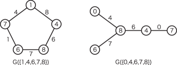
Figure 1.

By Theorem 2.9 or [10, Theorem 2.4], we have ${\rm C}_{11}(K)\geq 5$. The following theorem implies that ${\rm C}_{11}(K)=5$ or $6$.

Theorem 2.12 ([2]).

For any $11$-colorable knot $K$, there is a non-trivially $11$-colored diagram $(D,C)$ of $K$ with ${\rm Im}(C)\subset\{0,1,4,6,7,8\}$. $\Box$

Figure 2 shows the palette graph $G(\{0,1,4,6,7,8\})$. By Lemma 2.3, the two graphs in Theorem 2.11 are obtained from this graph by deleting the vertex $a$ and the edges labeled $a$ for $a=0,1$, respectively.

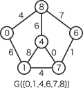
Figure 2.

It is useful for our argument to modify Theorem 2.12 slightly as follows.

Lemma 2.13.

For any $11$-colorable knot $K$, there is an $11$-colored diagram $(D,C)$ of $K$ with ${\rm Im}(C)=\{0,1,4,6,7,8\}$.

Proof.

We may assume that $(D,C)$ satisfies Theorem 2.12; that is, it is a non-trivially $11$-colored diagram with ${\rm Im}(C)\subset\{0,1,4,6,7,8\}$. We remark that $\#{\rm Im}(C)\geq 5$ by Theorem 2.9.

$4,6,7\in{\rm Im}(C)$. Assume that $4\not\in{\rm Im}(C)$. It follows that ${\rm Im}(C)=\{0,1,6,7,8\}$. The palette graph $G({\rm Im}(C))$ is as shown in the left of Figure 3 by Lemma 2.3, which contradicts to the connectivity in Lemma 2.8. We can also prove $6,7\in{\rm Im}(C)$ by a similar argument. See the center and right of the figure.

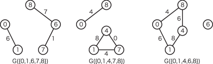
Figure 3.

$0\in{\rm Im}(C)$. Assume that $0\not\in{\rm Im}(C)$. It follows that ${\rm Im}(C)=\{1,4,6,7,8\}$ and its palette graph is as shown in the left of Figure 1. Then we see that $(D,C)$ has a crossing of color $\{6|1|7\}$ or $\{1|8|4\}$. In fact, if we delete the corresponding edges both, the resulting graph becomes disconnected. By deforming the diagram near these crossings as shown in Figure 4, we can produce a $0$-arc. We replace the original diagram with the new one as $(D,C)$.

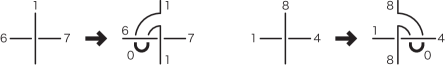
Figure 4.

$1\in{\rm Im}(C)$. Assume that $1\not\in{\rm Im}(C)$. Then we have ${\rm Im}(C)=\{0,4,6,7,8\}$ and its palette graph is as shown the right of Figure 1. Since $(D,C)$ must have a crossing of color $\{0|4|8\}$ by a similar reason to the above case, we deform the diagram near the crossing to make a $1$-arc. See Figure 5.

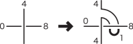
Figure 5.

$8\in{\rm Im}(C)$. Assume that $8\not\in{\rm Im}(C)$. Then we have ${\rm Im}(C)=\{0,1,4,6,7\}$ and its palette graph is as shown in the left of Figure 6. We remark that the map $f:{\mathbb{Z}}/11{\mathbb{Z}}\rightarrow{\mathbb{Z}}/11{\mathbb{Z}}$ defined by $f(x)=7x+6$ induces the isomorphism between $G(\{0,4,6,7,8\})$ and $G(\{0,1,4,6,7\})$. The existence of such a map is guaranteed by Theorem 2.6. Since $(D,C)$ has a crossing of color $\{4|0|7\}$, we deform the diagram near the crossing as shown in the right of the figure so that we obtain an $8$-arc. ∎

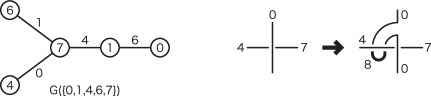
Figure 6.

3. Proof of Theorem 1.1(i)

Lemma 3.1.

For any $11$-colorable knot $K$, there is an $11$-colored diagram $(D,C)$ of $K$ such that

• ${\rm Im}(C)=\{0,1,4,6,7,8\}$, and

• there is no crossing of color $\{*|0|*\}$.

Proof.

We may assume that $(D,C)$ satisfies Lemma 2.13. There are two types of crossings of $(D,C)$ whose over-arc is a $0$-arc; that is, $\{0|0|0\}$ and $\{4|0|7\}$. In fact, in the palette graph $G(\{0,1,4,6,7,8\})$, the only edge labeled $0$ connects $4$ and $7$.

First, we assume that $(D,C)$ has crossings of color $\{4|0|7\}$. By deforming the diagram near the crossings as shown in Figure 7, we can eliminate all the crossings of color $\{4|0|7\}$. We remark that the set of colors which are appeared in the diagram does not change.

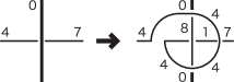
Figure 7.

Next, we assume that $(D,C)$ has a crossing of color $\{0|0|0\}$, say $x$. Walking along the diagram from $x$, let $y$ be the non-trivial crossing which we meet first. If there are crossings of color $\{0|0|0\}$ between $x$ and $y$, we replace the original $x$ with the nearest one to $y$. Therefore, we may assume that there is no crossing between $x$ and $y$.

There are two cases with respect to the color of $y$. In fact, in the palette graph $G(\{0,1,4,6,7,8\})$, there are two edges incident to the vertex $0$, which implies that the color of $y$ is $\{0|6|1\}$ or $\{0|4|8\}$. In each case, we deform the diagram $(D,C)$ near $x$ and $y$ as shown in Figure 8, so that the number of crossings of $\{0|0|0\}$ is decreased. By repeating this process, we obtain a diagram with no crossing of $\{0|0|0\}$ finally. ∎

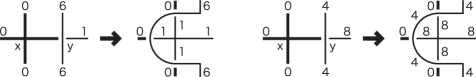
Figure 8.

Proof of Theorem 1.1(i)..

We may assume that $(D,C)$ satisfies Lemma 3.1. If there is a $0$-arc, it is not an over-arc of any crossing, and its endpoints are the under-crossings of color $\{0|4|8\}$ or $\{0|6|1\}$. In fact, there are two edges incident to the vertex $0$ in $G(\{1,4,6,7,8\})$. We have three cases with respect to the colors of the crossings of the endpoints of a $0$-arc;

• $\{0|4|8\}$ and $\{0|6|1\}$,

• $\{0|4|8\}$ both, and

• $\{0|6|1\}$ both.

For the case (i), we deform the $6$-arc over the crossing of $\{0|4|8\}$ to eliminate the $0$-arc. See the top of Figure 9. For the case (ii), we deform one of the crossings of color $\{0|4|8\}$ as shown in the figure so that we reduce this case to (i). Similarly, for the case (iii), we deform one of the crossings of color $\{0|6|1\}$ as shown in the figure so that we reduce this case to (i). See the bottom of the figure. ∎

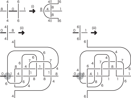
Figure 9.

Corollary 3.2.

For any $11$-colorable knot $K$ and $a\not\equiv b\in{\mathbb{Z}}/11{\mathbb{Z}}$, there is an $11$-colored diagram $(D,C)$ of $K$ with

$${\rm Im}(C)=\{a,b,3a+9b,6a+6b,10a+2b\}.$$

Proof.

Let $f:{\mathbb{Z}}/11{\mathbb{Z}}\rightarrow{\mathbb{Z}}/11{\mathbb{Z}}$ be the affine map defined by $f(x)=4(b-a)(x-1)+a$. Since the map $f$ satisfies

$$f(1)=a,\ f(4)=b,\ f(6)=3a+9b,\ f(7)=10a+2b,\ f(8)=6a+6b,$$

we have the conclusion by Lemma 2.10 and Theorem 1.1(i). ∎

4. Proof of Theorem 1.1(ii)–Part I

Lemma 4.1.

For any $11$-colorable knot $K$, there is an $11$-colored diagram $(D,C)$ of $K$ such that

• ${\rm Im}(C)=\{0,1,4,6,7,8\}$, and

• there is no crossing of color $\{6|6|6\}$.

Proof.

We may assume that $(D,C)$ satisfies Lemma 2.13. Assume that $(D,C)$ has a crossing of color $\{6|6|6\}$, say $x$. Walking along the diagram from $x$, let $y$ be the first non-trivial under-crossing. If there are crossings of color $\{6|6|6\}$ between $x$ and $y$, then we replace the original $x$ with the nearest one to $y$. Then we have the following:

• There is no crossing of $\{6|6|6\}$ between $x$ and $y$ by assumption.

• Every crossing between $x$ and $y$ is of color $\{0|6|1\}$ or $\{4|6|8\}$; for there are exactly two edges labeled $6$ in the palette graph $G(\{0,1,4,6,7,8\})$.

• The color of $y$ is $\{6|1|7\}$ or $\{6|7|8\}$; for there are exactly two edges incident to the vertex $6$ in the palette graph, which are labeled $1$ and $7$, respectively.

Assume that there are crossings between $x$ and $y$. Let $z$ be the nearest crossing to $x$ among them. We deform the diagram near $x$ and $z$ as shown in the upper row of Figure 10, so that the number of crossings between $x$ and $y$ is decreased. By repeating this process, we may assume that there is no crossing between $x$ and $y$. Then we deform the diagram near $x$ and $y$ as shown in the lower row of the figure to eliminate the color $\{6|6|6\}$. By repeating this process, we obtain a diagram with no crossing of $\{6|6|6\}$ finally. ∎

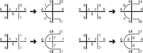
Figure 10.

Lemma 4.2.

For any $11$-colorable knot $K$, there is an $11$-colored diagram $(D,C)$ of $K$ such that

• ${\rm Im}(C)=\{0,1,4,6,7,8\}$, and

• there is no crossing of color $\{1|1|1\}$ or $\{6|6|6\}$.

Proof.

We may assume that $(D,C)$ satisfies Lemma 4.1. Assume that $(D,C)$ has a crossing of color $\{1|1|1\}$, say $x$. Walking along the diagram from $x$, let $y$ be the first non-trivial crossing. If there are crossing of $\{1|1|1\}$ between $x$ and $y$, then we replace the original $x$ with the nearest one to $y$.

In the palette graph $G(\{0,1,4,6,7,8\})$, there are exactly three edges incident to the vertex $1$ whose labels are $4$, $6$, and $8$, and there is only one edge whose label is $1$. Therefore, the color of the crossing $y$ is $\{1|4|7\}$, $\{1|6|0\}$, $\{1|8|4\}$, or $\{6|1|7\}$.

We deform the diagram near $x$ and $y$ as shown in Figure 11 so that the number of crossings of color $\{1|1|1\}$ is decreased. By repeating this process, we obtain a diagram with no crossing of $\{1|1|1\}$. ∎

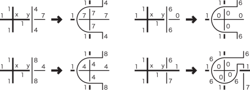
Figure 11.

Lemma 4.3.

For any $11$-colorable knot $K$, there is a non-trivially $11$-colored diagram $(D,C)$ of $K$ such that

• ${\rm Im}(C)=\{0,1,4,6,7,8\}$, and

• there is no crossing of color $\{*|1|*\}$ or $\{6|6|6\}$.

Proof.

We may assume that $(D,C)$ satisfies Lemma 4.2. Assume that $(D,C)$ has a crossing of color $\{*|1|*\}$. Since there is only one edge labeled $1$ in the palette graph $G(\{0,1,4,6,7,8\})$, the color of the corresponding crossing is $\{6|1|7\}$.

There is a $4$-arc in $(D,C)$. We will pull the $4$-arc toward each crossing of $\{6|1|7\}$. In the process, we can assume that the $4$-arc crosses over several arcs whose colors are $0,1,4,7,8$ missing $6$. In fact, since there is no crossing of $\{6|6|6\}$, the set of $6$-arcs is a disjoint union of intervals in the plane, and the complement in the plane is connected. When the $4$-arc crosses over an $a$-arc for $a=0,1,4,7,8$, we have a pair of new crossings of color

$$\{a|4|8-a\}=\{0|4|8\},\ \{1|4|7\},\ \{4|4|4\},\ \{7|4|1\},\ \{8|4|0\},$$

respectively. See the left of Figure 12. We remark that any vertex of the palette graph $G(\{0,1,4,6,7,8\})$ other than $6$ is $4$ itself or incident to an edge labeled $4$.

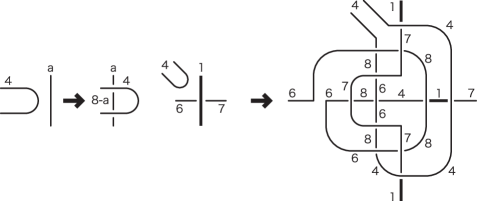
Figure 12.

By deforming the diagram near every crossing of $\{6|1|7\}$ with a $4$-arc as shown in the right of the figure, we obtain a diagram with no crossing of $\{6|1|7\}$. Then the arcs in the obtained diagram are colored by $0,1,4,6,7,8$ and there is no crossing of $\{*|1|*\}$ or $\{6|6|6\}$. ∎

Lemma 4.4.

For any $11$-colorable knot $K$, there is an $11$-colored diagram $(D,C)$ of $K$ such that

• ${\rm Im}(C)=\{0,3,4,6,7,8,10\}$,

• there is no crossing of color $\{6|6|6\}$, and

• if $\{a|b|c\}$ is the color of a crossing and at least one of $a,b,c$ is $3$ or $10$, then it is one of

  $$\{0|3|6\},\ \{0|7|3\},\ \{3|0|8\},\ \{4|7|10\},\ \{7|3|10\},\ \{3|3|3\}.$$

Proof.

We may assume that $(D,C)$ satisfies Lemma 4.3. Since there are three edges incident to the vertex $1$ in the palette graph $G(\{0,1,4,6,7,8\})$, every crossing with a $1$-arc is of color $\{1|4|7\}$, $\{1|6|0\}$, or $\{1|8|4\}$. If there is a crossing of $\{1|8|4\}$, we deform the $4$-arc near the crossing as shown in Figure 13 to replace the crossing with the one of color $\{1|4|7\}$. Therefore, we may assume that there is no crossing of $\{1|8|4\}$.

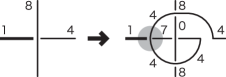
Figure 13.

There is a $0$-arc in $(D,C)$. We will pull the $0$-arc toward each crossing of $\{1|4|7\}$. In the process, we can assume that the $0$-arc crosses over several $a$-arcs for $a\in\{0,1,4,7,8\}$ missing $6$ by the same reason in the proof of Lemma 4.3; that is, there is no crossing of $\{6|6|6\}$. When the $0$-arc crosses over an $a$-arc, we have a pair of new crossings of color

$$\{a|0|-a\}=\{0|0|0\},\ \{1|0|10\},\ \{4|0|7\},\ \{7|0|4\},\ \{8|0|3\},$$

respectively. We remark that the new colors $3$ and $10$ appear at the crossings of $\{1|0|10\}$ and $\{3|0|8\}$. See Figure 14.

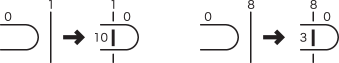
Figure 14.

By deforming the diagram near every crossing of $\{1|4|7\}$ with a $0$-arc as shown in Figure 15, we remove all the crossings of $\{1|4|7\}$ and produce the color $10$ at the crossings of $\{1|0|10\}$ and $\{4|7|10\}$.

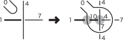
Figure 15.

There is a $7$-arc in $(D,C)$. We will pull the $7$-arc toward each $0$-arc. In the process, we can assume that the $7$-arc crosses over several $a$-arcs for $a\in\{0,3,4,6,7,8,10\}$ missing $1$; for there is no crossing of $\{1|1|1\}$. Then we have a pair of new crossings of

$$\{a|7|3-a\}=\{0|7|3\},\ \{3|7|0\},\ \{4|7|10\},\ \{6|7|8\},\ \{7|7|7\},\ \{8|7|6\},\ \{10|7|4\},$$

respectively. We remark that the colors $3$ and $10$ appear at the crossings of $\{0|7|3\}$ and $\{4|7|10\}$.

Now, every crossing with a $1$-arc is of color $\{1|6|0\}$ or $\{1|0|10\}$. The endpoints of every $1$-arc are under-crossings of color

• $\{1|6|0\}$ both,

• $\{1|0|10\}$ both, or

• $\{1|0|10\}$ and $\{1|6|0\}$.

For every $1$-arc of type (i), we deform the diagram near the $1$-arc equipped with a $7$-arc into type (ii) as shown in the left of Figure 16. Here, the colors $3$ and $10$ appear at the crossings of $\{0|7|3\}$, $\{7|3|10\}$, $\{0|3|6\}$, $\{3|3|3\}$, and $\{3|0|8\}$.

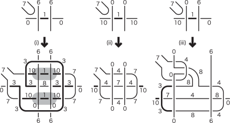
Figure 16.

For every $1$-arc of type (ii) or (iii), we deform the diagram near the $1$-arc with a $7$-arc as shown in the center and right of the figure, so that we can remove all the $1$-arcs from the diagram. We remark that the colors $3$ and $10$ appear at the crossings of $\{4|7|10\}$ for (ii) and $\{3|0|8\}$ and $\{7|3|10\}$ for (iii).

Since the original diagram has a $1$-arc, at least one of deformations (i), (ii), and (iii) must happen. Therefore, the obtained diagram has a $10$-arc. If the diagram has no $3$-arc, the case (ii) must happen. By deforming a neighborhood of a crossing of $\{4|0|7\}$ similarly to Figures 4 and 5, we can make a pair of crossings of $\{0|7|3\}$ so that we have ${\rm Im}(C)=\{0,3,4,6,7,8,10\}$. ∎

We remark that the $11$-colored diagram $(D,C)$ in Lemma 4.4 has no crossing of color $\{3|10|6\}$, $\{6|8|10\}$, or $\{10|10|10\}$. In particular, there is no crossing whose over-arc is colored $10$.

5. Proof of Theorem 1.1(ii)–Part II

Let $G_{1}$ be the graph obtained from the palette graph $G(\{0,4,6,7,8\})$ by adding two vertices $3$ and $10$ and five edges

$$\{0|3|6\},\ \{0|7|3\},\ \{3|0|8\},\ \{4|7|10\},\ \{7|3|10\}.$$

See Figure 17. In other words, $G_{1}$ is obtained from $G(\{0,3,4,5,6,8,10\})$ by deleting the edges $\{3|10|6\}$ and $\{6|8|10\}$.

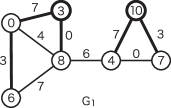
Figure 17.

Assume that $(D,C)$ satisfies Lemma 4.4. If $\{a|c|b\}$ is the non-trivial color of a crossing of $(D,C)$, then the palette graph $G_{1}$ has the corresponding edge $\{a|c|b\}$.

Lemma 5.1.

For any $11$-colorable knot $K$, there is an $11$-colored diagram $(D,C)$ of $K$ such that

• ${\rm Im}(C)=\{0,3,4,6,7,8\}$, and

• there is no crossing of color $\{6|6|6\}$.

Proof.

We may assume that $(D,C)$ satisfies Lemma 4.4. Since the graph $G_{1}$ has no edge whose label is $10$ and $(D,C)$ has no crossing of $\{10|10|10\}$, we see that there is no crossing of color $\{*|10|*\}$.

Since there are two edges incident to the vertex $10$ in $G_{1}$, every crossing with a $10$-arc is of color $\{4|7|10\}$ or $\{7|3|10\}$. If there is a crossing of $\{7|3|10\}$, we deform the $7$-arc near the crossing as shown in the left of Figure 18 to replace the crossing with one of $\{4|7|10\}$. We remark that the crossings of $\{0|7|3\}$ and $\{4|0|7\}$ are also produced. Therefore, we may assume that there is no crossing of $\{7|3|10\}$.

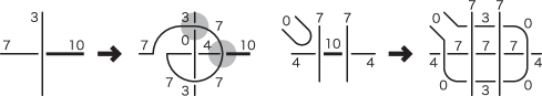
Figure 18.

There is a $0$-arc in $(D,C)$. We will pull the $0$-arc toward each $10$-arc. In the process, we can assume that the $0$-arc crosses over several arcs whose colors are $0,3,4,7,8$ missing $6$ and $10$. In fact, since there is no crossing of color

$$\{3|10|6\},\ \{2|6|10\},\ \{6|8|10\},\ \{6|6|6\},\ \{10|10|10\},$$

the set of $6$- and $10$-arcs is a disjoint union of intervals, and the complement in the plane is connected. When the $0$-arc crosses over an $a$-arc for $a=0,3,4,7,8$, we have a pair of new crossings of color

$$\{a|0|-a\}=\{0|0|0\},\ \{3|0|8\},\ \{4|0|7\},\ \{7|0|4\},\ \{8|0|3\},$$

respectively. We remark that any vertex of $G_{1}$ other than $6$ and $10$ is $0$ itself or incident to an edge labeled $0$.

We deform the diagram near every $10$-arc with a $0$-arc as shown in the right of the figure, so that we remove all the $10$-arcs from the diagram. We remark that the crossings of $\{0|7|3\}$, $\{4|0|7\}$, and $\{7|7|7\}$ are produced. ∎

6. Proof of Theorem 1.1(ii)–Part III

Lemma 6.1.

For any $11$-colorable knot $K$, there is an $11$-colored diagram $(D,C)$ of $K$ such that

• ${\rm Im}(C)=\{0,3,4,6,7,8\}$,

• there is no crossing of color $\{3|3|3\}$, $\{4|4|4\}$, or $\{6|6|6\}$.

Proof.

We may assume that $(D,C)$ satisfies Lemma 5.1 with ${\rm Im}(C)=\{0,3,4,6,7,8\}$. Figure 19 shows the palette graph $G(\{0,3,4,6,7,8\})$, which is obtained from $G_{1}$ by deleting the vertex $10$ and its incident edges $\{4|7|10\}$ and $\{7|3|10\}$.

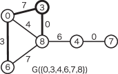
Figure 19.

There is a $0$-arc in $(D,C)$. Similarly to the proof of Lemma 5.1, we can pull the $0$-arc freely without producing new colors. We remark that any vertex of $G(\{0,3,4,6,7,8\})$ other than $6$ is $0$ itself or incident to an edge labeled $0$. Then we deform the diagram near every $3$- or $4$-arc with a $0$-arc as shown in Figure 20 so that there is no crossing of $\{3|3|3\}$ or $\{4|4|4\}$. ∎

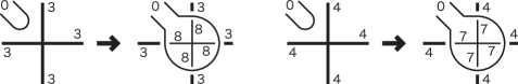
Figure 20.

Lemma 6.2.

For any $11$-colorable knot $K$, there is an $11$-colored diagram $(D,C)$ of $K$ such that

• ${\rm Im}(C)=\{0,3,4,6,7,8\}$,

• there is no crossing of color $\{*|3|*\}$, $\{4|4|4\}$, or $\{6|6|6\}$.

Proof.

We may assume that $(D,C)$ satisfies Lemma 6.1. In the palette graph $G(\{0,3,4,6,7,8\})$, there is only one edge whose label is $3$. Therefore, every crossing whose over-arc is $3$ has the color $\{0|3|6\}$.

There is a $7$-arc in $(D,C)$. We will pull the $7$-arc toward each crossing of $\{0|3|6\}$. Since there is no crossing of $\{4|4|4\}$, we can assume that the $7$-arc crosses over several arcs whose colors are $0,3,6,7,8$ missing $4$. If the $7$-arc crosses an $a$-arc for $a\in\{0,3,6,7,8\}$, then we have a pair of new crossings of color

$$\{a|7|3-a\}=\{0|7|3\},\ \{3|7|0\},\ \{6|7|8\},\ \{7|7|7\},\ \{8|7|6\},$$

respectively. We remark that any vertex of $G(\{0,3,4,6,7,8\})$ other than $4$ is $7$ itself or incident to an edge labeled $7$. We deform the diagram near every crossing of $\{0|3|6\}$ equipped with a $7$-arc as shown in Figure 21 to remove all the crossings of $\{0|3|6\}$. ∎

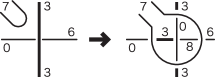
Figure 21.

Proof of Theorem 1.1(ii).

We may assume that $(D,C)$ satisfies Lemma 6.2. Since there are two edges incident to the vertex $3$ in $G(\{0,3,4,6,7,8\})$, every crossing with a $3$-arc is of color $\{3|0|8\}$ or $\{0|7|3\}$. Therefore, the endpoints of every $3$-arc are under-crossings of color

• $\{3|0|8\}$ and $\{0|7|3\}$,

• $\{3|0|8\}$ both, or

• $\{0|7|3\}$ both.

For every $3$-arc of type (i), we deform the diagram near the crossing of $\{0|7|3\}$, which reduces a $3$-arc of type (ii). See the left of Figure 22. Therefore, we may assume that there is no $1$-arc of type (i).

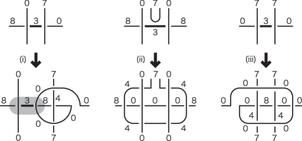
Figure 22.

To remove a $3$-arc of type (ii), We will pull a $7$-arc toward the $3$-arc. Since there is no crossing of $\{4|4|4\}$, the $7$-arc can cross over several arcs whose colors are $0,3,6,7,8$ missing $4$ similarly to the proof of Lemma 6.2. We remark that when the $7$-arc crosses over an $0$- or $3$-arc, then we have a pair of new crossings of color $\{0|7|3\}$. We deform the diagram near every $3$-arc of type (ii) with a $7$-arc to remove all the $3$-arcs of type (ii). See the center of the figure.

Now, since every crossing with a $3$-arc is of color $\{0|7|3\}$, every $3$-arc is of type (iii). We deform the diagram near every $3$-arc of type (iii) with a $7$-arc as shown in the right of the figure so that we obtain a diagram with no $3$-arc. ∎

Corollary 6.3.

For any $11$-colorable knot $K$ and $a\not\equiv b\in{\mathbb{Z}}/11{\mathbb{Z}}$, there is an $11$-colored diagram $(D,C)$ of $K$ with

$${\rm Im}(C)=\{a,b,5a+7b,2a+10b,10a+2b\}.$$

Proof.

Let $f:{\mathbb{Z}}/11{\mathbb{Z}}\rightarrow{\mathbb{Z}}/11{\mathbb{Z}}$ be the affine map defined by $f(x)=3(b-a)x+a$. Since the map $f$ satisfies

$$f(0)=a,\ f(4)=b,\ f(6)=5a+7b,\ f(7)=2a+10b,\ f(8)=10a+2b,$$

we have the conclusion by Lemma 2.10 and Theorem 1.1(ii). ∎

7. $11$-colorable ribbon $2$-knot

A ribbon $2$-knot [3] is a kind of knotted $2$-sphere embedded in ${\mathbb{R}}^{4}$. Such a $2$-knot is presented by a diagram in ${\mathbb{R}}^{3}$ with only double point circles [18], the $n$-colorability is defined similarly to the classical case by assigning an element of ${\mathbb{Z}}/n{\mathbb{Z}}$ to each sheet of the diagram. Refer to [1] for a diagram of a knotted surfaces.

Lemma 7.1.

Let $K$ be an $11$-colorable ribbon $2$-knot. For each set $S=\{1,4,6,7,8\}$ or $\{0,4,6,7,8\}$, there is an $11$-colored diagram of $K$ which satisfies the following.

• Every double point circle has a neighborhood as shown in Figure 23, and all the sheets of the diagram other than the small shaded disks are colored by $S$.

• While the color $2a-b$ of the shaded disk may not belong to $S$, the pair $(a,b)$ must satisfy $2b-a\in S$.

Proof.

Let $A$ be a virtual arc which presents $K$ [16]. Since $K$ is $11$-colorable, so is $A$. Then there is an $11$-colored diagram $(D,C)$ of $A$ with ${\rm Im}(C)=S$ by a similar argument in the proof of Theorems 1.1. The diagram of $K$ associated to $(D,C)$ is the desired one [13, 17]. ∎

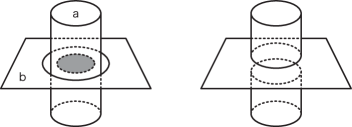
Figure 23.

Theorem 7.2.

Any $11$-colorable ribbon $2$-knot satisfies the following.

• There is an $11$-colored diagram $(D_{1},C_{1})$ of $K$ with ${\rm Im}(C_{1})=\{1,4,6,7,8\}$.

• There is an $11$-colored diagram $(D_{2},C_{2})$ of $K$ with ${\rm Im}(C_{2})=\{0,4,6,7,8\}$.

Proof.

(i) We may assume that $(D,C)$ satisfies Lemma 7.1 for $S=\{1,4,6,7,8\}$. In the left of Figure 23, the shaded disk is colored $2b-a$. The pair $(a,b)$ with $a,b,2b-a\in S$ and $2a-b\not\in S$ is one of the following:

$$(a,b)=(4,1),\ (4,7),\ (1,7),\ (1,6),\ (7,6),\ (7,8),\ (6,8),\ (6,4),\ (8,4),\ (8,1).$$

In fact, each edge $\{x|y|z\}$ in the palette graph $G(S)$ produces such two pairs $(y,x)$ and $(y,z)$.

First, we consider the case $(a,b)=(4,1)$, where the shaded sheet is colored $9$. There is an $8$-sheet in $(D,C)$. We pull the $8$-sheet toward the $9$-sheet without introducing new double points and deform the diagram as shown in the left of Figure 24 to remove the $9$-sheet. We remark that the figure shows a cross-section of the neighborhood of the $9$-sheet. Next, we consider the case $(a,b)=(4,7)$, where the shaded sheet is colored $10$. We deform the horizontal $4$-sheet by surrounding the $10$-sheet, that reduces the case $(a,b)=(4,1)$. See the right of the figure.

Figure 24.

Let $f:{\mathbb{Z}}/11{\mathbb{Z}}\rightarrow{\mathbb{Z}}/11{\mathbb{Z}}$ be the affine map defined by $f(x)=9x+9$. Since we have

$$f(1)=7,\ f(4)=1,\ f(6)=8,\ f(7)=6,\mbox{ and }f(8)=4,$$

the cases $(a,b)=(1,7)$, $(7,6)$, $(6,8)$, and $(8,4)$ are obtained from $(a,b)=(4,1)$ by applying $f$ repeatedly, and the cases $(a,b)=(1,6)$, $(7,8)$, $(6,4)$, and $(8,1)$ are obtained from $(a,b)=(4,7)$ similarly.

(ii) We may assume that $(D,C)$ satisfies Lemma 7.1 for $S=\{0,4,6,7,8\}$. The pair $(a,b)$ with $a,b,2b-a\in S$ and $2a-b\not\in S$ is one of the following:

$$(a,b)=(4,8),\ (7,6),\ (7,8),\ (6,8),\ (6,4),\mbox{ and }(0,7).$$

In fact, each edge $\{x|y|z\}$ in the palette graph $G(S)$ produces such two pairs $(y,x)$ and $(y,z)$ other than $(4,8)$ from $\{0|4|8\}$ and $(0,4)$ from $\{4|0|7\}$.

For the case $(a,b)=(4,8)$, we deform the horizontal $4$-sheet by surrounding the shaded $1$-sheet as shown in the left of Figure 25 so that we can remove the $1$-sheet. The case $(a,b)=(0,7)$ can be similarly proved. See the right of the figure.

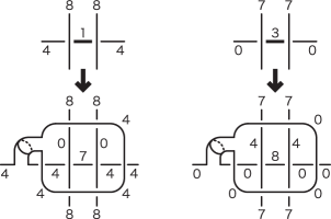
Figure 25.

For the case $(a,b)=(7,6)$, we pull a $0$-sheet and deform the diagram as shown in the left of Figure 26. Then we can remove the $5$-sheet without introducing new colors. For the case $(a,b)=(7,8)$, we first deform the horizontal $7$-sheet by surrounding the shaded $9$-sheet, that reduces to the case $(a,b)=(7,6)$.

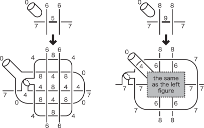
Figure 26.

For the case $(a,b)=(6,8)$, we pull a $7$-sheet and surround the shaded $10$-sheet by the $7$-sheet as shown in the left of Figure 27 so that the color $10$ is removed. For the case $(a,b)=(6,4)$, we pull a $7$-sheet toward the shaded $2$-sheet and deform the horizontal $6$-sheet to surround the $2$-sheet. Then this case reduces to the case $(a,b)=(6,8)$. ∎

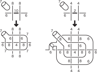
Figure 27.

For a $p$-colorable $2$-knot $K$, we denote by ${\rm C}_{p}(K)$ the minimum number of $\#{\rm Im}(C)$ for all non-trivially $p$-colored diagrams $(D,C)$ of $K$ [17]. Then the following is an immediate consequence of Theorem 7.2.

Corollary 7.3.

Any $11$-colorable ribbon $2$-knot $K$ satisfies ${\rm C}_{11}(K)=5$. $\Box$

The proof of the following is as same as that of Corollaries 3.2 and 6.3.

Corollary 7.4.

For any $11$-colorable ribbon $2$-knot $K$ and $a\not\equiv b\in{\mathbb{Z}}/11{\mathbb{Z}}$, there are $11$-colored diagrams $(D_{1},C_{1})$ and $(D_{2},C_{2})$ of $K$ with

$$\begin{array}[]{l}{\rm Im}(C_{1})=\{a,b,3a+9b,10a+2b,6a+6b\},\ and\\ {\rm Im}(C_{2})=\{a,b,5a+7b,2a+10b,10a+2b\}.\end{array}$$

$\Box$

References

- [1] J. S. Carter and M. Saito, Knotted surfaces and their diagrams, Mathematical Surveys and Monographs, 55. American Mathematical Society, Providence, RI, 1998.
- [2] W. Cheng, X. Jin, and N. Zhao, Any -colorable knot can be colored with at most six colors, J. Knot Theory Ramifications 23 (2014), no. 11, 1450062, 25 pp.
- [3] R. H. Fox, A quick trip through knot theory, 1962 Topology of -manifolds and related topics (Proc. The Univ. of Georgia Institute, 1961) pp. 120–167 Prentice-Hall, Englewood Cliffs, N.J.
- [4] J. Ge, X. Jin, L. H. Kauffman, P. Lopes, and L. Zhang, Minimal sufficient sets of colors and minimum number of colors, available at arXiv: 1501.02421
- [5] F. Harary and L. H. Kauffman, Knots and graphs. I. Arc graphs and colorings, Adv. in Appl. Math. 22 (1999), no. 3, 312–337.
- [6] K. Ichihara and E. Matsudo, A lower bound on minimal number of colors for links, preprint.
- [7] L. H. Kauffman and P. Lopes, On the minimum number of colors for knots, Adv. in Appl. Math. 40 (2008), no. 1, 36–53.
- [8] L. H. Kauffman and P. Lopes, The Teneva game, J. Knot Theory Ramifications 21 (2012), no. 14, 1250125, 17 pp.
- [9] A. Kawauchi, Lectures on knot theory, Monograph in Japanese, 2007, Kyoritsu Shuppan Co. Ltd.
- [10] P. Lopes and J. Matias, Minimum number of Fox colors for small primes, J. Knot Theory Ramifications 21 (2012), no. 3, 1250025, 12 pp.
- [11] T. Nakamura, Y. Nakanishi, and S. Satoh, The pallet graph of a Fox coloring, Yokohama Math. J. 59 (2013), 91–97.
- [12] T. Nakamura, Y. Nakanishi, and S. Satoh, On effective -colorings for knots, J. Knot Theory Ramifications 23 (2014), no. 12, 1450059, 15 pp.
- [13] K. Oshiro, Any -colorable knot can be colored by four colors, J. Math. Soc. Japan 62 (2010), no. 3, 687–1041.
- [14] K. Oshiro and S. Satoh, -colored -knot diagram with six colors, Hiroshima Math. J. 44 (2014), no. 1, 1–12.
- [15] M. Saito, The minimum number of Fox colors and quandle cocycle invariants, J. Knot Theory Ramifications 19 (2010), no. 11, 1449–1456.
- [16] S. Satoh, Virtual knot presentation of ribbon torus-knots, J. Knot Theory Ramifications 9 (2000), no. 4, 531–542.
- [17] S. Satoh, -colored knot diagram with four colors, Osaka J. Math. 46 (2009), no. 4, 909–1173.
- [18] T. Yajima, On simply knotted spheres in , Osaka J. Math. 1 (1964), 133–152.