Hairy black holes in $N=2$ gauged supergravity

Abstract

We construct black holes with scalar hair in a wide class of four-dimensional $N=2$ Fayet-Iliopoulos gauged supergravity theories that are characterized by a prepotential containing one free parameter. Considering the truncated model in which only a single real scalar survives, the theory is reduced to an Einstein-scalar system with a potential, which admits at most two AdS critical points and is expressed in terms of a real superpotential. Our solution is static, admits maximally symmetric horizons, asymptotically tends to AdS space corresponding to an extremum of the superpotential, but is disconnected from the Schwarzschild-AdS family. The condition under which the spacetime admits an event horizon is addressed for each horizon topology. It turns out that for hyperbolic horizons the black holes can be extremal. In this case, the near-horizon geometry is $\text{AdS}_{2}\times\text{H}^{2}$, where the scalar goes to the other, non-supersymmetric, critical point of the potential. Our solution displays fall-off behaviours different from the standard one, due to the fact that the mass parameter $m^{2}=-2\ell^{-2}$ at the supersymmetric vacuum lies in a characteristic range $m^{2}_{\rm BF}\leq m^{2}\leq m^{2}_{\rm BF}+\ell^{-2}$ for which the slowly decaying scalar field is also normalizable ($m^{2}_{\rm BF}=-9/(4\ell^{2})$ denotes the Breitenlohner-Freedman bound). Nevertheless, we identify a well-defined mass for our spacetime, following the prescription of Hertog and Maeda. Quite remarkably, the product of all horizon areas is not given in terms of the asymptotic cosmological constant alone, as one would expect in absence of electromagnetic charges and angular momentum. Our solution shows qualitatively the same thermodynamic behaviour as the Schwarzschild-AdS black hole, but the entropy is always smaller for a given mass and AdS curvature radius. We also find that our spherical black holes are unstable against radial perturbations.

1 Introduction

The uniqueness theorems for stationary, nonextremal black holes in the Einstein-Maxwell system Israel:1967wq ; Israel:1967za ; Carter:1971zc ; Robinson:1975bv ; Mazur:1982db are one of the crowning triumphs of general relativity. Stationary black holes in asymptotically flat spacetimes are thus completely specified by the asymptotic charges ($M,J,Q$) and exhausted by the Kerr-Newman family. One might expect the validity of this statement as stemming from the observation that the higher multipole moments present at the formation of black holes would die away due to electromagnetic and gravitational radiation. A perturbative analysis of black-hole ringdowns affirmatively supports this belief Price:1971fb . Inspired by these works, Ruffini and Wheeler proposed a novel conjecture Ruffini:1971bza that black holes in more general settings do not allow additional ‘hair’ to be characterized.

Unlike the Einstein-Maxwell system without a cosmological constant, the global boundary value problem utilizing a nonlinear sigma model cannot be adopted in an Einstein-scalar system if the scalar fields have a potential. This difficulty restricts the applicability of the no scalar-hair proof only to the static case. When the potential $V(\phi)$ of a scalar field satisfies $\phi\partial V/\partial\phi\geq 0$, Bekenstein gave an elegant proof which rules out nontrivial scalar configurations outside an asymptotically flat static black hole with a regular horizon Bekenstein:1971hc ; Bekenstein:1972ny . This theorem was later generalized to an arbitrary nonnegative potential Heusler:1992ss ; Sudarsky:1995zg and to noncanonical scalar systems Graham:2014mda . By sidestepping some assumptions that go into these theorems, black holes are not necessarily getting bald. Prototype examples are black holes sourced by a conformally coupled scalar field Bekenstein:1974sf ; Bekenstein:1975ts and the ‘coloured’ black holes dressed with a Yang-Mills field Bizon:1990sr . Unfortunately, both of these solutions are unstable Bronnikov:1978mx ; Bizon:1991nt and are not realizable as final states of the gravitational collapse. Note that, based on the results of Huebscher:2007hj ; Hubscher:2008yz , refs. Meessen:2008kb ; Bueno:2014mea ; Meessen:2015nla analytically constructed coloured hairy BPS black holes. Being supersymmetric, these solutions are expected to be stable. Black holes in four-dimensional $N=2$ ungauged supergravity violating the no-hair conjecture were found in Bueno:2013vua , but unfortunately the special Kähler metric of the scalar field target space is not positive definite when evaluated on the solutions, and thus ghost modes appear.

In asymptotically AdS spacetimes, the situation changes drastically and the story is much richer. Although a no-hair theorem for static and spherically symmetric asymptotically AdS black holes has been established for nonconvex potentials Sudarsky:2002mk , one cannot validate the uniqueness of the Schwarzschild-AdS black hole without additional restrictions even in the Einstein-$\Lambda(<0)$ system Anderson:2002xb . Moreover, finding solutions itself is a formidable task, since the usual solution-generating techniques do not work in the presence of scalar potentials. Hence, we do not yet grasp the whole picture of the solution space of AdS black holes. Recently, many black holes admitting scalar hair have been obtained by ansatz-based approaches, for which the potential is ‘derived’ in such a way that the assumed metric solves the equations of motion Anabalon:2012sn ; Anabalon:2012ta ; Anabalon:2013qua ; Gonzalez:2013aca ; Gonzalez:2014tga ; Cadoni:2015gfa . This kind of heuristic approach gives in general a peculiar form of the scalar potential, which lacks physical motivations unless the parameters are tuned appropriately.

Here we are interested in black holes with scalar hair in gauged supergravities. In this framework, the scalar fields acquire a potential due to the gaugings, which leads us naturally to set up the situation of asymptotically AdS spacetimes. AdS black holes with scalar hair are of primary importance in the context of the gauge/gravity correspondence and applications to condensed matter physics. From the holographic point of view, the excitation of unstable modes creates a bound state of a boundary tachyon Gubser:2000mm . It follows that the instability of a hairy black hole provides an interesting phase of the dual field theories.

In this paper, we construct a static, neutral black hole with a maximally symmetric horizon admitting scalar hair in $N=2$ supergravity with Fayet-Iliopoulos gauging. We consider a model with a single vector multiplet for which the prepotential involves a single free parameter. By truncating to the subsector of a real scalar field and vanishing gauge fields, the resulting scalar potential can be expressed in terms of a superpotential. One of the critical points extremizes also the superpotential and the mass parameter at the critical point is given by $m^{2}=-2\ell^{-2}$, where $\ell$ is the AdS curvature radius. It is worth noting that the mass is in the characteristic range $m^{2}_{\rm BF}\leq m^{2}\leq m_{\rm BF}^{2}+\ell^{-2}$, where $m^{2}_{\rm BF}=-9/(4\ell^{2})$ denotes the BF bound Breitenlohner:1982jf under which the scalar field is perturbatively unstable. In this case, the slowly decaying mode of the scalar field is also normalizable, for which the asymptotic fall-off behavior deviates from the standard one. It then follows that the conventional methods for computing conserved quantities in asymptotically AdS spacetimes Abbott:1981ff ; Ashtekar:1984zz ; Henneaux:1985tv ; Hollands:2005wt ; Katz:1996nr cannot be applied. In spite of this, some authors have used without justification a formula which is valid only in the case of Dirichlet boundary conditions. We exploit the prescription of Hertog and Maeda Hertog:2004dr to compute conserved charges valid also for the mixed boundary conditions. We explore in detail the condition under which our solution admits an event horizon for each horizon topology. We also analyze the Wick rotation of our solution, which describes an asymptotically de Sitter black hole.

An outline of the present paper consists as follows. In section 2, we give a brief review of $N=2$ gauged supergravity with Abelian Fayet-Iliopoulos gauging. We truncate the model down to a single scalar and examine the structure of the scalar potential. In section 3, we present the hairy black hole solution and show that some hairy black holes obtained in the literature are recovered by taking certain limits. In section 4, we address some physical properties of our solution. We identify a well-defined mass function of the spacetime, explore the structure of the Killing horizons in detail, and work out the conditions under which the solution admits an event horizon. We then investigate the thermodynamic behaviour of the black holes and discuss their (in)stability. An extension to the asymptotically de Sitter case is also given. Section 5 concludes with some remarks.

2 Fayet-Iliopoulos gauged $N=2$, $D=4$ supergravity

We consider $N=2$, $D=4$ gauged supergravity coupled to $n_{V}$ abelian vector multiplets Andrianopoli:1996cm . In addition to the vierbein $e^{a}{}_{\mu}$, the bosonic field content consists of the vectors $A^{I}_{\mu}$ enumerated by $I=0,\ldots,n_{V}$, and the complex scalars $z^{\alpha}$ ($\alpha=1,\ldots,n_{V}$). These scalars parametrize a special Kähler manifold, i.e., an $n_{V}$-dimensional Hodge-Kähler manifold which is the base of a symplectic bundle characterized by the covariantly holomorphic sections

$${\cal V}=\left(\begin{array}[]{c}X^{I}\\ F_{I}\end{array}\right)\,,\qquad{\cal D}_{\bar{\alpha}}{\cal V}=\partial_{\bar{\alpha}}{\cal V}-\frac{1}{2}(\partial_{\bar{\alpha}}{\cal K}){\cal V}=0\,,$$ (1)

where ${\cal K}={\cal K}(z^{\alpha},\bar{z}^{\alpha})$ is the Kähler potential and ${\cal D}_{\alpha}$ denotes the Kähler-covariant ${\rm U}(1)$ derivative. The covariantly symplectic section ${\cal V}$ obeys the symplectic constraint

$$\langle{\cal V}\,,\bar{\cal V}\rangle=X^{I}\bar{F}_{I}-F_{I}\bar{X}^{I}=i\,,$$ (2)

where $\langle\,,\,\rangle$ denotes the symplectic inner product. It is also useful to define $v(z)$ as

$${\cal V}=e^{{\cal K}(z,\bar{z})/2}v(z)\,,$$ (3)

where $v(z)$ corresponds to a holomorphic symplectic vector,

$$v(z)=\left(\begin{array}[]{c}Z^{I}(z)\\ \frac{\partial}{\partial Z^{I}}F(Z)\end{array}\right)\,.$$ (4)

$F$ is a homogeneous function of degree two, referred to as the prepotential, whose existence is assumed to get the final expression. In terms of $v$, one finds the Kähler potential

$$e^{-{\cal K}(z,\bar{z})}=-i\langle v\,,\bar{v}\rangle\,.$$ (5)

The matrix ${\cal N}_{IJ}$ describes the coupling between the scalars $z^{\alpha}$ and the vectors $A^{I}_{\mu}$, and is defined by the relations

$$F_{I}={\cal N}_{IJ}X^{J}\,,\qquad{\cal D}_{\bar{\alpha}}\bar{F}_{I}={\cal N}_{IJ}{\cal D}_{\bar{\alpha}}\bar{X}^{J}\,.$$ (6)

The bosonic Lagrangian reads

$$e^{-1}{\cal L}_{\text{bos}} = \frac{1}{2}R+\frac{1}{4}(\text{Im}\,{\cal N})_{IJ}F^{I}_{\mu\nu}F^{J\mu\nu}-\frac{1}{8}(\text{Re}\,{\cal N})_{IJ}\,e^{-1}\epsilon^{\mu\nu\rho\sigma}F^{I}_{\mu\nu}F^{J}_{\rho\sigma}$$ (7)

$$-g_{\alpha\bar{\beta}}\partial_{\mu}z^{\alpha}\partial^{\mu}\bar{z}^{\bar{\beta}}-V\,,$$

with the scalar potential

$$V=-2g^{2}\xi_{I}\xi_{J}[(\text{Im}\,{\cal N})^{-1|IJ}+8\bar{X}^{I}X^{J}]\,,$$ (8)

that results from U$(1)$ Fayet-Iliopoulos gauging. Here, $g$ denotes the gauge coupling and the $\xi_{I}$ are constants. In what follows, we define $g_{I}=g\xi_{I}$.

In this paper, we focus on a model with prepotential characterized by a single parameter $n$,

$$F(X)=-\frac{i}{4}({X^{0}})^{n}({X^{1}})^{2-n}\,,$$ (9)

that has $n_{V}=1$ (one vector multiplet), and thus just one complex scalar $z$. This is a truncation of the stu model with $F\propto(X^{0}X^{1}X^{2}X^{3})^{1/2}$ (set $X^{2}={X^{0}}^{2n-1}$, $X^{3}={X^{1}}^{3-2n}$). Note that, for zero axions and a special choice of the FI parameters $\xi_{I}$, the latter can be obtained by dimensional reduction from eleven-dimensional supergravity Cvetic:1999xp .

Choosing $Z^{0}=1$, $Z^{1}=z$, the symplectic vector $v$ becomes

$$v=\left(\begin{array}[]{c}1\\ z\\ -\frac{i}{4}\,nz^{2-n}\\ -\frac{i}{4}\,(2-n)z^{1-n}\end{array}\right)\,.$$ (10)

The Kähler potential is given by

$$e^{-\mathcal{K}}=\frac{1}{4}\left[n(z^{2-n}+\bar{z}^{2-n})+(2-n)(z^{1-n}\bar{z}+z\bar{z}^{1-n})\right]\,.$$ (11)

When $n=1$, the scalar manifold describes ${\rm SU}(1,1)/{\rm U}(1)$. In what follows, we shall restrict to the truncated model with a single real scalar $z=\bar{z}$. In that case, the metric and kinetic matrix for the vectors boil down to

$${g_{z\bar{z}}|}_{\text{Im}z=0}={\partial_{z}\partial_{\bar{z}}\mathcal{K}|}_{\text{Im}z=0}=\frac{n(2-n)}{4z^{2}}\,,\qquad{{\cal N}|}_{\text{Im}z=0}=-\frac{i}{4}\left(\begin{array}[]{cc}nz^{2-n}&0\\ 0&(2-n)z^{-n}\end{array}\right)\,,$$

while the potential (8) becomes

$$V=-8\left[\frac{2n-1}{n}\,g_{0}^{2}\,z^{n-2}+4\,g_{0}g_{1}\,z^{n-1}+\frac{3-2n}{2-n}\,g_{1}^{2}\,z^{n}\right]\ .$$ (12)

Moreover, since we are interested in uncharged black holes, we set $F^{I}_{\mu\nu}=0$. Then the action reduces to

$$S=\int\left[\frac{R}{2}-\frac{1}{2}g^{\mu\nu}\partial_{\mu}\phi\,\partial_{\nu}\phi-V(\phi)\right]\sqrt{-g}\,{\rm d}^{4}x\,,$$ (13)

where we defined the canonical scalar field $\phi$ by $\phi=\lambda_{n}^{-1}\ln z$, with

$$\lambda_{n}=\sqrt{\frac{2}{n(2-n)}}\,,\qquad 0<n<2\,.$$ (14)

Here the allowed range of $n$ comes from the restriction ${\rm Im}\,\mbox{$\mathcal{N}$}<0$, which assures positivity of the kinetic term for the gauge fields. In terms of $\phi$, the potential is given by

$$V(\phi)=-8\left[\frac{2n-1}{n}\,g_{0}^{2}\,e^{\lambda_{n}(n-2)\,\phi}+4\,g_{0}g_{1}\,e^{\lambda_{n}(n-1)\,\phi}+\frac{3-2n}{2-n}\,g_{1}^{2}\,e^{\lambda_{n}n\,\phi}\right]\,,$$ (15)

which can be written in terms of a superpotential $W=W(\phi)$ as

$$V=4\left[2(\partial_{\phi}W)^{2}-3W^{2}\right]\,,$$ (16)

where

$$W(\phi)=g_{1}e^{n\lambda_{n}\phi/2}+g_{0}e^{(n-2)\lambda_{n}\phi/2}\,.$$ (17)

In what follows we shall assume that both $g_{0}$ and $g_{1}$ are positive. Remark that the theory is invariant under

$$g_{0}\to g_{1}\,,\qquad g_{1}\to g_{0}\,,\qquad n\to 2-n\,,\qquad\phi\to-\phi\,.$$ (18)

This invariance allows us to restrict to the range $0<n\leq 1$ for the discussion of the physical properties of the solution. In spite of this, we shall consider the full range $0<n<2$ for clarity of our argument.

One finds that the potential (15) has two critical points (see fig. 1), namely

$$e^{\lambda_{n}\phi_{1}}=\frac{g_{0}(2-n)}{g_{1}n}\,,\qquad e^{\lambda_{n}\phi_{2}}=\frac{g_{0}(2-n)(1-2n)}{g_{1}(3-2n)n}\,.$$ (19)

$\phi=\phi_{1}$ always exists for $0<n<2$. Since the extremum $\phi=\phi_{1}$ is also a critical point of the superpotential, it describes a supersymmetric vacuum. On the other hand, the extremum $\phi=\phi_{2}$ does not exist in the range $1/2\leq n\leq 3/2$ and it breaks supersymmetry.

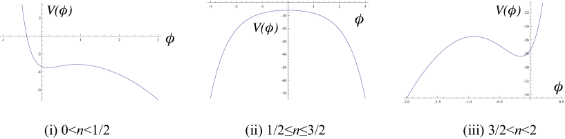
Figure 1: The behaviour of the scalar potential for (i) $0<n<1/2$, (ii) $1/2<n<3/2$ and (iii) $3/2<n<2$. The $1/2\leq n<3/2$ case admits only a global maximum corresponding to the supersymmetric vacuum, otherwise there exist two critical points. The extrema always correspond to a negative cosmological constant.

If we define $\phi\equiv\phi_{1}+\delta\phi$ and expand the potential around $\phi_{1}$, the action (13) can be written as

$$S=\int\left[\frac{R-2\Lambda}{2}-\frac{1}{2}g^{\mu\nu}\partial_{\mu}\delta\phi\,\partial_{\nu}\delta\phi-\frac{1}{2}m^{2}\delta\phi^{2}+{\cal O}(\delta\phi^{3})\right]\sqrt{-g}\,{\rm d}^{4}x\,,$$ (20)

with the cosmological constant $\Lambda=-3\ell^{-2}$, where the asymptotic AdS curvature radius is given by

$$\ell=\frac{\rho_{0}}{2\sqrt{2}g_{0}}\,,\qquad\rho_{0}\equiv\frac{n}{\sqrt{2}}\left(\frac{(2-n)g_{0}}{ng_{1}}\right)^{1-n/2}\,.$$ (21)

The dimensionless parameter $\rho_{0}$ was introduced for later convenience. The mass parameter $m$ measures the curvature of the potential at the supersymmetric critical point and reads

$$m^{2}=-2\ell^{-2}\,.$$ (22)

This is exactly the value for a conformally coupled scalar field in AdS. One can follow the same steps to show that the other vacuum $\phi=\phi_{2}$ also corresponds to the negative cosmological constant $\Lambda=-3\ell_{2}^{2}$ and its mass spectrum is given by

$$m^{2}=\frac{6}{\ell_{2}^{2}}\,,\qquad\ell_{2}=\frac{n(3-2n)}{4g_{0}(1-n)}\left(\frac{g_{0}(2-n)(1-2n)}{g_{1}n(3-2n)}\right)^{1-n/2}\,.$$ (23)

The supersymmetric vacua ($\partial_{\phi}W=0$) are always stable since the mass is above or equal to the Breitenlohner-Freedman (BF) bound Breitenlohner:1982jf , which can be grasped as

$$m^{2}=\partial_{\phi}^{2}V=8\left[2\left(\partial_{\phi}^{2}W-\frac{3}{4}W\right)^{2}-\frac{9}{8}W^{2}\right]\geq-9W^{2}=m_{\rm BF}^{2}\,,$$ (24)

where $m_{\rm BF}^{2}=-9/(4\ell^{2})$ denotes the BF mass bound and the above mass (22) indeed exceeds this lower bound. Here, it is important to remark that the mass (22) at the vacuum $\phi_{1}$ lies in the BF range Breitenlohner:1982jf

$$m^{2}_{\text{BF}}\leq m^{2}\leq m^{2}_{\text{BF}}+\frac{1}{\ell^{2}}\,.$$ (25)

By requiring the conservation and the positivity of a suitable energy functional, Breitenlohner and Freedman Breitenlohner:1982jf found that the slowly decaying mode of the scalar field is also normalizable when the mass parameter lies in this range. It was later shown by Ishibashi and Wald Ishibashi:2004wx that this is also a necessary condition for stability of the scalar field. They proved that the Hamiltonian operator of various fields admits a positive, self-adjoint extension if and only if the mass is above or equal to the BF bound (see proposition 3.1 in ref. Ishibashi:2004wx ). They also showed that the extension of the Hamiltonian is specified by a single parameter taking values in $\mathbb{R}\text{P}^{1}\cong\text{S}^{1}$ when the mass of the scalar field lies in the BF range, and that the possible choices of self-adjoint extension correspond to the freedom of choosing possible boundary conditions specified by that parameter. This parameter appears in the asymptotic behaviour of the scalar field as follows. Let $r$ denote the standard radial coordinate of AdS. Then the free scalar field $\phi$ propagating in AdS behaves at infinity as

$$\phi\sim\frac{\phi_{\pm}(x^{i})}{r^{\lambda_{\pm}}}\,,\qquad\lambda_{\pm}=\frac{1}{2}(3\pm\sqrt{9+4m^{2}\ell^{2}})\,,$$ (26)

where $x^{i}$ are coordinates on the conformal boundary. For the vacuum $\phi=\phi_{1}$, this gives $\lambda_{+}=2$ and $\lambda_{-}=1$. When $m^{2}\geq m^{2}_{\rm BF}+1/\ell^{2}$ as in the vacuum $\phi_{2}$, the allowed boundary condition is only of Dirichlet type, and thus $\phi_{-}(x^{i})=0$. For the BF range (25), $\phi_{-}(x^{i})$ can also be nonvanishing and the ratio corresponding to the mixed boundary condition is characterized by a single dimensionless parameter $\alpha$ as Hertog:2004dr

$$\phi\sim\frac{\phi_{-}(x^{i})}{r^{\lambda_{-}}}+\frac{\alpha\phi_{-}^{\lambda_{+}/\lambda_{-}}(x^{i})}{r^{\lambda_{+}}}\,.$$ (27)

This relation is crucial for determining the mass of the spacetime in a later section.

3 Black holes with scalar hair

In this section, we construct black hole solutions with a nontrivial scalar profile in the Einstein-scalar theory described by the action (13). The equations of motion following from (13) read

$$\Box\phi=V^{\prime}(\phi)\,,\qquad R_{\mu\nu}=\partial_{\mu}\phi\,\partial_{\nu}\phi+g_{\mu\nu}V(\phi)\,,$$ (28)

where the potential is given by (15). As we are looking for static black holes, we use the ansatz

$${\rm d}s^{2}=-\,e^{2X(r)}{\rm d}t^{2}+e^{-2X(r)}{\rm d}r^{2}+e^{2Y(r)}{\rm d}\Sigma_{k}^{2}\,,\qquad\phi=\phi(r)\,,$$ (29)

where ${\rm d}\Sigma_{k}^{2}$ is the line element on a two-dimensional space with constant curvature $k$,

$${\rm d}\Sigma_{k}^{2}=\frac{{\rm d}\chi^{2}}{1-k\chi^{2}}+\chi^{2}{\rm d}\varphi^{2}\,,\qquad k=0,\pm 1\,.$$ (30)

Introducing the new function $\psi=X+Y$, the equations of motion (28) boil down to

$$\begin{split}&X^{\prime\prime}+2X^{\prime}\psi^{\prime}=-e^{-2X}V(\phi)\,,\\ &\psi^{\prime\prime}+2\psi^{\prime 2}-ke^{-2\psi}=-2e^{-2X}V(\phi)\,,\\ &\phi^{\prime\prime}+2\phi^{\prime}\psi^{\prime}=e^{-2X}V^{\prime}(\phi)\,,\\ &X^{\prime 2}-\psi^{\prime 2}+\frac{1}{2}\phi^{\prime 2}+ke^{-2\psi}=e^{-2X}V(\phi)\,.\end{split}$$ (31)

It is worth noting that the equations (31) may also be derived from the one-dimensional action

$$S=\int\left[\frac{1}{2}e^{2\psi}\left(-X^{\prime 2}+\psi^{\prime 2}-\frac{1}{2}\phi^{\prime 2}\right)-\frac{1}{2}e^{-2X+2\psi}V(\phi)\right]{\rm d}r\,.$$ (32)

Since $r$ does not appear explicitely in the Lagrangian, the Hamiltonian $H$ is constant, and from the last equation of (31) we see that $H$ coincides with $k/2$.

Inspired by Klemm:2012yg we set

$$e^{2Y(r)}=f_{1}(r)^{n}f_{2}(r)^{2-n}\,.$$ (33)

Then it turns out that a class of solutions to the equations of motion (31) is given by

$$f_{1}=\frac{n}{\sqrt{2}}\left(r+\frac{2\beta}{n}\right)\,,\qquad f_{2}=\frac{2-n}{\sqrt{2}}\frac{g_{0}}{g_{1}}\left(r-\frac{2\beta}{2-n}\right)\,,$$

$$e^{2\psi}=8g_{0}^{2}\left(r+\frac{2\beta}{n}\right)\left(r-\frac{2\beta}{2-n}\right)\left(r^{2}-\frac{4(1-n)}{n(2-n)}\beta r+4\frac{5n^{2}-10n+4}{n^{2}(2-n)^{2}}\beta^{2}+\frac{k}{8g_{0}^{2}}\right)\,,$$

$$e^{\lambda_{n}\phi}=\frac{g_{0}(2-n)}{g_{1}n}\,\frac{r-2\beta/(2-n)}{r+2\beta/n}\,,$$ (34)

where $\beta$ denotes an arbitrary constant. The metric becomes then

$${\rm d}s^{2}=-\frac{e^{2\psi}}{f_{1}^{n}f_{2}^{2-n}}{\rm d}t^{2}+\frac{f_{1}^{n}f_{2}^{2-n}}{e^{2\psi}}{\rm d}r^{2}+f_{1}^{n}f_{2}^{2-n}{\rm d}\Sigma_{k}^{2}\,.$$ (35)

Note that the solution is given in terms of a quartic polynomial $e^{2\psi}$ and two linear functions $f_{1},f_{2}$, whose powers reflect the expression for the prepotential. This generic structure was first observed in Cacciatori:2009iz . When $\beta=0$, we recover AdS in static coordinates with a two-dimensional constant curvature space ${\rm d}\Sigma_{k}^{2}$. Hence $\beta$ measures the deviation from AdS and is proportional to the mass of the black hole, as we will see later. If we take the limit $g_{0}\to 0$ with $g_{1}/g_{0}$ kept finite, the potential vanishes and the spacetime reduces to the asymptotically flat metric found in Janis:1968zz ; Wyman:1981bd , which describes a naked singularity. It follows that our solution does not include asymptotically flat black holes with scalar hair. It is also worthwhile to remark that the only way to kill the scalar field is $\beta=0$, hence the solution (35) is disconnected from the (topological) Schwarzschild-AdS family. As we will see, the metric (35) admits a parameter range that allows a regular event horizon with a nontrivial scalar field. (35) provides thus a novel example describing a hairy black hole.

3.1 Comparison with other literature

Before going into the details of our solution, it is useful to compare it with other asymptotically AdS hairy black holes previously constructed in the literature. Some of them turn out to correspond actually to a subclass of (3), (35).

The first class is the special case $n=1/2$ and $k=1$ presented in Lu:2013ura , which represents an exact solution of the theory obtained by the single scalar truncation of ${\rm U}(1)^{4}\subset{\rm SO}(8)$ gauged supergravity. Setting $\beta_{2}=0$ and subsequently taking the limit $\beta_{1}\to\infty$ in eq. (2.1) of Lu:2013ura , we obtain the metric

$${\rm d}s^{2}=-(1+g^{2}r^{2})\sqrt{f_{0}}{\rm d}t^{2}+\frac{{\rm d}r^{2}}{(1+g^{2}r^{2})\sqrt{f_{0}}}+r^{2}\sqrt{f_{0}}\,{\rm d}\Omega_{2}^{2}\,,$$ (36)

and the scalar field

$$\phi=-\frac{\sqrt{3}}{2}\log f_{0}\,,$$ (37)

where $f_{0}=1-2\mu/r$. From the expression of the potential we learn that $g^{2}=g_{0}^{2}\rho_{0}^{-2}$ and it is straightforward to check that the metric (36) can be put in the form (35) through the transformations $r\to\rho_{0}\left(r-\frac{4}{3}\beta\right)$, $t\to\rho_{0}^{-1}t$ and requiring that $\mu=-\frac{8}{3}\beta\rho_{0}$.

If one takes instead $n=1/2$, $k=-1$ and $g_{1}=3g_{0}$, (3), (35) boils down to the MTZ black hole Martinez:2004nb .

Another interesting solution with scalar hair was obtained in Anabalon:2012ta ; Feng:2013tza . In these papers a general ansatz for the metric and the scalar field are presented, and the expression of the potential is derived by requiring the equations of motion to hold. Although the produced potential in general fails to have a physical motivation, a subclass of it ($\alpha=0$ in their notation) is inspired by supergravity. Tailoring to the present normalization (13), the four-dimensional solution in Feng:2013tza reads

$${\rm d}s^{2}=-\frac{f(r)}{H_{1}^{1+\mu}(r)H_{2}^{1-\mu}(r)}{\rm d}t^{2}+H_{1}^{1+\mu}(r)H_{2}^{1-\mu}(r)\left(\frac{{\rm d}r^{2}}{f(r)}+r^{2}{\rm d}\Sigma_{k}^{2}\right)\,,$$ (38)

where

$$H_{i}=1+\frac{q_{i}}{r}\,,\qquad f=kH_{1}H_{2}+g^{2}r^{2}(H_{1}^{1+\mu}H_{2}^{1-\mu})^{2}\,,\qquad\phi=\frac{\nu}{\sqrt{2}}\ln\left(\frac{H_{1}}{H_{2}}\right)\,.$$ (39)

Their scalar potential is given by

$$V=-\frac{1}{2}g^{2}e^{\sqrt{2}(\mu-1)\phi/\nu}\left[(\mu-1)(2\mu-1)e^{2\sqrt{2}\phi/\nu}-4(\mu^{2}-1)e^{\sqrt{2}\phi/\nu}+(\mu+1)(2\mu+1)\right]\,.$$ (40)

Here $\mu,\nu$ are constants satisfying $\mu^{2}+\nu^{2}=1$. If we set

$$\mu=\pm(n-1)\,,\qquad\nu=\pm\sqrt{n(2-n)}\,,$$ (41)

we can recover our potential (15) with $g_{0}=gn/4$, $g_{1}=g(2-n)/4$ Lu:2013eoa . The solution (38) does not have an event horizon for $k\geq 0$, but is very similar to ours. In fact, taking e.g. the plus sign in (41), one sees that (38) is of the form (35) with the $f_{i}$ proportional to $rH_{i}$. However, it turns out that the sign of $\phi$ in (39) and (3) disagrees. Moreover, the function $\psi$ that results from casting (38) into the form (35) is different from $\psi$ in (3). It follows that the static solution (38) corresponds to a branch different from ours. It would be very interesting to seek for a solution that comprises both (3), (35) and (38), (39). An ansatz for $\psi$ and $\phi$ that in principle does this job would be

$$e^{2\psi}=f_{1}(r)f_{2}(r)[c_{1}r^{2}+c_{2}r+c_{3}+c_{4}f_{1}(r)^{2n-1}f_{2}(r)^{3-2n}]\,,\qquad\lambda_{n}\phi=\ln\left(c_{0}\frac{f_{2}(r)}{f_{1}(r)}\right)\,,$$ (42)

with $f_{i}(r)=a_{i}r+b_{i}$, where $a_{i},b_{i},c_{i}$ are constants. Indeed, our solution has $c_{4}=0$, while (38) would correspond to $c_{1}=c_{2}=0$. Unfortunately it turns out that (42) works either for (3), (35) or for (38), (39), but is unable to synthesize both. We shall leave the construction of such a more general solution for future work.

Let us finally compare with the spherically symmetric numerical solution discussed in Hertog:2004bb . Our Lagrangian reduces to theirs when $n=1$ with $g_{0}=g_{1}$. Hence one may hope that our solution represents their numerical solution. However, our metric does not admit a spherical horizon when $n=1$, as we will see in the next section. This fact also suggests to look for more general solutions that contain both (3), (35) and the numerical one of Hertog:2004bb .

4 Physical discussion

In this section, we explore various properties of the hairy black hole obtained in the previous section.

4.1 Mass

The mass of a given spacetime is the most fundamental physical quantity. Let us therefore try to identify a well-defined mass for our spacetime. Since the conserved charges defined at infinity are usually encoded in the leading terms of physical fields departing from the background spacetime, we consider the asymptotic behavior of the metric and the scalar field. For this purpose, it is convenient to define the areal radius by

$$\rho=\sqrt{f_{1}^{n}f_{2}^{2-n}}\,.$$ (43)

In terms of $\rho$, the asymptotic expansion ($\rho\to\infty$) of the metric (35) reads

$${\rm d}s^{2}\simeq-\left(k+\frac{\rho^{2}}{\ell^{2}}-\frac{2\mu_{1}}{\rho}\right){\rm d}\tau^{2}+\left(k+\gamma+\frac{\rho^{2}}{\ell^{2}}-\frac{2\mu_{2}}{\rho}\right)^{-1}{\rm d}\rho^{2}+\rho^{2}{\rm d}\Sigma_{k}^{2}\,,$$ (44)

where $\tau=\rho_{0}^{-1}t$, $\ell=\rho_{0}/(2\sqrt{2}g_{0})$ is the AdS radius given in (21) and

$$\gamma\equiv\frac{32g_{0}^{2}\beta^{2}}{n(2-n)}\,.$$ (45)

We have also defined the two parameters

$$\mu_{1} =\frac{1}{12}\rho_{0}\lambda_{n}^{6}(n-1)\beta[3kn^{2}(n-2)^{2}+128g_{0}^{2}\beta^{2}(3-2n)(1-2n)]\,,$$ (46a)

$$\mu_{2} =\frac{1}{12}\rho_{0}\lambda_{n}^{6}(n-1)\beta[3kn^{2}(n-2)^{2}+128g_{0}^{2}\beta^{2}(5n^{2}-10n+3)]\,.$$ (46b)

The scalar field behaves according to (26),

$$\phi\simeq\phi_{1}+\frac{\phi_{-}}{\rho}+\frac{\phi_{+}}{\rho^{2}}+{\cal O}(1/\rho^{3})\,,$$ (47)

where $\phi_{1}$ is defined by (19) and

$$\phi_{-}=-2\lambda_{n}\beta\rho_{0}\,,\qquad\phi_{+}=-2(n-1)\lambda_{n}^{3}\beta^{2}\rho_{0}^{2}\,.$$ (48)

It follows that the parameter $\alpha$ in (27) characterizing the boundary condition reads

$$\alpha=\frac{1}{2}(1-n)\lambda_{n}\,.$$ (49)

We also note the useful relation

$$\gamma=\frac{1}{2\ell^{2}}\phi_{-}^{2}\,.$$ (50)

Thus far, various notions of asymptotically AdS spacetimes have been defined Abbott:1981ff ; Ashtekar:1984zz ; Henneaux:1985tv ; Hollands:2005wt , and lots of apparently distinct definitions of conserved charges have been proposed. Unfortunately, asymptotic AdS boundary conditions put forward in these papers do not allow a class of metrics behaving like (44). Due to the fact that the mass of the scalar field lies in the range (25), the stress tensor of the slowly decaying mode $\phi_{-}$ of the scalar field does not fall off sufficiently rapidly at infinity, giving rise to a backreaction to the geometry which modifies the $g^{\rho\rho}$ behaviour from the standard asymptotic form with $\gamma=0$. This is a main obstruction to construct the conserved quantity following the prescriptions in Abbott:1981ff ; Ashtekar:1984zz ; Henneaux:1985tv ; Hollands:2005wt . This property is also encoded into the behavior of the Misner-Sharp energy Misner:1964je , which is a well-defined quasi-local energy in pseudo-spherical symmetry Maeda:2007uu and is defined by

$$M_{\rm MS}=\frac{1}{2}\rho\left[k-(\nabla\rho)^{2}+\frac{\rho^{2}}{\ell^{2}}\right]\,.$$ (51)

One easily sees that it diverges as $\rho\to\infty$ for our spacetime (35).

Hertog and Maeda proposed a possible way to avoid this problem Hertog:2004dr . They generalized the boundary conditions of Henneaux-Teitelboim Henneaux:1985tv in such a way that the relaxed boundary conditions (i) include spacetimes containing a scalar field with mass parameter in the BF range, (ii) are invariant under the asymptotic symmetries (eq. (2.14) of Hertog:2004dr ), and (iii) allow charges generated by the corresponding asymptotic symmetries to remain finite. Focusing on the asymptotically globally AdS case ($k=1$), they obtained Hertog:2004dr

$$Q[\xi]=Q_{\rm HT}[\xi]+\frac{\lambda_{-}}{16\pi\ell}\oint{\rm d}\Omega_{2}{\xi^{\bot}}r^{2}\left(\phi^{2}+\frac{2}{3}\alpha(\lambda_{+}-\lambda_{-})\phi^{3/\lambda_{-}}\right)\,,$$ (52)

where $\xi$ is an asymptotic symmetry and $\xi^{\bot}$ denotes its normal component to the spacelike surface. $Q_{\rm HT}[\xi]$ denotes the contribution of the Henneaux-Teitelboim charge Henneaux:1985tv . We would like to stress that this piece is divergent, which is precisely cancelled by the divergence of the second term. In the present case, the mass is given by $M=Q[\rho_{0}\partial_{t}]$, i.e.,

$$M=\mu_{2}-\frac{32}{3}g_{0}^{2}\rho_{0}n(2-n)(1-n)\lambda_{n}^{6}\beta^{3}=\mu_{1}\,,$$ (53)

where the last equality was evaluated by using (46a). The constant of integration has been fixed so that it vanishes for AdS spacetime. This expression also coincides with the formula given in Henneaux:2006hk ,

$$M=\mu_{2}-\frac{1}{3}m^{2}\alpha\phi_{-}^{3/\lambda_{-}}\,,$$ (54)

where $m$ is the mass (22) at the AdS vacuum $\phi=\phi_{1}$. A natural generalization to the topological cases ($k=0,-1$) is inferred to be

$$M=\frac{\Sigma_{k}\mu_{1}}{4\pi}\,,$$ (55)

where $\Sigma_{k}$ is the area of a unit maximally symmetric space with curvature $k$. We will justify this expression below by deriving the first law of black hole thermodynamics.

The $n=1$ case is particularly interesting since the mass vanishes, whereas the scalar field profile remains nontrivial. This does not contradict the positive mass theorem, since the $n=1$ spherical solution describes a naked singularity as shown in section 4.2.

Note that the parameter $\mu_{1}$ indeed corresponds to the Coulomb part of the spacetime. Namely the Weyl scalar of the Newman-Penrose formalism behaves as

$$\Psi_{2}=-\frac{\mu_{1}}{\rho^{3}}+{\cal O}(1/\rho^{4})\,.$$ (56)

This behaviour partly justifies the use of the Ashtekhar-Magnon definition of conserved charges Ashtekar:1984zz for spacetimes with scalar field in the BF range, since their mass essentially corresponds to the coefficient of the ${\cal O}(1/\rho^{3})$ term of the electric part of the Weyl tensor. Considering the fall-off behaviour of the stress-energy tensor in Ashtekar:1984zz , there does not appear to be an a priori reason why the Ashtekhar-Magnon charge is finite in the present case. Perhaps it appears that some miraculous cancellation occurs between terms arising from the metric and the scalar field.

4.2 Horizon structure

There appear two possible Killing horizons $r_{\pm}$, which are identified by the two roots of $e^{2\psi}=0$, i.e.,

$$r_{\pm}=\frac{8g_{0}\beta(1-n)\pm\sqrt{-2kn^{2}(2-n)^{2}-64g_{0}^{2}\beta^{2}(3-8n+4n^{2})}}{4g_{0}n(2-n)}\,.$$ (57)

$r=r_{+}$ describes the event horizon of a black hole, on which we focus hereafter. The other roots $r=-2\beta/n$ and $r=2\beta/(2-n)$ are not our concern, since they correspond to a curvature singularity. This can be easily seen by noting that the areal radius $\rho$ defined by (43) vanishes at these points.

Let us first discuss the conditions under which spherical horizons exist. Setting $k=1$ in (57), the expression under the square root is nonnegative for $1/2<n<3/2$ and

$$32g_{0}^{2}\beta^{2}\geq-\frac{n^{2}(2-n)^{2}}{3-8n+4n^{2}}\,.$$ (58)

In addition, we must impose that the curvature singularities at $r=-2\beta/n$ and $r=2\beta/(2-n)$ be hidden behind the horizon. It turns out that this yields a lower bound on $g_{0}^{2}\beta^{2}$ that is more stringent than (58). A straightforward calculation shows that spherical black holes exist for

$$\frac{1}{2}<n<1\quad\text{and}\quad g_{0}\beta>\frac{n(2-n)}{8\sqrt{2}\sqrt{(2n-1)(1-n)}}$$ (59)

or

$$1<n<\frac{3}{2}\quad\text{and}\quad g_{0}\beta<-\frac{n(2-n)}{8\sqrt{2}\sqrt{(3-2n)(n-1)}}\,.$$ (60)

Note that for $n=1$ and $k=1$ the solution describes a naked singularity, since in this case either the dangerous radius $2\beta$ (for $\beta>0$) or $-2\beta$ (for $\beta<0$) is larger than $r_{+}$. In the $k=1$ case, the inner horizon $r=r_{-}$ is always smaller than ${\rm max}[-2\beta/n,2\beta/(2-n)]$. This means that the singularity is spacelike and the causal structure is the same as for the $k=1$ Schwarzschild-AdS black hole.

An analogous computation shows that flat horizons ($k=0$) are possible for $1/2<n<1$ and $\beta>0$ or for $1<n<3/2$ and $\beta<0$. In the special case $n=1$ the horizon always coincides with one of the singularities. For the planar case, the inner horizon $r_{-}$ cannot be larger than the singularity at ${\rm max}[-2\beta/n,2\beta/(2-n)]$.

Finally, hyperbolic black holes ($k=-1$) exist if $\beta$ satisfies the following conditions:

• $0<n<1/2$:

  $$-\frac{n(2-n)}{8\sqrt{2}\sqrt{(n-1)(2n-3)}}<g_{0}\beta\leq\frac{n(2-n)}{4\sqrt{2}\sqrt{(2n-1)(2n-3)}}\,,$$ (61)

• $1/2\leq n<1$:

  $$g_{0}\beta>-\frac{n(2-n)}{8\sqrt{2}\sqrt{(n-1)(2n-3)}}\,,$$ (62)

• $1<n\leq 3/2$:

  $$g_{0}\beta<\frac{n(2-n)}{8\sqrt{2}\sqrt{(n-1)(2n-1)}}\,,$$ (63)

• $3/2<n<2$:

  $$-\frac{n(2-n)}{4\sqrt{2}\sqrt{(2n-1)(2n-3)}}\leq g_{0}\beta<\frac{n(2-n)}{8\sqrt{2}\sqrt{(n-1)(2n-1)}}\,.$$ (64)

For $n=1$ there is no restriction on $\beta$. When (61) or (64) are satisfied the inner horizon $r_{-}$ also appears, since it is larger than ${\rm max}[-2\beta/n,2\beta/(2-n)]$.

In the case $k=-1$, $r_{+}$ and $r_{-}$ can actually coincide. One finds that extremal hyperbolic hairy black holes exist when

$$0<n<\frac{1}{2}\quad\text{and}\quad g_{0}\beta=\frac{n(2-n)}{4\sqrt{2}\sqrt{(3-2n)(1-2n)}}$$ (65)

or

$$\frac{3}{2}<n<2\quad\text{and}\quad g_{0}\beta=-\frac{n(2-n)}{4\sqrt{2}\sqrt{(3-2n)(1-2n)}}\,.$$ (66)

The extremal solution interpolates between AdS₄ at infinity and $\text{AdS}_{2}\times\text{H}^{2}$ at the horizon. Interestingly, the value of the scalar field at the horizon agrees with the other critical point of the potential at $\phi=\phi_{2}$. It follows that the scalar field goes thereby from the supersymmetric vacuum $\phi_{1}$ at $r=\infty$ to $\phi=\phi_{2}$ at the horizon. We explicitly checked that the near-horizon geometry with $\phi=\phi_{2}$ breaks supersymmetry. From the holographic point of view, the black hole describes a ($2+1$)-dimensional superconformal field theory that is perturbed by a multi-trace deformation and flows to a conformal quantum mechanics in the IR (‘flow across dimensions’) Witten:2001ua ; Papadimitriou:2007sj .

4.3 Thermodynamics

Let us next discuss thermodynamic properties of the black holes. In terms of the horizon radius $r_{+}$, the area of the black hole horizon reads

$$A=\Sigma_{k}f_{1}^{n}(r_{+})f_{2}^{2-n}(r_{+})\,.$$ (67)

From (44), the unit time translation at AdS infinity corresponds to $\xi=\rho_{0}\partial/\partial t$, which is timelike outside and null on the event horizon. The surface gravity, $\kappa^{2}=-\frac{1}{2}\nabla_{\mu}\xi_{\nu}\nabla^{\mu}\xi^{\nu}$, is then easily computed to give

$$\kappa=\left.\frac{(e^{2\psi})^{\prime}}{2\sqrt{2}g_{0}^{(-2+n)/2}g_{1}^{(2-n)/2}n^{-n/2}(2-n)^{(n-2)/2}f_{1}^{n}f_{2}^{2-n}}\right|_{r=r_{+}}\,,$$ (68)

which accords with the Euclidean prescription of removing conical singularities. The Hawking temperature is then defined by $T=\kappa/2\pi$. An elementary computation reveals that the first law of black hole thermodynamics Bardeen:1973gs holds,

$$\delta M=\frac{\kappa}{8\pi}\delta A\,.$$ (69)

It turns out that the scalar charge fails to contribute to the 1st law, consistent with the analysis in Papadimitriou:2005ii . Due to the appearance of a curvature scale, there is no straightforward expression for an integrated mass formula.

Fig. 2 shows the temperature and the horizon area as functions of the mass for $k=1$ and $n=3/4$ (in red), as compared to the Schwarzschild-AdS solution (blue). One can see that the qualitative behaviour is very similar to that of the Schwarzschild-AdS black hole. There appears a critical temperature $T_{\text{c}}$ above which we have two kinds of black holes with $M\lessgtr M_{\text{c}}$ Hawking:1982dh . We do not write down the explicit expression for $T_{\text{c}}$ since it is quite messy, but it can be easily computed. The behaviour of the specific heat $C=T\partial S/\partial T$ is also similar to the Schwarzschild-AdS black hole, since one has $C\lessgtr 0$ for $M\lessgtr M_{\text{c}}$ and $C\to\pm\infty$ for $M\to M_{\text{c}}\pm 0$.

One sees from fig. 2 that, for a given mass, the area of the hairy black hole is always smaller than the one of the Schwarzschild-AdS black hole, which implies that the hairy black hole is unstable. Such an instability was actually also found for the numerical solutions in the literature Torii:2001pg ; Hertog:2004bb . We shall verify in section 4.4 that our solution admits also an unstable mode.

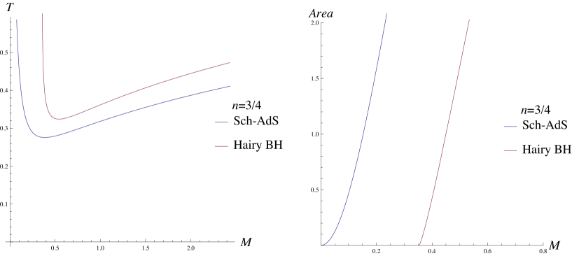
Figure 2: The behaviour of temperature and area as functions of the mass for $k=1$, $n=3/4$. The asymptotic AdS radius has been set to $\ell=1$ and the corresponding quantities for the Schwarzschild-AdS black hole are also shown. Both black holes have a critical temperature. Our black hole solution has a positive mass bound and a smaller entropy compared to the Schwarzschild-AdS black hole.

In the case of a hyperbolic horizon ($k=-1$), there appears an inner horizon outside the curvature singularities. The area product of the two Killing horizons is given by

$$A_{+}A_{-}= \frac{\Sigma_{k}^{2}}{256g_{0}^{4}n^{4}}\left(\frac{n}{2-n}\right)^{2n}\left[kn^{2}(2-n)^{2}+128g_{0}^{2}(1-n)(3-2n)\beta^{2}\right]^{n}$$

$$\times\left[kn^{2}(2-n)^{2}+128g_{0}^{2}(1-n)(1-2n)\beta^{2}\right]^{2-n}\,.$$ (70)

According to the analysis in Cvetic:2010mn , the area product of a generic black hole depends only on the (quantized) charges, the angular momenta and the cosmological constant. However, the right hand side of (4.3) does not correspond to such a quantity. It would be interesting to explore the physical meaning of the right hand side of (4.3).

4.4 Instability against radial perturbations

The behaviour of the entropy of our hairy black hole with respect to Schwarzschild-AdS (fig. 2) implies that our solution is unstable against dynamical perturbations. Focusing on spherically symmetric perturbations, we show that this is indeed the case.

The background spacetime we consider is the spherical solution ($k=1$) of the form

$$g_{\mu\nu}^{(0)}{\rm d}x^{\mu}{\rm d}x^{\nu}=-f(r){\rm d}t^{2}+\frac{{\rm d}r^{2}}{f(r)}+\rho(r)^{2}({\rm d}\theta^{2}+\sin^{2}\theta{\rm d}\varphi^{2})\,,\qquad\phi^{(0)}=\phi^{(0)}(r)\,,$$ (71)

where $f=e^{2\psi}/(f_{1}^{n}f_{2}^{2-n})$ and $\rho(r)$ is given by (43). Here and in what follows, we attach $(0)$ to denote the background quantities. The governing equations are

$$E^{\mu}{}_{\nu}\equiv R^{\mu}{}_{\nu}-\frac{1}{2}R\delta^{\mu}{}_{\nu}-T^{\mu}{}_{\nu}=0\,,\qquad E_{\phi}\equiv\nabla^{\mu}\nabla_{\mu}\phi-\partial_{\phi}V=0\,.$$ (72)

Let us consider the spherically symmetric perturbations

$$g_{\mu\nu}\simeq g^{(0)}_{\mu\nu}+g^{(1)}_{\mu\nu}(r)e^{-i\omega t}\,,\qquad\phi\simeq\phi^{(0)}+\phi^{(1)}(r)e^{-i\omega t}\,,$$ (73)

where $(1)$ corresponds to the perturbed value. Using the gauge freedom $g^{(1)}_{\mu\nu}\to g^{(1)}_{\mu\nu}+\mbox{$\mathscr{L}$}_{\xi}g_{\mu\nu}^{(0)}$, we can work in a gauge where only $g^{(1)}_{tt}$ and $g^{(1)}_{rr}$ are nonvanishing (see Ishibashi:2011ws for a review of gravitational perturbations in spherically symmetric spacetimes).

Using the background Einstein’s equations $E^{(0)}_{\mu\nu}=0$ and linearized Einstein’s equations $E^{(1)}_{\mu\nu}=0$, the perturbed scalar equation $E^{(1)}_{\phi}=0$ reduces to the single master equation

$$\left(-\frac{{\rm d}^{2}}{{\rm d}r_{*}^{2}}+U(r)\right)\Phi=\omega^{2}\Phi\,,$$ (74)

where $\Phi=\rho\phi^{(1)}$ and $r_{*}=\int{\rm d}r/f(r)$ denotes the tortoise coordinate. The potential $U(r)$ reads

$$U=\frac{f}{2\rho\rho^{\prime}{}^{2}}[f\rho^{3}(\phi^{(0)})^{\prime}{}^{4}+2\rho^{\prime 2}(f\rho^{\prime})^{\prime}-2\rho\rho^{\prime}(f\rho)^{\prime}(\phi^{(0)})^{\prime}{}^{2}+4\rho^{2}\rho^{\prime}(\phi^{(0)})^{\prime}V_{\phi}+2\rho\rho^{\prime}{}^{2}V_{\phi\phi}]\,,$$ (75)

where the prime denotes the differentiation with respect to $r$, $V_{\phi}=\partial_{\phi}V$ and $V_{\phi\phi}=\partial_{\phi}^{2}V$ correspond to the background value. The tortoise coordinate asymptotically behaves as

$$r_{*}\sim\frac{1}{f^{\prime}(r_{+})}\ln(r-r_{+})\to-\infty\leavevmode\nobreak\ \leavevmode\nobreak\ (r\to r_{+})\,,\qquad r_{*}\sim-\frac{\ell^{2}}{r}+K\leavevmode\nobreak\ \leavevmode\nobreak\ (r\to\infty)\,,$$ (76)

where $K$ is a constant.

We are now looking for an unstable mode which occurs at a purely imaginary frequency. Hence we set $\sigma=-i\omega$ ($\sigma>0$) as in ref. Hertog:2004bb . Since $U\to 0$ for $r_{*}\to-\infty$, the normalizable asymptotic solution at the horizon reads

$$\Phi\sim\exp(\sigma r_{*})\,,\qquad(r_{*}\to-\infty)\,.$$ (77)

Let us next consider the boundary condition for $\Phi$ at infinity. The scalar field behaves as

$$\phi\sim\frac{\phi_{-}}{\rho}+\frac{\alpha\phi_{-}^{2}}{\rho^{2}}\,.$$ (78)

Hence for $\phi=\phi^{(0)}+\phi^{(1)}e^{-i\omega t}$ we have

$$\phi^{(1)}\sim\frac{\phi_{-}^{(1)}}{\rho}+\frac{2\alpha\phi_{-}^{(0)}\phi_{-}^{(1)}}{\rho^{2}}\,.$$ (79)

Let $U_{0}=U(r\to\infty)<0$ and suppose $\tilde{\sigma}=\sqrt{-U_{0}-\sigma^{2}}$ is positive. Then the asymptotic solution reads

$$\Phi\sim A\cos(\tilde{\sigma}r_{*}+b)\simeq A\left[\cos(\tilde{\sigma}K+b)+\frac{\tilde{\sigma}\ell^{2}}{r}\sin(\tilde{\sigma}K+b)\right]\,,$$ (80)

where $A$ and $b$ are constants. Noting $\rho\sim\rho_{0}(r+\mbox{$\mathcal{O}$}(1/r))$, a comparison of (79) and (80) gives

$$\tilde{\sigma}\ell^{2}\tan(\tilde{\sigma}K+b)=\frac{2\alpha\phi_{-}^{(0)}}{\rho_{0}}\,.$$ (81)

This translates into

$$\frac{{\rm d}}{{\rm d}r_{*}}\Phi\simeq-\frac{2\alpha\phi_{-}^{(0)}}{\rho_{0}\ell^{2}}\Phi\quad(r\to\infty)\,.$$ (82)

We now have a Schrödinger-type equation (74) with the boundary conditions (77), (82). We numerically solved the eigenvalue problem and found an unstable mode as displayed in fig. 3. As $\beta$ increases, the instability rate becomes smaller. Since we fix the AdS curvature, large $\beta$ means large horizon radius. Thus the smaller hairy black hole is more unstable. For the chosen values $n=3/4$, $g_{0}=\ell=1$, the unstable mode seems to disappear around $\beta\sim 1.4$. The profound physical reason for this value and its relation to thermodynamics remain still to be understood.

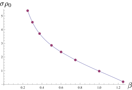
Figure 3: Instability rate against radial perturbations for $n=3/4$, $g_{0}=\ell=1$.

4.5 Asymptotically de Sitter case

A Wick rotation of the coupling constants, $g_{0}\to ig_{0}$, $g_{1}\to ig_{0}$, reverses the sign of the scalar potential, hence the metric is asymptotically de Sitter. The potential is no longer expressed in terms of a real superpotential, yet the solution still solves the equations of motion (28). In eqs. (3), the expressions of $f_{1}$, $f_{2}$ and $\phi$ are left invariant, whereas

$$e^{2\psi}= \left(r+\frac{2\beta}{n}\right)\left(r-\frac{2\beta}{2-n}\right)$$

$$\times\left[k-8g_{0}^{2}\left(r^{2}-\frac{4(1-n)}{n(2-n)}\beta r+4\frac{5n^{2}-10n+4}{n^{2}(2-n)^{2}}\beta^{2}\right)\right]\,.$$ (83)

Our solution is compatible with the no-hair theorem for asymptotically de Sitter spacetimes Bhattacharya:2007zzb since the potential is not convex.

The Killing horizons are given by

$$r_{\text{c}}= \frac{8g_{0}\beta(1-n)+\sqrt{2kn^{2}(2-n)^{2}-64g_{0}^{2}\beta^{2}(3-8n+4n^{2})}}{4g_{0}n(2-n)}\,,$$ (84a)

$$r_{+}= \frac{8g_{0}\beta(1-n)-\sqrt{2kn^{2}(2-n)^{2}-64g_{0}^{2}\beta^{2}(3-8n+4n^{2})}}{4g_{0}n(2-n)}\,.$$ (84b)

$r=r_{\text{c}}$ is a cosmological horizon, while $r=r_{+}\leq r_{\text{c}}$ is a black hole event horizon. It turns out that the condition for the existence of these real roots is weaker than the no naked singularity condition $r_{+}\geq{\rm max}[2\beta/(2-n),-2\beta/n]$. One finds that horizons exist only for $k=1$ with the following parameter region:

• $0<n\leq 1/2$:

  $$\frac{n(2-n)}{8\sqrt{2(1-n)(1-2n)}}<g_{0}\beta\leq\frac{n(2-n)}{4\sqrt{2(1-2n)(3-2n)}}\,,$$ (85)

• $3/2\leq n<2$:

  $$-\frac{n(2-n)}{4\sqrt{2(2n-3)(2n-1)}}\leq g_{0}\beta<-\frac{n(2-n)}{8\sqrt{2(n-1)(2n-3)}}\,.$$ (86)

For these parameter ranges, the global structure is the same as for the $k=1$ Schwarzschild-de Sitter black hole. One can also verify that there exist no lukewarm black holes for which the temperatures of the black hole horizon and the cosmological horizon are equal.

5 Final remarks

In this paper we constructed a new family of black holes with scalar hair in $N=2$ Fayet-Iliopoulos gauged supergravity. A distinguished feature of our solution is that it is sourced only with a scalar field. This kind of exact black hole solution is of importance and will be a stepping stone for constraining the conditions under which the no-hair theorem is valid.

We explored various properties of these black holes. In particular, we pointed out that the standard methods of computing conserved charges does not work, since the asymptotic behaviour of the metric is out of the framework of ‘asymptotically AdS’ proposed in the literature. Nevertheless, we identified a well-defined mass function following the prescription of Hertog and Maeda Hertog:2004dr . This fixes some confusions prevailing in the literature.

One may be tempted to hope that this solution would be a novel counterexample to the no hair conjecture. Since our black hole is unstable, this is not the case. However, this instability is interesting from the holographic viewpoint Gubser:2000mm . It would be nice to see if our solution has some potential applications in the AdS/CFT correspondence, and in particular to condensed matter physics, where one typically includes the leading scalar operator in the dynamics. This is generically uncharged, and is dual to a neutral scalar field in the bulk.

Another possible extension of the present work is to look for rotating black holes. In this case, there might exist a rotating black hole which admits only a helical Killing vector Herdeiro:2014goa . It would be interesting to construct this kind of exact solutions in the framework of supergravity.

References

- (1) W. Israel, “Event horizons in static vacuum space-times,” Phys. Rev. 164 (1967) 1776.
- (2) W. Israel, “Event horizons in static electrovac space-times,” Commun. Math. Phys. 8 (1968) 245.
- (3) B. Carter, “Axisymmetric black hole has only two degrees of freedom,” Phys. Rev. Lett. 26 (1971) 331.
- (4) D. C. Robinson, “Uniqueness of the Kerr black hole,” Phys. Rev. Lett. 34 (1975) 905.
- (5) P. O. Mazur, “Proof of uniqueness of the Kerr-Newman black hole solution,” J. Phys. A 15 (1982) 3173.
- (6) R. H. Price, “Nonspherical perturbations of relativistic gravitational collapse. 1. Scalar and gravitational perturbations,” Phys. Rev. D 5 (1972) 2419.
- (7) R. Ruffini and J. A. Wheeler, “Introducing the black hole,” Phys. Today 24 (1971) 1, 30.
- (8) J. D. Bekenstein, “Nonexistence of baryon number for static black holes,” Phys. Rev. D 5 (1972) 1239.
- (9) J. D. Bekenstein, “Transcendence of the law of baryon-number conservation in black hole physics,” Phys. Rev. Lett. 28 (1972) 452.
- (10) M. Heusler, “A no hair theorem for selfgravitating nonlinear sigma models,” J. Math. Phys. 33 (1992) 3497.
- (11) D. Sudarsky, “A simple proof of a no hair theorem in Einstein Higgs theory,,” Class. Quant. Grav. 12 (1995) 579.
- (12) A. A. H. Graham and R. Jha, “Nonexistence of black holes with noncanonical scalar fields,” Phys. Rev. D 89 (2014) 8, 084056 [arXiv:1401.8203 [gr-qc]].
- (13) J. D. Bekenstein, “Exact solutions of Einstein conformal scalar equations,” Annals Phys. 82 (1974) 535.
- (14) J. D. Bekenstein, “Black holes with scalar charge,” Annals Phys. 91 (1975) 75.
- (15) P. Bizon, “Colored black holes,” Phys. Rev. Lett. 64 (1990) 2844.
- (16) K. A. Bronnikov and Y. N. Kireev, “Instability of black holes with scalar charge,” Phys. Lett. A 67 (1978) 95.
- (17) P. Bizon and R. M. Wald, “The N=1 colored black hole is unstable,” Phys. Lett. B 267 (1991) 173.
- (18) M. Huebscher, P. Meessen, T. Ortín and S. Vaulà, “Supersymmetric Einstein-Yang-Mills monopoles and covariant attractors,” Phys. Rev. D 78 (2008) 065031 [arXiv:0712.1530 [hep-th]].
- (19) M. Huebscher, P. Meessen, T. Ortín and S. Vaulà, “ Einstein-Yang-Mills’ BPS solutions,” JHEP 0809 (2008) 099 [arXiv:0806.1477 [hep-th]].
- (20) P. Meessen, “Supersymmetric coloured/hairy black holes,” Phys. Lett. B 665 (2008) 388 [arXiv:0803.0684 [hep-th]].
- (21) P. Bueno, P. Meessen, T. Ortín and P. F. Ramírez, “ Einstein-Yang-Mills’ static two-center solutions,” JHEP 1412 (2014) 093 [arXiv:1410.4160 [hep-th]].
- (22) P. Meessen and T. Ortín, “ super-EYM coloured black holes from defective Lax matrices,” JHEP 1504 (2015) 100 [arXiv:1501.02078 [hep-th]].
- (23) S. Aretakis, “Stability and instability of extreme Reissner-Nordström black hole spacetimes for linear scalar perturbations I,” Commun. Math. Phys. 307 (2011) 17 [arXiv:1110.2007 [gr-qc]].
- (24) J. Lucietti and H. S. Reall, “Gravitational instability of an extreme Kerr black hole,” Phys. Rev. D 86 (2012) 104030 [arXiv:1208.1437 [gr-qc]].
- (25) P. Bueno and C. S. Shahbazi, “The violation of the no-hair conjecture in four-dimensional ungauged supergravity,” Class. Quant. Grav. 31 (2014) 145005 [arXiv:1310.6379 [hep-th]].
- (26) D. Sudarsky and J. A. Gonzalez, “On black hole scalar hair in asymptotically anti-de Sitter space-times,” Phys. Rev. D 67 (2003) 024038 [gr-qc/0207069].
- (27) M. T. Anderson, P. T. Chrusciel and E. Delay, “Nontrivial, static, geodesically complete vacuum space-times with a negative cosmological constant,” JHEP 0210 (2002) 063 [gr-qc/0211006].
- (28) A. Anabalón, F. Canfora, A. Giacomini and J. Oliva, “Black holes with primary hair in gauged supergravity,” JHEP 1206 (2012) 010 [arXiv:1203.6627 [hep-th]].
- (29) A. Anabalón, “Exact black holes and universality in the backreaction of non-linear sigma models with a potential in (A)dS4,” JHEP 1206 (2012) 127 [arXiv:1204.2720 [hep-th]].
- (30) A. Anabalón, D. Astefanesei and R. Mann, “Exact asymptotically flat charged hairy black holes with a dilaton potential,” JHEP 1310 (2013) 184 [arXiv:1308.1693 [hep-th]].
- (31) P. A. González, E. Papantonopoulos, J. Saavedra and Y. Vásquez, “Four-dimensional asymptotically AdS black holes with scalar hair,” JHEP 1312 (2013) 021 [arXiv:1309.2161 [gr-qc]].
- (32) P. A. González, E. Papantonopoulos, J. Saavedra and Y. Vásquez, “Extremal hairy black holes,” JHEP 1411 (2014) 011 [arXiv:1408.7009 [gr-qc]].
- (33) M. Cadoni and E. Franzin, “Asymptotically flat black holes sourced by a massless scalar field,” arXiv:1503.04734 [gr-qc].
- (34) S. S. Gubser and I. Mitra, “The evolution of unstable black holes in anti-de Sitter space,” JHEP 0108 (2001) 018 [hep-th/0011127].
- (35) P. Breitenlohner and D. Z. Freedman, “Stability in gauged extended supergravity,” Annals Phys. 144 (1982) 249.
- (36) L. F. Abbott and S. Deser, “Stability of gravity with a cosmological constant,” Nucl. Phys. B 195 (1982) 76.
- (37) A. Ashtekar and A. Magnon, “Asymptotically anti-de Sitter space-times,” Class. Quant. Grav. 1 (1984) L39.
- (38) M. Henneaux and C. Teitelboim, “Asymptotically anti-de Sitter spaces,” Commun. Math. Phys. 98 (1985) 391.
- (39) S. Hollands, A. Ishibashi and D. Marolf, “Comparison between various notions of conserved charges in asymptotically AdS-spacetimes,” Class. Quant. Grav. 22 (2005) 2881 [hep-th/0503045].
- (40) J. Katz, J. Bicak and D. Lynden-Bell, “Relativistic conservation laws and integral constraints for large cosmological perturbations,” Phys. Rev. D 55 (1997) 5957 [gr-qc/0504041].
- (41) T. Hertog and K. Maeda, “Black holes with scalar hair and asymptotics in supergravity,” JHEP 0407 (2004) 051 [hep-th/0404261].
- (42) L. Andrianopoli, M. Bertolini, A. Ceresole, R. D’Auria, S. Ferrara, P. Fré and T. Magri, “ supergravity and super Yang-Mills theory on general scalar manifolds: Symplectic covariance, gaugings and the momentum map,” J. Geom. Phys. 23 (1997) 111 [hep-th/9605032].
- (43) A. Van Proeyen, “ supergravity in and its matter couplings,” extended version of lectures given during the semester “Supergravity, superstrings and M-theory” at Institut Henri Poincaré, Paris, november 2000; http://itf.fys.kuleuven.ac.be/toine/home.htm#B
- (44) M. Cvetič, M. J. Duff, P. Hoxha, J. T. Liu, H. Lü, J. X. Lu, R. Martinez-Acosta, C. N. Pope, H. Sati and T. A. Tran, “Embedding AdS black holes in ten dimensions and eleven dimensions,” Nucl. Phys. B 558 (1999) 96 [hep-th/9903214].
- (45) A. Ishibashi and R. M. Wald, “Dynamics in nonglobally hyperbolic static space-times. 3. Anti-de Sitter space-time,” Class. Quant. Grav. 21 (2004) 2981 [hep-th/0402184].
- (46) M. Henneaux, C. Martínez, R. Troncoso and J. Zanelli, “Asymptotically anti-de Sitter spacetimes and scalar fields with a logarithmic branch,” Phys. Rev. D 70 (2004) 044034 [hep-th/0404236].
- (47) A. J. Amsel and M. M. Roberts, “Stability in Einstein-scalar gravity with a logarithmic branch,” Phys. Rev. D 85 (2012) 106011 [arXiv:1112.3964 [hep-th]].
- (48) D. Klemm and O. Vaughan, “Nonextremal black holes in gauged supergravity and the real formulation of special geometry,” JHEP 1301 (2013) 053 [arXiv:1207.2679 [hep-th]].
- (49) S. L. Cacciatori and D. Klemm, “Supersymmetric AdS4 black holes and attractors,” JHEP 1001 (2010) 085 [arXiv:0911.4926 [hep-th]].
- (50) A. I. Janis, E. T. Newman and J. Winicour, “Reality of the Schwarzschild singularity,” Phys. Rev. Lett. 20 (1968) 878.
- (51) M. Wyman, “Static spherically symmetric scalar fields in general relativity,” Phys. Rev. D 24 (1981) 839.
- (52) H. Lü, Y. Pang and C. N. Pope, “AdS dyonic black hole and its thermodynamics,” JHEP 1311 (2013) 033 [arXiv:1307.6243 [hep-th]].
- (53) C. Martínez, R. Troncoso and J. Zanelli, “Exact black hole solution with a minimally coupled scalar field,” Phys. Rev. D 70 (2004) 084035 [hep-th/0406111].
- (54) M. Nadalini, L. Vanzo and S. Zerbini, “Thermodynamical properties of hairy black holes in spacetime dimensions,” Phys. Rev. D 77 (2008) 024047 [arXiv:0710.2474 [hep-th]].
- (55) X. H. Feng, H. Lü and Q. Wen, “Scalar hairy black holes in general dimensions,” Phys. Rev. D 89 (2014) 4, 044014 [arXiv:1312.5374 [hep-th]].
- (56) H. Lü, “Charged dilatonic AdS black holes and magnetic AdS vacua,” JHEP 1309 (2013) 112 [arXiv:1306.2386 [hep-th]].
- (57) T. Hertog and K. Maeda, “Stability and thermodynamics of AdS black holes with scalar hair,” Phys. Rev. D 71 (2005) 024001 [hep-th/0409314].
- (58) C. W. Misner and D. H. Sharp, “Relativistic equations for adiabatic, spherically symmetric gravitational collapse,” Phys. Rev. 136 (1964) B571.
- (59) H. Maeda and M. Nozawa, “Generalized Misner-Sharp quasi-local mass in Einstein-Gauss-Bonnet gravity,” Phys. Rev. D 77 (2008) 064031 [arXiv:0709.1199 [hep-th]].
- (60) I. Papadimitriou, “Multi-trace deformations in AdS/CFT: Exploring the vacuum structure of the deformed CFT,” JHEP 0705 (2007) 075 [hep-th/0703152].
- (61) H. S. Liu and H. Lü, “Scalar charges in asymptotic AdS geometries,” Phys. Lett. B 730 (2014) 267 [arXiv:1401.0010 [hep-th]].
- (62) H. Lü, C. N. Pope and Q. Wen, “Thermodynamics of AdS black holes in Einstein-scalar gravity,” arXiv:1408.1514 [hep-th].
- (63) V. Iyer and R. M. Wald, “Some properties of Noether charge and a proposal for dynamical black hole entropy,” Phys. Rev. D 50 (1994) 846 [gr-qc/9403028].
- (64) R. M. Wald and A. Zoupas, “A general definition of ’conserved quantities’ in general relativity and other theories of gravity,” Phys. Rev. D 61 (2000) 084027 [gr-qc/9911095].
- (65) M. Henneaux, C. Martínez, R. Troncoso and J. Zanelli, “Asymptotic behavior and Hamiltonian analysis of anti-de Sitter gravity coupled to scalar fields,” Annals Phys. 322 (2007) 824 [hep-th/0603185].
- (66) Q. Wen, “Definition of mass for asymptotically AdS space-times for gravities coupled to matter fields,” arXiv:1503.06003 [hep-th].
- (67) E. Witten, “Multitrace operators, boundary conditions, and AdS/CFT correspondence,” hep-th/0112258.
- (68) J. M. Bardeen, B. Carter and S. W. Hawking, “The four laws of black hole mechanics,” Commun. Math. Phys. 31 (1973) 161.
- (69) I. Papadimitriou and K. Skenderis, “Thermodynamics of asymptotically locally AdS spacetimes,” JHEP 0508 (2005) 004 [hep-th/0505190].
- (70) S. W. Hawking and D. N. Page, “Thermodynamics of black holes in anti-de Sitter space,” Commun. Math. Phys. 87 (1983) 577.
- (71) T. Torii, K. Maeda and M. Narita, “Scalar hair on the black hole in asymptotically anti-de Sitter space-time,” Phys. Rev. D 64 (2001) 044007.
- (72) M. Cvetič, G. W. Gibbons and C. N. Pope, “Universal area product formulae for rotating and charged black holes in four and higher dimensions,” Phys. Rev. Lett. 106 (2011) 121301 [arXiv:1011.0008 [hep-th]].
- (73) M. Visser, “Area products for stationary black hole horizons,” Phys. Rev. D 88, no. 4, 044014 (2013) [arXiv:1205.6814 [hep-th]].
- (74) A. Ishibashi and H. Kodama, “Perturbations and stability of static black holes in higher dimensions,” Prog. Theor. Phys. Suppl. 189 (2011) 165 [arXiv:1103.6148 [hep-th]].
- (75) S. Bhattacharya and A. Lahiri, “Black hole no-hair theorems for a positive cosmological constant,” Phys. Rev. Lett. 99 (2007) 201101 [gr-qc/0702006 [GR-QC]].
- (76) C. A. R. Herdeiro and E. Radu, “Kerr black holes with scalar hair,” Phys. Rev. Lett. 112 (2014) 221101 [arXiv:1403.2757 [gr-qc]].