A numerical method to solve the Stokes problem with a punctual force in source term.

Abstract The aim of this note is to present a numerical method to solve the Stokes problem in a bounded domain with a Dirac source term, which preserves optimality for any approximation order by the finite element method. It is based on the knowledge of a fundamental solution of the associated operator over the whole space. This method is motivated by the modeling of the movement of active thin structures in a viscous fluid.

Keywords: error estimates, finite element method, Stokeslet, thin structures.

Résumé Une méthode numérique pour la résolution du problème de Stokes avec une force ponctuelle en terme source. Le but de cette note est de présenter une méthode numérique pour la résolution du problème de Stokes avec une force ponctuelle en terme source, qui assure l’optimalité de l’erreur d’approximation éléments finis. Elle s’appuie sur la connaissance explicite d’une solution fondamentale de l’opérateur linéaire associé. Cette méthode est motivée par la modélisation du mouvement de structures fines actives dans un fluide visqueux.

Mots clés : estimations d’erreur, méthode éléments finis, Stokeslet, structures fines.

Version française abrégée

L’étude du mouvement de structures fines actives dans un fluide visqueux, tels que les flagelles permettant la nage de bactéries ou les cils impliqués dans le transport mucociliaire, conduit à considérer le problème de Stokes avec un second membre singulier. Dans l’asymptotique d’un cil dont le diamètre tend vers 0 et la vitesse vers l’infini, le terme source est en fait une distribution linéique de forces. Dans le but de pouvoir faire des calculs, puisque intégrer numériquement le long d’une courbe quelconque est difficile, nous approchons la distribution linéique de forces $\delta_{\Gamma}$ par une somme de forces ponctuelles $\sum c_{i}\delta_{i}$. Une preuve basée sur celle du théorème des sommes de Riemann permet de montrer qu’il y a convergence, au sens faible dans $H^{-3/2-s}$, pour tout $s>0$, de $\sum c_{i}\delta_{i}$ vers $\delta_{\Gamma}$ lorsque le nombre $N$ de masses de Dirac tend vers l’infini. On peut aussi préciser la convergence dans des espaces plus faibles, voir (1). La convergence des solutions associées se déduit de l’inégalité (2), tirée de [4]. On est alors ramené à l’étude du problème de Stokes avec une force ponctuelle en terme source.

Lorsqu’on considère un problème elliptique avec une masse de Dirac en second membre, en dimension $d\geqslant 2$, ce second membre n’étant pas dans $H^{-1}$, le problème sort du cadre variationnel standard basé sur l’espace de Sobolev $H^{1}$. Si la méthode des éléments finis peut être définie au niveau discret, les résultats de convergence classiques ne sont a priori plus valables. Dans le cas du problème de Poisson, qui peut être vu comme une version scalaire et simplifiée du problème de Stokes, Scott a démontré dans [1] que la méthode éléments finis $P_{1}$ converge en norme $\mathbb{L}^{2}$ à l’ordre 1 en 2d et 1/2 en 3d. Des estimations similaires ont été obtenues dans [3] avec une méthode de Galerkin discrète. De plus, Apel et ses co-auteurs ont montré dans [2] qu’en raffinant le maillage autour de la singularité, on retrouvait l’ordre de convergence classique. La méthode présentée, basée sur la connaissance explicite d’une solution fondamentale de l’opérateur linéaire associé, fait partie d’une classe de méthodes dites de soustraction, introduites en électroencéphalographie [5]. Elle permet de retrouver les ordres de convergence classiques sans raffinement de maillage.

Pour fixer les idées, nous allons nous intéresser au problème de Stokes avec des conditions aux limites de type Dirichlet homogènes, voir le problème (4). La particularité de ce problème réside en la singularité du second membre : un Dirac de force appliqué en un point $x_{0}$ du domaine $\Omega$. Pour cet opérateur, on connaît une solution fondamentale définie en domaine infini, appelée Stokeslet, que l’on note (${\bf u}_{\delta},p_{\delta})$, voir (5). On obtient la solution $({\bf u},p)$ du problème (4) en ajoutant à $({\bf u}_{\delta},p_{\delta})$ un relèvement régulier prenant ainsi en compte les conditions aux bords. La singularité de la solution $({\bf u},p)$ est contenue dans la solution fondamentale $({\bf u}_{\delta},p_{\delta})$, et elle est localisée au point $x_{0}$. Le principe de la méthode qui suit, est de capturer cette singularité pour se ramener à la résolution d’un problème auxiliaire régulier.

On commence par définir une fonction plateau $\chi$, régulière, valant 1 sur un voisinage de $x_{0}$ et 0 loin de ce point, voir Définition 1. On note ensuite ${\bf u}_{0}=\chi{\bf u}_{\delta}$ et $p_{0}=\chi p_{\delta}$, et ${\bf g}$ et $h$ les fonctions définies en (6). D’après ces définitions, on remarque que les supports de ${\bf g}$ et $h$ sont contenus dans une couronne centrée en $x_{0}$, voir Figure 1. De plus, les fonctions ${\bf u}_{\delta}$ et $p_{\delta}$ étant analytiques en dehors de $x_{0}$, la régularité des fonctions ${\bf g}$ et $h$ dépend directement de celle de la fonction $\chi$. Finalement, pour obtenir la solution $({\bf u},p)$ de (4), il suffit de corriger les termes d’erreur ${\bf g}$ et $h$ introduits en (6) en résolvant le problème elliptique régulier (7), dont on note ${\bf v}$ la solution. En effet, la fonction ${\bf u}:={\bf u}_{0}+{\bf v}$ est la solution du problème (4).

Cette méthode permet de passer de la résolution d’un problème singulier à celle d’un problème auxiliaire régulier. Alors que le premier converge à un ordre faible [1], le second converge à l’ordre optimal, quel que soit l’ordre des éléments utilisés. En notant ${\bf u}_{h}:={\bf u}_{0}+{\bf v}_{h}$, où ${\bf v}_{h}$ est la solution numérique du problème (7) obtenue par une méthode éléments finis, on déduit de (8) que l’erreur commise sur ${\bf u}$ est la même que celle commise sur ${\bf v}$, et on montre ainsi que la vitesse de convergence est optimale.

Par exemple, si on utilise une méthode éléments finis $P_{1}$, $k=0$ suffit. On définit alors $\chi$ comme en (9), et on explicite ${\bf g}$ et $h$, valant respectivement (10) et (11) en dimension 2, et (12) et (13) en dimension 3. Après résolution numérique du problème (7), on obtient finalement une solution approchée ${\bf u}_{h}$ dont l’erreur $\|{\bf u}-{\bf u}_{h}\|_{\mathbb{L}^{2}}$ est en $O(h^{2})$, quelle que soit la dimension, contre une erreur, avec une méthode directe, en $O(h)$ en dimension 2 et en $O(\sqrt{h})$ en dimension 3.

Cette méthode, présentée dans le cas du problème de Stokes, peut se généraliser à d’autres problèmes elliptiques linéaires, comme le problème de Poisson avec une masse de Dirac en second membre. Les conditions aux limites de type Dirichlet homogènes peuvent aussi être remplacées par des conditions de type Dirichlet non homogènes, Neumann ou Robin. Enfin, la linéarité, qui joue un rôle essentiel, permet en outre de résoudre le cas où le second membre est la somme d’un nombre fini de forces ponctuelles et d’une fonction lisse, tout en ne résolvant qu’un seul problème numérique.

1 Introduction.

In order to model active thin structures in a viscous fluid, such as flagella connected to bacteria or cilia involved in the mucociliary transport, we have studied the Stokes problem with a singular right-hand side. In the asymptotic of a zero diameter cilia with an infinite velocity, the source term is a lineic distribution of forces, which, in order to ease computations, will be approximated by a sum of punctual forces. After having justified this approximation, we will present a numerical method to solve the Stokes problem with a punctual force in source term, and illustrate the results by numerical simulations.

2 Approximation of the lineic distribution of forces by a sum of punctual forces.

Since calculating an integral on any curve is numerically very difficult, the source term, noted $\delta_{\Gamma}$, the lineic distribution of forces on a curve $\Gamma$, is approached by a sum of $N$ punctual forces $\sum c_{i}\delta_{i}$ uniformly distributed along $\Gamma$. The theorem of Riemann sums ensures that $\sum c_{i}\delta_{i}$ weakly converges to $\delta_{\Gamma}$ in $H^{-3/2-s}$, for all $s>0$. Working in weaker spaces, it is possible to adapt the proof of theorem of Riemann sums and specify the convergence :

$$\left\|\delta_{\Gamma}-\sum_{i=1}^{N}c_{i}\delta_{i}\right\|_{H^{-2-s}}\leqslant\frac{C}{\sqrt{N}}\quad\text{ and }\quad\left\|\delta_{\Gamma}-\sum_{i=1}^{N}c_{i}\delta_{i}\right\|_{H^{-5/2-s}}\leqslant\frac{C}{N}.$$ (1)

Moreover, using a result proved by Lions and Magenes in [4], which can be written in this case

$$\|u\|_{H^{2-r}}\leqslant C\|f\|_{H^{-r}},\ \forall r\geqslant 0,$$ (2)

where $u$ is the solution of a regular elliptic problem with a source term $f\in H^{-r}$, we can conclude that the solution $u_{N}$ of the Stokes problem with $\sum c_{i}\delta_{i}$ right-hand side converges to the solution $u_{\Gamma}$ of the Stokes problem with $\delta_{\Gamma}$ source term, when $N$ goes to infinity. Actually, we have

$$\|u_{\Gamma}-u_{N}\|_{-s}\leqslant\frac{C}{\sqrt{N}}\quad\text{ and }\quad\|u_{\Gamma}-u_{N}\|_{-1/2-s}\leqslant\frac{C}{N}.$$ (3)

Finally, the solution of the Stokes problem with a lineic distribution of forces is approached by the solution of Stokes problem with a finite sum of punctual forces in source term. By linearity and without loss of generality, in the following we will deal with a single punctual force.

3 Numerical method to solve the Stokes problem with a Dirac source term.

In dimension $d\geqslant 2$, the $\delta$-distribution is not continuous on $H^{1}$, and so the solution of an elliptic problem with Dirac source term is not regular. Consequently, classical results for the convergence of the finite element method are not valid. In the case of the Poisson problem, which can be seen as the scalar version of the Stokes problem, Scott has shown in [1] that the $P_{1}$-finite element method converges for $\mathbb{L}^{2}$-norm at the order 1 in dimension 2 and at the order 1/2 in dimension 3. Similar estimates have been obtained in [3] with a discrete Galerkin method. Moreover, it has been shown by Apel and his co-authors [2] that using graded meshes, it is possible to get numerically the classical order of convergence. The aim of this section is to present a numerical method which preserves optimality for any approximation order, without using mesh grading. It is based on the knowledge of a fundamental solution of the considered linear elliptic problem. This approach fits on the class of subtraction methods, introduced in [5] in the context of electroencephalography.

3.1 Principle of the method.

Let us consider the following problem, defined on a bounded open domain $\Omega\subset\mathbb{R}^{d}$,

$$\left\{\begin{array}[]{rccl}-\mu\triangle{\bf u}+\nabla p&=&\delta_{x_{0}}{\bf F}&\text{in }\Omega,\\ \text{div }{\bf u}&=&0&\text{in }\Omega,\\ {\bf u}&=&0&\text{on }\partial\Omega,\end{array}\right.$$ (4)

where $x_{0}$ is fixed in $\Omega$ and ${\bf F}$ is a vector of $\mathbb{R}^{d}$. Let us note that a fundamental solution of problem (4) is known in dimensions 2 and 3 :

$$\begin{array}[]{llcl}\bullet\ d=2,&{\bf u}_{\delta}({\bf x})=\frac{1}{4\pi\mu}\left(-\ln\left(|{\bf x}|\right){\bf I}_{2}+\frac{{\bf x}{}^{t}{\bf x}}{|{\bf x}|^{2}}\right){\bf F}&\text{ and }&p_{\delta}({\bf x})=\frac{1}{2\pi}\frac{{\bf x}\cdot{\bf F}}{|{\bf x}|^{2}},\\[8.53581pt] \bullet\ d=3,&{\bf u}_{\delta}({\bf x})=\frac{1}{8\pi\mu}\left(\frac{{\bf I}_{3}}{|{\bf x}|}+\frac{{\bf x}{}^{t}{\bf x}}{|{\bf x}|^{3}}\right){\bf F},&\text{ and }&p_{\delta}({\bf x})=\frac{1}{4\pi}\frac{{\bf x}\cdot{\bf F}}{|{\bf x}|^{3}},\\[8.53581pt] \end{array}$$ (5)

where ${\bf I}_{d}$ is the identity matrix. The fundamental solution $({\bf u}_{\delta},p_{\delta})$ does not satisfy the boundary conditions, and so it is not the solution of problem (4). But this solution can be retrieved by adding a regular lifting, therefore the whole information on the singularity of the solution $({\bf u},p)$ is contained in the fundamental solution $({\bf u}_{\delta},p_{\delta})$ and is located at $x_{0}$. In order to extract this singularity, let us fix $0<a<b<d(x_{0},\partial\Omega)$ and define $\chi$ by Definition 1.

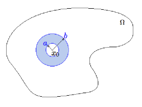
Figure 1: Domain $\Omega$.

Figure 1: Domaine $\Omega$.

Definition 1.

Assume that $\chi$ is a bump function satistying for some $k\geqslant 0$,

• $\chi\in H^{2+k}(\mathbb{R}^{d})$,
  

• $\chi_{\displaystyle{|_{\displaystyle{B(x_{0},a)}}}}=1$,
  

• $\chi_{\displaystyle{|_{\displaystyle{B(x_{0},b)^{c}}}}}=0$.

Then, with ${\bf u}_{0}:=\chi{\bf u}_{\delta}$ and $p_{0}:=\chi p_{\delta}$, we define ${\bf g}$ and $h$ as

$${\bf g}=-\mu\triangle{\bf u}_{0}+\nabla p_{0}-\delta_{x_{0}}{\bf F}\text{ and }h=\text{div }{\bf u}_{0}.$$ (6)

By the definitions of ${\bf u}_{\delta}$, $p_{\delta}$ and $\chi$, $supp({\bf g})\subset\mathcal{R}^{b}_{a}(x_{0})$ and $supp(h)\subset\mathcal{R}^{b}_{a}(x_{0})$, where $\mathcal{R}^{b}_{a}(x_{0})$ is the ring centered around $x_{0}$, of internal radius $a$ and external radius $b$, see Figure 1. Since ${\bf u}_{\delta}$ and $p_{\delta}$ are analytic on $\Omega\setminus\{x_{0}\}$, the regularity of functions ${\bf g}$ and $h$ directly depends on the regularity of function $\chi$, namely ${\bf g}\in H^{k}(\Omega)$ and $h\in H^{k+1}(\Omega)$. Finally, it only remains to correct the terms ${\bf u}_{0}$ and $p_{0}$ by solving the regular elliptic problem

$$\left\{\begin{array}[]{rccl}-\mu\triangle{\bf v}+\nabla q&=&-{\bf g}&\text{in }\Omega,\\ \text{div }{\bf v}&=&-h&\text{in }\Omega,\\ {\bf v}&=&0&\text{on }\partial\Omega,\end{array}\right.$$ (7)

and the solution of problem (4) is given by $({\bf u},p):=({\bf u}_{0}+{\bf v},p_{0}+q)=(\chi{\bf u}_{\delta}+{\bf v},\chi p_{\delta}+q),$ where ${\bf u}_{0}$ and $p_{0}$ are explicitly known functions and $({\bf v},q)$ is the solution of problem (7). Noting $({\bf v}_{h},q_{h})$ the numerical solution of problem (7) and defining ${\bf u}_{h}:={\bf v}_{h}+{\bf u}_{0}$ and $p_{h}=q_{h}+p_{0}$, we have,

$$\begin{array}[]{ll}\|{\bf u}-{\bf u}_{h}\|_{H^{s}(\Omega)}=\|{\bf v}-{\bf v}_{h}\|_{H^{s}(\Omega)},&\text{ for }0\leqslant s\leqslant k+1,\\ \|p-p_{h}\|_{H^{s}(\Omega)}=\|q-q_{h}\|_{H^{s}(\Omega)},&\text{ for }0\leqslant s\leqslant k.\end{array}$$ (8)

Actually, this method allows us to switch from the numerical computation of the solution of a singular problem with Dirac source term (with a poor convergence rate) to the numerical computation of the solution of a regular problem with an optimal convergence rate, at any required precision in terms of regularity.

3.2 Practical aspects.

For the sake of simplicity, the location of the Dirac source term will be the origin. First, we need to choose a suitable function $\chi$. Actually, to take advantage of using $P_{\ell}$-finite elements, $\ell\geqslant 1$, $\chi$ has to be $H^{\ell+1}(\mathbb{R}^{d})$, in order to ensure that ${\bf g}\in H^{\ell-1}(\Omega)$ and $h\in H^{\ell}(\Omega)$, and finally to get an optimal order of convergence. For instance, for $\ell=1$, let us define $\chi$, as a radial function, by:

$$\chi(r)=\left\{\begin{array}[]{ll}1&\text{ for }r\in[0,a],\\[2.84526pt] \displaystyle{\frac{2r^{3}-3(a+b)r^{2}+6abr+b^{2}(b-3a)}{(b-a)^{3}}}&\text{ for }r\in[a,b],\\ 0&\text{ for }r>b,\end{array}\right.$$ (9)

where the function $r$ is defined on $\mathbb{R}^{d}$ by

$$r({\bf x})=\|{\bf x}\|_{2}.$$

The function ${\bf g}$ and $h$ can be explicited. According to this definition of $\chi$, ${\bf g}$ and $h$ vanish outside the ring $a<\|{\bf x}\|_{2}<b$. For $a<\|{\bf x}\|_{2}<b$, the expressions of ${\bf g}$ and $h$ depend on the dimension,

• for $d=2$,

  $${\bf g}({\bf x}) =\frac{3}{2\pi(b-a)^{3}r}\left[\bigg{(}(3r^{2}-2(a+b)r+ab)\ln r+2r^{2}-2(a+b)r+2ab\bigg{)}{\bf I}_{2}+(ab-r^{2})\frac{{\bf x}{}^{t}{\bf x}}{r^{2}}\right]{\bf F},$$ (10)

  $$h({\bf x}) =\frac{3(1-\ln r)(r^{2}-(a+b)r+ab)}{2\pi\mu(b-a)^{3}r}{\bf x}\cdot{\bf F}.$$ (11)

• for $d=3$,

  $${\bf g}({\bf x}) =\frac{3}{4\pi(b-a)^{3}r^{2}}\left[((a+b)r-2r^{2}){\bf I}_{3}+(2ab-(a+b)r)\frac{{\bf x}{}^{t}{\bf x}}{r^{2}}\right]{\bf F},$$ (12)

  $$h({\bf x}) =\frac{3(r^{2}-(a+b)r+ab)}{2\pi\mu(b-a)^{3}r^{2}}{\bf x}\cdot{\bf F}.$$ (13)

4 Numerical illustrations.

In this section, we illustrate our theorical results by a numerical example. We define $\Omega$ as the unit square and $x_{0}=(0.5,0.5)$. The following table presents the $\mathbb{L}^{2}$-error for a direct method (dir. meth.) and a subtraction method (sub. meth.) respectively, for a characteristic mesh size $h$, and the estimated order of convergence (e.o.c.). Figure 2 illustrates the section $\{y=0.5\}$ of the error $|{\bf u}-{\bf u}_{h}|$ in the both cases. Numerical simulations evidence the fact that solving the auxiliary problem associated to the subtraction procedure of the singularity is more efficient than solving directly the problem with the Dirac source term.

$h$	$2^{-3}$	$2^{-4}$	$2^{-5}$	$2^{-6}$	$2^{-7}$	e.o.c.
Dir. meth.	$1.02\times 10^{-2}$	$4.87\times 10^{-3}$	$2.36\times 10^{-3}$	$1.21\times 10^{-3}$	$5.89\times 10^{-4}$	1.02
Sub. meth.	$4.12\times 10^{-3}$	$1.33\times 10^{-3}$	$2.92\times 10^{-4}$	$6.86\times 10^{-5}$	$2.71\times 10^{-5}$	1.88

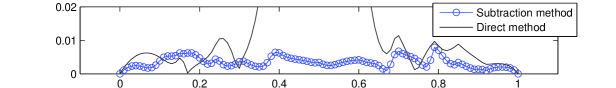
Figure 2: Section $\{y=0.5\}$ of the error $|{\bf u}-{\bf u}_{h}|$ for the direct method and the subtraction method with $h=0.125$.

Figure 2: Coupe $\{y=0.5\}$ de l’erreur $|{\bf u}-{\bf u}_{h}|$ pour la méthode directe et la méthode de soustraction avec $h=0.125$.

5 Conclusion.

To model active thin structures in a viscous fluid, such as flagella connected to bacteria or cilia involved in the mucociliary transport, we have studied Stokes problem with a singular right-hand side: a punctual force. However, when this problem is solved numerically, the singularity causes a poor convergence of the approximate solution to the exact solution. The method presented in this note preserves optimality for any approximation order, without using mesh grading. If the examples are treated with homogeneous Dirichlet conditions, the same method is still valid in the case of non homogenous Dirichlet or any affine boundary conditions (Neumann, Robin…), up to suitable adaptations. Similarly, the method can be generalized to the problem with a sum of a finite number of Dirac masses and a smooth term right-hand side.

References

- [1] R. Scott, Finite Element Convergence For Singular Data, Numerical Mathematics, 21, pp. 317-327 (1973).
- [2] T. Apel, O. Benedix, D. Sirch, B. Vexler, A Priori Mesh Grading For An Elliptic Problem With Dirac Right-Hand Side, SIAM Journal on Numerical Analysis, 49, pp. 992-1005 (2011).
- [3] P. Houston, T. P. Wihler, Discontinuous Galerkin Methods for problems with Dirac delta source, ESAIM Mathematical Modelling and Numerical Analysis, 46, pp. 1467-1483 (2012).
- [4] J. L. Lions, E. Magenes, Problèmes aux Limites Non Homogènes et Applications, 1, Dunod (1968).
- [5] C. H. Wolters, H. Köstler, C. Möller, J. Härdtlein, L. Grasedyck, W. Hackbusch, Numerical mathematics of the subtraction method for the modeling of a current dipole in EEG source reconstruction using finite element head models, SIAM Journal on Scientific Computation, 30, pp. 24-45 (2007).