Parametric description of the quantum measurement process

Abstract

We present a description of the measurement process based on the parametric representation with environmental coherent states. This representation is specifically tailored for studying quantum systems whose environment needs being considered through the quantum-to-classical cross-over. Focusing upon projective measures, and exploiting the connection between large-$N$ quantum theories and the classical limit of related ones, we manage to push our description beyond the pre-measurement step. This allows us to show that the outcome production follows from a global-symmetry breaking, entailing the observed system’s state reduction, and that the statistical nature of the process is brought about, together with the Born’s rule, by the macroscopic character of the measuring apparatus.

1 Introduction

The measurement process plays a fundamental role in any physical theory, and indeed a crucial one in quantum mechanics. The set of works dedicated to the subject is almost uncountable and different descriptions of the process often implies different interpretation of quantum mechanics itself (see for instance Refs. [1, 2] for comprehensive discussions and thorough bibliographies). The idea that measuring be a dynamical process is quite intuitive, and generally accepted. Moreover, it is today recognized that such process must include an early stage during which entanglement is generated between the observed system and the measuring apparatus, which dictates a quantum treatment for both systems. This initial stage, usually referred to as pre-measurement, can be considered successfully completed when the apparatus is in a state that conveys information on the observed system, a condition related with the occurrence of decoherence[3, 2]. We usually take what happens next from the measurement postulate, although whether or not its content can be derived from the other postulates is still the most debated issue of quantum theory [4, 5, 1, 6, 7, 3, 2, 8].

In this work, embodying the formal definition of the large-$N$ limit of a quantum theory[9] into the parametric representation with environmental coherent states (PRECS)[10, 11, 12], we complement the description of the measurement process with the quantum-to-classical cross-over of the apparatus only. We thus manage to understand how objective results emerge from the entangled states of a macroscopic measuring apparatus, and why their production is an inherently statistical phenomenon. The observed system’s state reduction and the Born’s rule are contextually obtained.

The structure of the paper is as follows: We first introduce the standard model for unitary pre-measurements [4, 1, 8] and study its dynamics by the PRECS. The condition that defines the successful completion of the pre-measurement is then formally expressed[13], and two paradigmatic models (spin-$\frac{1}{2}$ in either a bosonic or a magnetic environment) are introduced, in order to clarify the formalism and guide the interpretation. At this point we formally associate the classical limit of the environment to the macroscopic character of the measuring apparatus referring to the seminal work by L.G.Yaffe[9] on large-$N$ quantum theories; this finally allows us to describe the outcome production. In order to ease the understanding of our proposal, we keep comments to a minimum throughout its presentation, and postpone them to the concluding section.

2 Pre-measurement and parametric representation

Let us first outline the formalism to which we will essentially refer in describing the quantum measurement process. Be $\Gamma$ the observed quantum system (with Hilbert space ${\cal H}_{\Gamma}$), and $\Xi$ the measuring apparatus (with Hilbert space ${\cal H}_{\Xi}$). The composite system $\Psi{{=}}\Gamma{+}\Xi$ is assumed isolated, i.e. $\rho_{\Psi}(t){{=}}|{\Psi(t)}\rangle\langle{\Psi(t)}|$, at any time prior to the output production ($t{<}T$); moreover its state is taken separable before the measurement starts ($t{\leq}0$)

$$|{\Psi(t\leq 0)}\rangle=|{\Gamma}\rangle\otimes|{\Xi}\rangle~{}.$$ (1)

Note that the validity of these assumptions should not be taken for granted, as extensively discussed in Refs.[1, 2].

Let us concentrate upon sharp observables, defined as - and identified with - projection operator valued measures on the real Borel space, or a subset of it[1]. Any such measure, $O_{\Gamma}$, determines a unique Hermitian operator $\hat{O}_{\Gamma}$ acting on ${\cal H}_{\Gamma}$; if the observable is further assumed (for the sake of clarity) discrete and non-degenerate, it is $\hat{O}_{\Gamma}{=}\sum_{\gamma}\omega_{\gamma}|{\gamma}\rangle\langle{\gamma}|$, and the $\hat{O}_{\Gamma}$-eigenvectors $\{|{\gamma}\rangle\}_{{\cal H}_{\Gamma}}$ form an orthonormal basis for ${\cal H}_{\Gamma}$. Further ingredients of a scheme designed for describing the measure of $O_{\Gamma}$ are i) a pointer observable $O_{\Xi}$ of $\Xi$, ii) a pointer function correlating the value sets of $O_{\Xi}$ and $O_{\Gamma}$, iii) a measurement coupling between $\Gamma$ and $\Xi$, ultimately responsible for the $\Psi$-state transformation $\rho_{\Psi}(0)\xrightarrow{V}\rho_{\Psi}(t)$ occurring before the actual production of a specific output is obtained. It can be shown that a sufficient condition for a state transformation to qualify as a proper pre-measurement[1], is that $V$ be a trace-preserving linear mapping. When $V$ is further assumed to be unitary, the process coincides with the one first described by von Neumann[4], later generalized by several authors [14, 15, 16, 17], and characterized by Ozawa[18] under the name of conventional measuring process. If $O_{\Xi}$ is a sharp observable, with $\hat{O}_{\Xi}$ the corresponding hermitian operator, choosing $V{=}e^{-it\hat{H}_{\Psi}}$ with

$$\hat{H}_{\Psi}=u\,\hat{O_{\Gamma}}\otimes\hat{O_{\Xi}}+\hat{{\rm I\!I}}_{\Gamma}\otimes\hat{H}_{\Xi}~{},$$ (2)

defines the standard model[1] for describing pre-measurements as dynamical processes, where $\hat{H}_{\Xi}$ acts on ${\cal H}_{\Xi}$, $\hat{{\rm I\!I}}_{\Gamma}$ is the identity operator on ${\cal H}_{\Gamma}$, and we have set $\hbar{=}1$. In what follows we will specifically study the above standard model, taking the identity as the pointer function, for the sake of simplicity. Writing $|{\Gamma}\rangle$ in Eq. (1) on the basis of the $\hat{O}_{\Gamma}$-eigenstates, from Eq. (2) it follows

$$|{\Psi(t)}\rangle=\sum_{\gamma}c_{\gamma}|{\gamma}\rangle\otimes|{\Xi^{\gamma}(t)}\rangle~{}$$ (3)

at any time during the pre-measurement ($0{<}t{<}T$), with

$$|{\Xi^{\gamma}(t)}\rangle\equiv e^{-it\hat{H}^{\gamma}_{\Xi}}|{\Xi}\rangle~{},$$ (4)

and

$$\hat{H}^{\gamma}\equiv u\,\omega_{\gamma}\hat{O}_{\Xi}+\hat{H}_{\Xi}~{}.$$ (5)

In the standard model, the possibility of extracting information about $\Gamma$ reporting on $\Xi$, relies on the $\gamma$-dependence of $|{\Xi^{\gamma}(t)}\rangle$, i.e. on the dynamical entanglement generation induced by the coupling $u\hat{O}_{\Gamma}\otimes\hat{O}_{\Xi}$ if, and only if, $|{\Xi}\rangle$ is not a $\hat{O}_{\Xi}$-eigenstate. On the other hand, the measuring apparatus is expected to be in a stationary state before the above coupling is switched on. Therefore, it is usually taken

$$\hat{H}_{\Xi}|{\Xi}\rangle=E_{0}|{\Xi}\rangle~{}~{}~{}{\rm and}~{}~{}~{}[\hat{O}_{\Xi},\hat{H}_{\Xi}]\neq 0~{}.$$ (6)

The evolution described by Eq. (3) can be studied by the PRECS[11], a method based on the use of generalized coherent states [19, 20, 21] for $\Xi$, whose construction, as far as the model (2) is concerned, can be summarized as follows. Consider the operators $\hat{O}_{\Xi}$ and $\hat{H_{\Xi}}$: they will generally be elements of a Lie group $G$, usually dubbed (environmental) dynamical group, and, in most physical situation, they also belong to the related Lie algebra g (in that they are linear combination of the group generators). The arbitrary choice of a reference state $|{R}\rangle{\in}\mathcal{H}_{\Xi}$ defines the subgroup $F$ of the operators $\hat{f}$ acting trivially on $|{R}\rangle$, i.e. such that $\hat{f}|{R}\rangle{=}e^{i\phi_{f}}|{R}\rangle$, and hence the environmental coset $G/F$. Environmental coherent states (ECS) are the states

$$|{\Omega}\rangle=\hat{\Omega}|{R}\rangle~{}{\rm with}~{}\hat{\Omega}\in G/F~{}.$$ (7)

It is demonstrated[19, 20, 21] that coherent states $|{\Omega}\rangle$ are in one-to-one correspondence with points $\Omega$ on a differentiable manifold ${\cal M}$. The construction of ECS entails the definition of an invariant (with respect to $G$) measure $d\mu(\Omega)$ on ${\cal M}$, as well as of a metric tensor ${\bf m}$. Moreover, ECS form an over-complete set on ${\cal H}_{\Xi}$, and provide an identity resolution in the form

$$\hat{{\rm I\!I}}_{\Xi}=\int_{\cal M}\,d\mu(\Omega)|{\Omega}\rangle\langle{\Omega}|~{},$$ (8)

where $\hat{\rm I\!I}_{\Xi}$ is the identity operator on ${\cal H}_{\Xi}$. Getting back to the model (2), if g is semi-simple, referring to its Cartan basis , and reminding condition (6), one recognizes that $\hat{H}^{\gamma}$ is in the canonical form with $\hat{O}_{\Xi}$ hermitian linear combination of shift-up and -down operators : This usually entails the choice of $|{R}\rangle$ as the eigenstate of $\hat{H}_{\Xi}$ such that $\hat{O}_{\Xi}|{R}\rangle{{=}}0$, that naturally provides ${\cal M}$ with a symplectic structure [22, 23], i.e. ${\Omega}{=}(z,\bar{z})$ with $z,\bar{z}$ canonical coordinates, and $d\mu(\Omega){{=}}{\rm det}({\bf m})dzd\bar{z}$. Consistently with conditions (6), we can set $|{\Xi}\rangle{=}|{R}\rangle$, implying

$$\langle{\Xi|\hat{O}_{\Xi}|\Xi}\rangle=0~{}.$$ (9)

Coherent states have peculiar dynamical properties, which are often summarized by the motto ”once a coherent state, always a coherent state”[19]. In the specific case of a system ruled by the Hamiltonian (2), with initial state (1), these properties, complemented with the choice $|{R}\rangle{{=}}|{\Xi}\rangle$, allows one to write[11]

$$|{\Xi^{\gamma}(t)}\rangle=e^{i\varphi^{\gamma}_{t}}|{\Xi^{\gamma}_{t}}\rangle~{},$$ (10)

where $|{\Xi^{\gamma}_{t}}\rangle$ is the coherent state corresponding to the point ${\Xi}^{\gamma}(t)$ along the trajectory on ${\cal M}$ defined by the solution of the classical-like equations of motion

$$i{\rm m}_{z\bar{z}}\frac{dz}{dt}=\frac{\partial}{\partial\bar{z}}H^{\gamma}(\Omega)~{},~{}{\rm and~{}the~{}same~{}with}~{}z\leftrightarrow\bar{z}~{},\$$ (11)

with $H^{\gamma}(\Omega){\equiv}\langle{\Omega|\hat{H}^{\gamma}|\Omega}\rangle$ and $\Xi^{\gamma}(0){{=}}0$; as for the phase factor it is $\varphi^{\gamma}_{t}{{=}}\int_{0}^{t}~{}dy~{}\langle{\Xi^{\gamma}_{y}|\left(i\frac{\partial}{\partial y}-\hat{H}^{\gamma}\right)|\Xi^{\gamma}_{y}}\rangle$.

Once the ECS are constructed, any state of the composite system $\Psi$ can be parametrically represented by formally splitting $\Gamma$ and $\Xi$ through the insertion of $\hat{\rm I\!I}_{\Xi}$ in the form (8), as shown in Ref. [10]. In particular, exploiting the fact that $d\mu(\Omega)$ is group-invariant, the state (3) reads

$$|{\Psi(t)}\rangle=\int_{\cal M}\,d\mu(\Omega)\chi_{t}(\Omega)~{}|{\phi_{t}(\Omega)}\rangle\otimes|{\Omega}\rangle~{},$$ (12)

with

$$|\phi_{t}(\Omega)\rangle=\frac{1}{\chi_{t}(\Omega)}\sum_{\gamma}c_{\gamma}\langle{\Omega|\Xi^{\gamma}(t)}\rangle~{}|{\gamma}\rangle~{},$$ (13)

$$\chi^{2}_{t}(\Omega)=\sum_{\gamma}|c_{\gamma}|^{2}h^{\gamma}_{t}(\Omega)~{}~{},~{}~{}h^{\gamma}_{t}(\Omega)=|\langle{\Omega|\Xi^{\gamma}_{t}}\rangle|^{2}~{},$$ (14)

and we have set $\chi_{t}(\Omega)$ in $R^{+}$ by choosing its arbitrary phase equal to $0$. Equations (12-14) define the parametric representation with ECS of $|{\Psi(t)}\rangle$. Notice that the dependence of the principal system’s pure states $|{\phi_{t}(\Omega)}\rangle$ on $\Omega$ is the signature that $\Gamma$ and $\Xi$ are entangled[10]. Moreover, due to $\langle{\Psi(t)|\Psi(t)}\rangle{{=}}1$, it is $\int_{\cal M}d\mu(\Omega)\chi^{2}_{t}(\Omega){{=}}1$ at any time, which allows one to interpret $\chi^{2}_{t}(\Omega)$ as the normalized density distribution of ECS on the manifold ${\cal M}$ [19, 10].

3 Informative apparatus

The essential goal of any pre-measurement is that of setting a cogent relation between elements of $\{|{\gamma}\rangle\}_{{\cal H}_{\Gamma}}$ and pointer states[24] of the measuring apparatus. Referring to Eq. (3), this implies that

$$\!\!\!\!\!\!\!\!\!\!\!\!\!\!\!\!\!\!\!\!\!\!\!\!\!\!\!\!\!\!\!\!\!{\rm different~{}states}~{}|{\Xi^{\gamma}(\tau)}\rangle~{}{\rm and}~{}|{\Xi^{\gamma^{\prime}}(\tau)}\rangle~{},$$ (15)

$$\!\!\!\!\!\!\!\!\!\!\!\!\!\!\!\!\!\!\!\!\!\!\!\!\!\!\!\!\!\!\!\!\!{\rm produce~{}different~{}outcomes~{}whenever}~{}\gamma\neq\gamma^{\prime}~{},$$ (16)

for $\tau{>}\tau_{\rm d}$, where $\tau_{\rm d}$ is the time when the pre-measurement can be considered successfully concluded. Condition (15-16) can be translated[13] into some property that $\chi^{2}_{\tau}(\Omega)$ must feature in order to describe an informative apparatus: in fact, defining the $\varepsilon$-support of each component $h^{\gamma}_{t}(\Omega)$ as the region ${\cal S}^{\gamma}_{t}{\in}{\cal M}$ such that $h^{\gamma}_{t}(\Omega){>}\varepsilon~{}\forall\Omega{\in}{\cal S}^{\gamma}_{t}$, with $\varepsilon$ a small number in $R^{+}$, the request (15-16) can be identified[13] with the condition

$${\cal{S}}^{\gamma}_{\tau}\cap{\cal{S}}^{\gamma^{\prime}}_{\tau}=\emptyset~{}~{}{\rm for}~{}~{}\gamma\neq\gamma^{\prime}~{}.$$ (17)

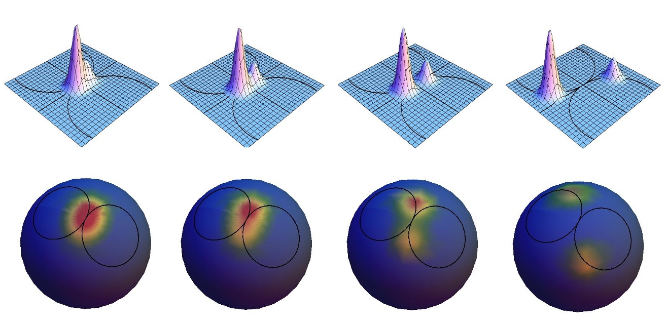
Figure 1: Evolution of $\bar{\chi}^{2}_{t}(\Omega)$ for the models (19) and (20), top and bottom panels, respectively, as time goes by from left to right. Black lines indicate the trajectories $\Xi^{\gamma}_{t}$, with $\gamma{=}\pm$.

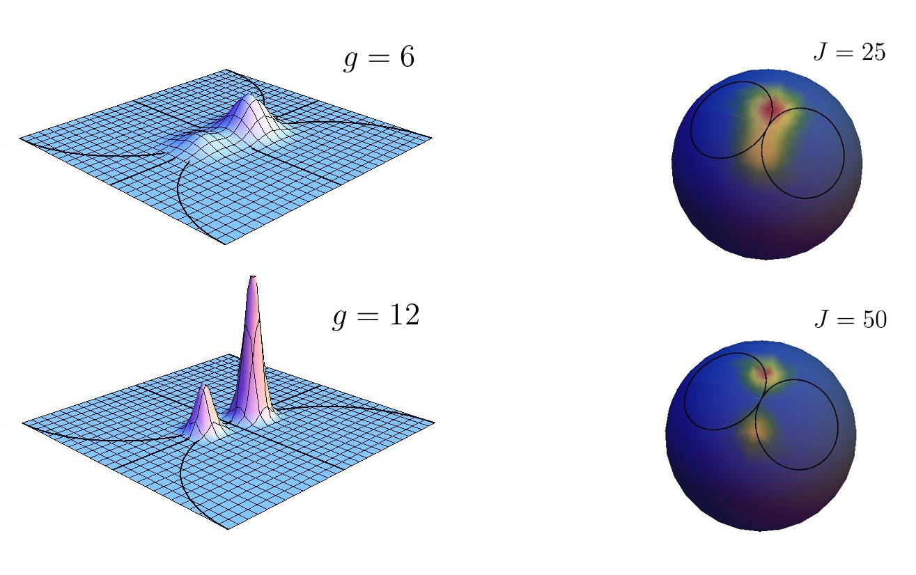
Figure 2: $\bar{\chi}^{2}_{t}(\Omega)$ at a given time for the models (19) and (20) with different parameters $g$ and $J$ - left and right panels respectively - Black lines as in Fig.1.

The one-to-one correspondence thus established between each function $h^{\gamma}_{\tau}$ and the region ${\cal S}^{\gamma}_{\tau}$ in ${\cal M}$ allows one to write

$$|{\Psi(\tau)}\rangle=\sum_{\gamma}c_{\gamma}\!\int_{{\cal S}^{\gamma}_{\tau}}\,d\mu(\Omega)e^{i\varphi^{\gamma}_{t}}\sqrt{h^{\gamma}_{\tau}(\Omega)}~{}\,|{\gamma}\rangle\otimes|{\Omega}\rangle~{}$$ (18)

for all $\tau$ in the time interval where condition (17) holds. Notice that, despite such condition specifically concern the apparatus, Eq. (18) strictly implies that decoherence with respect to the basis $\{|{\gamma}\rangle\}_{{\cal H}_{\Gamma}}$ has occurred[25, 13], and the time $\tau_{\rm d}$ is consistently recognized as a decoherence time for $\Gamma$. For the sake of a lighter notation we will hereafter drop the $\tau$ index in ${\cal S}^{\gamma}_{\tau}$ understanding that, whenever ${\cal S}^{\gamma}$ is referred to, it is $\tau{>}\tau_{\rm d}$. For a more transparent discussion, it is now worth considering two models with Hamiltonian of the form $(\ref{e.H})$, that have been introduced as paradigmatic ones for describing the decoherence phenomenon, and extensively studied in various contexts [2, 26]. They are described by

$$\hat{H}_{qb}=\nu\hat{b}^{\dagger}\hat{b}+g\hat{\sigma}^{z}\otimes(\hat{b}+\hat{b}^{\dagger})~{},$$ (19)

and

$$\hat{H}_{qS}=h\hat{J}^{z}+\mu\hat{\sigma}^{z}\otimes\hat{J}^{x}~{},$$ (20)

where $\hat{\sigma}^{z}$ is the $Z$-Pauli matrix, $\hat{b}$ and $\hat{b}^{\dagger}$ are bosonic operators ($[\hat{b},\hat{b}^{\dagger}]{=}1$), and $\hat{J}^{\pm}{=}\hat{J}^{x}\pm i\hat{J}^{y}$ are spin-$J$ operators ($[\hat{J}^{\alpha},\hat{J}^{\beta}]{=}i\varepsilon^{\alpha\beta\gamma}\hat{J}^{\gamma}$). The respective ECS are those usually referred to as field and spin coherent states, with $|{R}\rangle$ such that $\hat{b}|{R}\rangle{=}0$ and $\hat{J}^{-}|{R}\rangle{=}0$, and manifold $\cal M$ the complex plane and the unit $2$-sphere. The trajectories ${\Xi}^{\gamma}_{t}$ defining the states $|{\Xi^{\gamma}_{t}}\rangle$ in Eqs. (13-14), with $\gamma{=}\pm$, can be explicitly determined [25] and are shown in Fig.1 as black lines on the respective manifold. In the same figure, the distributions $\bar{\chi}^{2}_{t}(\Omega){\equiv}{\rm det}({\bf m})\chi^{2}_{t}(\Omega)$ are plotted at various times: it strikes that, as time goes by, they acquire a multi-modal structure, with as many distinct modes as the number of different $\gamma$ in the $\hat{O}_{\Gamma}$-spectrum, thus visualizing how condition (17) is dynamically achieved. Moreover, considering $\bar{\chi}^{2}_{t}(\Omega)$ for different values of $g$ and $J$, as in Fig. 2, reveals that when such parameters increase, each $\gamma$-peak becomes more pronounced, and the corresponding support ${\cal{S}^{\gamma}}$ consequently shrinks around ${\Xi}^{\gamma}_{t}$. This evidence, that reflects the more general result[9] briefly stated at point ii) of the next section, is clearly reminiscent of some sort of classical limit for $\Xi$. The description of the process which is now available allows us to push the formalism towards a well defined macroscopic limit for the measuring apparatus only, that leave the principal system unaffected.

4 Large-N limit

This Section is based on a work by L.G.Yaffe[9], dealing with the fundamental question “Can one find a classical system whose dynamics is equivalent to some $N\rightarrow\infty$ limit of a given quantum theory?”, where $N$ is some measure of the number of dynamical variables. An extensive discussion of Ref. [9] goes beyond the scope of this letter, but briefly retracing the reasoning underlying the results which are most relevant to get to our final goal, is necessary. In doing that we will try to keep contact with what we have described so far.

Given that:

- a classical theory, $C$, is defined by a phase space $\cal C$, a Poisson bracket, and a classical Hamiltonian $H_{\rm cl}$;

- a quantum theory, $Q$, is defined by a Hilbert space, a Lie algebra, and a Hamiltonian $\hat{H}$ (and dynamical group $G$),

then:

i) Be $Q_{\kappa}$ a quantum theory characterized by some (quanticity) parameter $\kappa$, assumed to take positive real values including the limiting $\kappa{=}0$ one. This is the theory that describes the apparatus $\Xi$ in the above sections, in particular, $\kappa{=}1/g$ or $1/J$ in the models (19) or (20), respectively.

ii) It exists a minimal set of conditions that $Q_{\kappa}$ must fulfill to guarantee that its $\kappa\to 0$ limit is a classical theory $C$. Such conditions emerge in terms of coherent states for the dynamical group of the theory, $G_{\kappa}$, and establish a one-to-one correspondence, ${\cal M}_{\kappa}\to{\cal C}$, between points on the related manifold and on the phase-space of $C$. These coherent states are the ECS defined in the previous section, and one of the above conditions implies

$$h^{\gamma}_{t}(\Omega){\rm det}({\bf m})~{}~{}\underset{\kappa\to 0}{\longrightarrow}~{}~{}\delta(\Omega-\Xi^{\gamma}_{t})~{},$$ (21)

as suggested in Fig. 2.

iii) Be $Q_{N}$ a quantum many-body (field) theory with some global $X(N)$ symmetry ($X{=}O,Sp,U$…), dynamical group $G_{N}$, and related manifold ${\cal M}_{N}$. This is the microscopic quantum theory that would exactly describe the apparatus $\Xi$, were we able to determine the details of its internal interactions as well as of those between each one of its components and $\Gamma$.

iv) Any such $Q_{N}$ theory defines a $Q_{\kappa}$ one, by this meaning that the latter can be explicitly defined from the former, such that $\kappa{=}1/N$ (or $1/N^{2}$, depending on specific features of $Q_{N}$). The relation between the two theories is established via their respective dynamical groups, $G_{N}$ and $G_{\kappa}$, by making them be different representations of the same algebra. Operators $\hat{A}_{\kappa}$ and $\hat{A}_{N}$ in the two different theories are also formally related (though it is not possible to explicitly express such relation in general).

v) It is demonstrated that $\lim_{N\to\infty}Q_{N}{=}\lim_{\kappa\to 0}Q_{\kappa}{=}C$, where the last equality means that $Q_{\kappa}$ fulfills the conditions of point ii) as $\kappa\to 0$. The above chain of equalities implies the existence of a mapping from ${\cal M}_{N}\to{\cal M}_{\kappa}\to{\cal{C}}$, with the last correspondence biunivocal, as from point ii).

Resulting from the above is the following: to each $|{\Omega}\rangle$, coherent state for $Q_{\kappa}$, it is associated a set $\{|{\Omega\scriptscriptstyle{N}}\rangle\}_{\sim}$ of coherent states for $Q_{N}$ such that

$$\lim_{N\to\infty}\langle{\Omega{\scriptscriptstyle{N}}_{i}|\hat{A}_{N}|\Omega{\scriptscriptstyle{N}}_{i}}\rangle=\lim_{k\to 0}\langle{\Omega|\hat{A}_{\kappa}|\Omega}\rangle{\equiv}A_{\rm cl}(\Omega)~{},$$ (22)

for all $|{\Omega\scriptscriptstyle{N}_{i}}\rangle{\in}\{|{\Omega{\scriptscriptstyle{N}}}\rangle\}_{\sim}$ and any hermitian operator $\hat{A}_{\kappa}$ with $A_{\rm cl}(\Omega){<}\infty$. Elements of the same set are related by $|{\Omega{\scriptscriptstyle{N}}_{i}}\rangle{=}{\cal U}_{ij}|{\Omega{\scriptscriptstyle{N}}_{j}}\rangle$ with ${\cal U}_{ij}$ any unitary $X(N)$-symmetry operation. Operators $\hat{A}_{\kappa}$ and $\hat{A}_{N}$ are related as from point iv), and $A_{\rm cl}$ is a real function on $\cal C$, with $A_{\rm cl}(\Omega)$ its value on the point that univocally corresponds to $|{\Omega}\rangle$, according to point ii). Verbalizing Eq. (22), states in $\{|{\Omega{\scriptscriptstyle{N}}}\rangle\}_{\sim}~{}$ are dubbed classically equivalent, and operators such that their symbols $\langle{\Omega{\scriptscriptstyle{N}}|\cdot|\Omega{\scriptscriptstyle{N}}}\rangle$, keep finite for $N\to\infty$ are called classical operators[9].

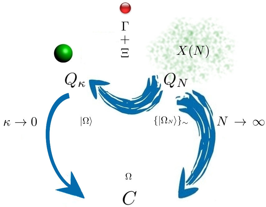
Figure 3: Graphical depiction of the relation between effective and microscopic theories, $Q_{\kappa}$ and $Q_{N}$, giving rise to the same classical theory $C$.

5 Macroscopic measuring apparatus

Regarding the measurement process, Yaffe’s results teaches us that the classical limit ($\kappa\to 0$) of the effective theory $Q_{\kappa}$ used for describing $\Xi$ during the pre-measurement, can keep describing a macroscopic ($N\to\infty$) apparatus; however, in order for this to be the case, an $X(N)$-invariant $Q_{N}$ theory must actually underlie $Q_{\kappa}$, being the one that would provide us with the exact, microscopic description of $\Xi$, if we were able to deal with it in the large-$N$ limit.

We can now get back to the PRECS treatment, to find that the theory $Q_{\kappa}$, with its related coherent states $|{\Omega}\rangle$, is already well defined, and the symbols $\langle{\Omega|\hat{A}_{k}|\Omega}\rangle$ are the Husimi functions[19, 20, 21] of operators acting on ${\cal H}_{\Xi}$. Therefore, from condition (17) and Eq. (22), we find that to each $\cal{S}^{\gamma}$, and hence to each trajectory in ${\cal M}$, it corresponds a set $\{|{\Omega{\scriptscriptstyle{N}}}\rangle\}^{\gamma}_{\sim}$ of classically equivalent coherent states of the microscopic, $X(N)$-invariant, quantum theory $Q_{N}$.

States belonging to the same set $\{|{\Omega{\scriptscriptstyle{N}}}\rangle\}^{\gamma}_{\sim}$ keep being distinct in the large-$N$ limit, as this limit does not affect the transformations ${\cal U}_{ij}$ that relate them. Therefore, the set ${\cal V}^{\gamma}_{N}$ of points corresponding to $\{|{\Omega{\scriptscriptstyle{N}}}\rangle\}^{\gamma}_{\sim}$ in ${\cal M}_{N}$ has a finite volume $V^{\gamma}_{N}$ even if the apparatus becomes macroscopic.

States belonging to sets $\{|{\Omega{\scriptscriptstyle{N}}}\rangle\}^{\gamma}_{\sim}$ labeled by different $\gamma$s are related by

$$|{\Omega{\scriptscriptstyle{N}_{i}}(t)}\rangle^{\!\gamma^{\prime}}=U^{\gamma\gamma^{\prime}}_{N}(t)|{\Omega{\scriptscriptstyle{N}_{i}}(t)}\rangle^{\!\gamma}$$ (23)

$$\!\!\!\!\!\!\!\!\!\!\!\!\!\!{\rm with~{}~{}~{}} U^{\gamma\gamma^{\prime}}_{N}(t)\equiv e^{-it\hat{H}^{\gamma^{\prime}}_{N}+it\hat{H}^{\gamma}_{N}}~{},$$ (24)

which follows from the fact that evolutions defined by different $\gamma$s have the same initial state. For $t{{>}}\tau_{\rm d}$ they are not classically equivalent, implying ${\cal V}^{\gamma}_{N}\cap{\cal V}^{\gamma^{\prime}}_{N}{=}\emptyset$, but yet they have the same energy in the $N\to\infty$ limit,

$$\!\!\!\!\!\!\!\!\!\!\!\!\!\!\!\!\lim_{N\to\infty}\langle{\Omega{\scriptscriptstyle{N}}|\hat{H}^{\gamma}_{N}|\Omega{\scriptscriptstyle{N}}}\rangle\underset{\Omega{\scriptscriptstyle{N}}\in\cup_{\gamma}{\cal V}^{\gamma}_{N}}{=}$$ (25)

$$\!\!\!\!\!\!\!\!\!\!\!\!\!\!\!\!\lim_{\kappa\to 0}\langle{\Omega|\hat{H}^{\gamma}|\Omega}\rangle\underset{\Omega\in\cup_{\gamma}{\cal S}^{\gamma}}{=}H_{\rm cl}(\Xi^{\gamma}_{\tau})=E_{0}~{},$$ (26)

as seen from Eqs.  (22), (21), (9), and (6).

The above analysis tells us that if one were to study the behaviour of a macroscopic measuring apparatus in terms of its microscopic quantum theory, despite not being able to do it exactly due to the large number of dynamical variables, yet she could extract information on $\Xi$, for $t{{>}}\tau_{\rm d}$ and $N\to\infty$, from the degenerate coherent states $\cup_{\gamma}\{|{\Omega{\scriptscriptstyle N}}\rangle\}^{\gamma}_{\sim}$, grouped into disjoint sets of classically equivalent ones.

6 Outcome production

Suppose now that, at a certain time $T{>}\tau_{\rm d}$, a local perturbation acts on some parts of $\Xi$, thus breaking the global $X(N)$-symmetry. The relation between $Q_{N}$ and $Q_{\kappa}$ is consequently broken, and the latter theory cannot be further used for describing the apparatus. The only tool with which we are left for studying $\Xi$ is the microscopic theory $Q_{N}$, and the information collected upon it in the previous section. According to the usual description of symmetry breaking (SB) in systems made by a large number of particles, and exclusively focusing upon the $N\to\infty$ limit of $Q_{N}$, the above $X(N)$-SB will select some states amongst those that equivalently describe the measuring apparatus immediately before $T$, by making their energy lower than that of all the others. Specifically, as the operator $\hat{\delta}$ representing the local SB-perturbation cannot commute with any of the global transformations $\hat{U}^{\gamma\gamma^{\prime}}_{N}$ in Eqs. (23-24), neither can it depend on the spectrum $\{\omega_{\gamma}\}$, it is ${}^{\gamma}\!\langle{\Omega{\scriptscriptstyle{N}_{i}}|\,\hat{\delta}\,|\Omega{\scriptscriptstyle{N}_{i}}}\rangle^{\!\gamma}{\neq}^{\gamma^{\prime}}\!\!\langle{\Omega{\scriptscriptstyle{N}_{i}}|\,\hat{\delta}\,|\Omega{\scriptscriptstyle{N}_{i}}}\rangle^{\!\gamma^{\prime}}$ unless they both vanish. In other terms, a local perturbation on $\Xi$ that be independent on the previous evolution of $\Psi$, cannot cause the same energy-lowering in states belonging to different sets of classically equivalent coherent states.

Therefore, only one $\gamma_{\rm out}$ will be selected

$$\cup_{\gamma}\{|{\Omega{\scriptscriptstyle{N}}}\rangle\}^{\gamma}_{\sim}~{}~{}~{}\underset{X(N){\text{-}{\rm SB}}}{-\!\!-\!\!-\!\!-\!\!-\!\!\longrightarrow}~{}~{}~{}\{|{\Omega{\scriptscriptstyle{N}}}\rangle\}^{\gamma_{\rm out}}_{\sim}~{}.$$ (27)

Picking one specific set of classically equivalent coherent states, i.e. one specific $\gamma_{\rm out}$, ensures that all classical functions get their respective definite value $A_{\rm cl}(\Xi^{\gamma_{\rm out}}_{T})$ on the classical phase-space ${\cal C}$ via Eq. (22), and a classical behaviour unambiguously emerges for the measuring apparatus. In particular, the classical function corresponding to $\hat{O}_{\Xi}$ will take the value $O_{\rm cl}(\Xi^{\gamma_{\rm out}}_{T})$, which will be the result of the measurement process.

Notice that the effective theory describing the apparatus during the pre-measurement is $X(N)$-symmetric if and only if the interaction between $\Gamma$ and $\Xi$ also features such symmetry; therefore, the $X(N)$-SB is only made possible by the outwards opening of $\Psi$, i.e. by enlarging the system considered during the pre-measurement from $\Psi{=}\Gamma+\Xi$ to $W{=}\Psi+R$, where by $R$ we mean the ”rest of the world”. The action of $R$ on $\Xi$ can be controlled, just like in an actual measurement where it is triggered by the reading of the apparatus. It can also be completely random, in which case the $X(N)$-SB induces the emergence of classicality. Whatever the situation, such action is uncorrelated with the dynamics of $\Psi$ before the symmetry breaking.

7 Born’s rule

In order to understand what value of $\gamma_{\rm out}$ one should in principle expect, let us go back to our measuring apparatus after the pre-measurement is concluded but before the SB has occurred ($\tau_{\rm d}{<}\tau{<}T$): In previous sections we have learned that its macroscopic ($N\to\infty$) behaviour follows from the features of the ensemble $\{\{|{\Omega{\scriptscriptstyle{N}}}\rangle\}^{\gamma_{1}}_{\sim},\{|{\Omega{\scriptscriptstyle{N}}}\rangle\}^{\gamma_{2}}_{\sim},...\}$ of degenerate coherent states, grouped into disjoint sets, each labeled by a specific $\gamma$. States belonging to the same set correspond, as $N\to\infty$ and at any time $\tau{>}\tau_{\rm d}$, to the same point $\Xi^{\gamma}_{\tau}$ in ${\cal C}$, and hence to the same possible outcome $O_{\rm cl}(\Xi^{\gamma}_{T})$. On the other hand, due to degeneracy and to the fact that the perturbation causing the $X(N)$-SB is uncorrelated with the evolution of the overall system $\Psi$, states belonging to the above ensemble are all equally likely. Therefore, the principles of statistical mechanics tell us that the probability $p(\gamma_{\rm out})$ of the outcome $O_{\rm cl}(\Xi^{\gamma_{\rm out}}_{T})$ is proportional to the volume $V^{\gamma}_{N}$ occupied by the set ${\cal V}^{\gamma_{\rm out}}_{N}$ of representative points in ${\cal M}_{N}$, at $\tau{=}T$ and as $N\to\infty$. Being left with the final problem of evaluating $V^{\gamma}_{N}$, we consider the following: prior to the symmetry breaking, the two theories $Q_{N}$ and $Q_{\kappa}$, in their respective large-$N$ and $\kappa\to 0$ limit, describe the same classical behaviour of $\Xi$. Therefore, getting back to $\Psi{=}\Gamma+\Xi$, for $\tau{>}\tau_{\rm d}$ it is

$$\langle{\Psi|{\mathbb{I}}_{\cal{H}_{\gamma}}\otimes\hat{A}|\Psi}\rangle=\sum_{\gamma}\int_{\cal{S}_{\gamma}}d\mu(\Omega)\chi^{2}_{\tau}(\Omega)\langle{\Omega|\hat{A}|\Omega}\rangle$$ (28)

and it must be

$$\lim_{\kappa\to 0}\langle{\Psi|{\mathbb{I}}_{\cal{H}_{\gamma}}\otimes\hat{A}|\Psi}\rangle=\lim_{N\to\infty}\sum_{\gamma}\int_{{\cal V}^{\gamma}_{N}}d\mu(\Omega{\scriptscriptstyle{N}})\langle{\Omega{\scriptscriptstyle{N}}|\hat{A}_{N}|\Omega{\scriptscriptstyle{N}}}\rangle$$ (29)

for any classical operator $\hat{A}$ acting on ${\cal H}_{\Xi}$, and for all initial states $|{\Gamma}\rangle$ (i.e. for all possible sets of $\{c_{\gamma}\}$ such that $\sum_{\gamma}|c_{\gamma}|^{2}{=}1$). Given Eq. (22) this is seen to require

$$V^{\gamma}_{N}\propto \lim_{N\to\infty} \int_{{\cal V}^{\gamma}}d\mu(\Omega{\scriptscriptstyle{N}})$$ (30)

$$= \lim_{\kappa\to 0} \int_{\cal{S}^{\gamma}}d\mu(\Omega)\chi^{2}_{\tau}(\Omega){=}|c_{\gamma}|^{2}~{},$$ (31)

which results in the Born’s rule

$$p(\gamma_{\rm out})=|c_{\gamma^{\rm out}}|^{2}~{}.$$ (32)

Finally notice that the selection entailed by Eq. (27) trails behind itself that of the state $|{\gamma_{\rm out}}\rangle$ for $\Gamma$, as seen from Eqs. (13) and (21), thus realizing the reduction of the observed system’s quantum state.

Before moving towards some concluding comments, we note that considering degenerate, possibly continuous, sharp observables and/or non trivial pointer functions is just a matter of a more complicated notation. On the other hand, the generalization to un-sharp observables, i.e. POVM rather than projective measurements, is a more delicate issue, that will be possibly tackled in future works.

8 Conclusions

Let us briefly retrace the route that brought us from the initial separable state $|{\Gamma}\rangle\otimes|{\Xi}\rangle$ to the production of an outcome, and the Born’s rule.

We have considered projective measures and, referring to the standard model of unitary pre-measurements, analyzed their dynamics by means of some specific tools, namely generalized coherent states and the PRECS. After having expressed the necessity of decoherence as a condition on the distribution of quantum states relative to the apparatus, we have formally substantiated the intuitive relation between

(1)

the classical limit of the effective quantum theory used in the standard model for describing the apparatus by a limited number of dynamical variables, and

(2)

the large-$N$ limit of the microscopic theory that would exactly describe, were we able to handle it, a macroscopic quantum measuring apparatus.

This has enlightened that a global symmetry must characterize (2) if (1) is to be given a physical meaning: In fact, the breaking of such symmetry causes the breakdown of the effective quantum description of the apparatus adopted during the pre-measurement and contextually selects an objective outcome. The fact that a huge number of microscopic configurations of the apparatus correspond to the same outcome brings probabilities into play, according to the principles of statistical mechanics and with no consequences on the deterministic nature of the quantum description. In other terms, observing a quantum system with a macroscopic apparatus produces a probabilistic result not due to the system being quantum but rather because the apparatus is big.

The reader will recognize, all along the description proposed in this work, many concepts and formal elements characterizing previous approaches to the quantum measurement process, from einselection to time-reversal symmetry breaking, from non-linear dynamics of the output production to generalized coherent states. In fact, we believe that this work does not collide with (almost) any of the previously developed analysis of the quantum measurement process, but rather seems to reconcile them.

Finally, our description can be tested by artificially causing the global-symmetry breaking, after decoherence has occurred in a pre-measurement process. To this respect, we are investigating the possibility of an experimental realization of the model (20) by a spin star, with the external ring playing the role of the apparatus, and the global symmetry being the one that ensures its total spin $J$ to be fixed during the pre-measurement. The possibility of lowering $1/J$ by increasing the number of spins on the ring should give us control upon the classical and the large-$N$ limits of the apparatus. Moreover, an action specifically targeted to one single spin of the ring should allow us to cause the symmetry breaking and verify that its effects are indeed the same as those expected after a quantum measurement.

- [1] \NameBusch P., Lathi J. P. Mittelstaedt P. \BookThe quantum theory of measurement (Springer-Verlag, Berlin) 1996.
- [2] \NameSchlosshauer M. \BookDecoherence and the Quantum-To-Classical Transition The Frontiers Collection (Springer) 2007.
- [3] \NameZurek W. H. \REVIEWRev. Mod. Phys.752003715.
- [4] \Namevon Neumann J. \BookMathematical Foundations of Quantum Mechanics (Princeton University Press) 1996.
- [5] \NameGhirardi G., Rimini A. Weber T. \REVIEWPhys. Rev. D341986470.
- [6] \NameNamiki M., Pascazio S. Nakazato H. \BookDecoherence and Quantum Measurements (World Scientific) 1997.
- [7] \NameMermin D. \REVIEWAmerican Journal of Physics661998753.
- [8] \NameHeinosaari T. Ziman M. \BookThe mathematical language of Quantum Theory (Cambridge University Press) 2012.
- [9] \NameYaffe L. G. \REVIEWRev. Mod. Phys.541982407.
- [10] \NameCalvani D., Cuccoli A., Gidopoulos N. I. Verrucchi P. \REVIEWProceedings of the National Academy of Sciences11020136748.
- [11] \NameCalvani D., Cuccoli A., Gidopoulos N. I. Verrucchi P. \REVIEWOpen Syst. Inform. Dynam.202013.
- [12] \NameCalvani D. \BookThe parametric representation of an open quantum system , Ph.D. thesis Università degli Studi di Firenze (2013).
- [13] \NameLiuzzo-Scorpo P., Cuccoli A. Verrucchi P. \REVIEWInt. J. Theor. Phys.2015.
- [14] \NameWigner E. \REVIEWZ. Phys.1331952101.
- [15] \NameAraki H. Yanase M. \REVIEWPhys. Rev.1201960622.
- [16] \NameYanase M. M. \REVIEWPhys. Rev.1231961666.
- [17] \NameShimony A. Stein H. \REVIEWAm. Math. Mon.861979292.
- [18] \NameOzawa M. \REVIEWJ. Math. Phys.251984292.
- [19] \NameZhang W.-M., Feng D. H. Gilmore R. \REVIEWRev. Mod. Phys.621990867.
- [20] \NamePerelomov A. \REVIEWCommunications in Mathematical Physics261972222.
- [21] \NameComberscure M. Robert D. \BookCoherent States and Application in Mathematical Physics (Springer Berlin) 2012.
- [22] \NameOnofri E. \REVIEWJ. Math. Phys.1619751087.
- [23] \NameSimon B. \REVIEWCommun. Math. Phys.711980247.
- [24] \NameZurek W. H. \REVIEWPhys. Rev. D2419811516.
- [25] \NameLiuzzo-Scorpo P. \BookDecoherence and measurement process as dynamical evolution of open quantum systems, Master thesis Università degli studi di Firenze (2014).
- [26] \NameLeggett A. J., Chakravarty S., Dorsey A. T., Fisher M. P. A., Garg A. Zwerger W. \REVIEWRev. Mod. Phys.5919871.