High Dimensional Unitary Transformations and Boson Sampling on Temporal Modes using Dispersive Optics

Abstract

We present methods which allow orders of magnitude increase in the number of modes in linear optics experiments by moving from spatial encoding to temporal encoding and using dispersion. This enables significant practical advantages for linear quantum optics and Boson Sampling experiments. Passing consecutively heralded photons through time-independent dispersion and measuring the output time of the photons is equivalent to a Boson Sampling experiment for which no efficient classical algorithm is reported, to our knowledge. With time-dependent dispersion, it is possible to implement arbitrary single-particle unitaries. Given the relatively simple requirements of these schemes, they provide a path to realizing much larger linear quantum optics experiments including post-classical Boson Sampling machines.

Unitary transformations on optical modes have been used to implement single particle quantum gates Kok et al. (2007); O’Brien et al. (2009), quantum simulations Peruzzo et al. (2010), and Boson Sampling Aaronson and Arkhipov (2013); Spring et al. (2013); Broome et al. (2013); Tillmann et al. (2013); Crespi et al. (2013); Carolan et al. (2014); Tillmann et al. (2014); Spagnolo et al. (2014). Traditionally, these transformations are implemented on spatial modes using a system of beamsplitters. However, building a large interferometer implementing such a unitary transformation is experimentally challenging and the largest number of modes so far has been 21 Carolan et al. (2014).

A particularly interesting application which requires a large number of spatial modes is Boson Sampling. Boson Sampling is the process of estimating the output photon distribution after passing multiple identical photons through a passive linear interferometer. Aaronson and Arkhipov have proposed that Boson Sampling is computationally hard for classical computers because it requires the estimation of the permanents of independent and identically distributed (iid) Gaussian matrices, a problem that is believed to reside in the $\#P$-complete complexity class Aaronson and Arkhipov (2013). The only ‘effective interaction’ between photons in such a system is due to the bosonic statistics of these identical photons at the detectors. The need for only linear optics and photodetection could make the Boson Sampling problem easier than general quantum computing approaches with photons, which require nonlinear materials Turchette et al. (1995) or feed-forward schemes Knill et al. (2001). Furthermore, unlike other quantum computing schemes that require on-demand sources, Boson Sampling with probabilistic but heralded input photons has been proposed to be computationally hard for a classical computer Lund et al. (2014).

In conventional Boson Sampling schemes that use spatial modes (which we now refer to as ‘Spatial Mode Boson Sampling’ or SMBS), multiple identical photons enter a high-dimensional transformation over spatial modes, such as a system of beamsplitters and phase shifters, while the output probability distribution is monitored with detectors at each of the output modes Spring et al. (2013); Broome et al. (2013); Tillmann et al. (2013); Crespi et al. (2013); Carolan et al. (2014); Tillmann et al. (2014); Spagnolo et al. (2014), as shown in Fig. 1 (a). Specifically, photons are injected into input modes $1....j...n$. The system then transforms the creation operator for input spatial mode $j$ as $\hat{a}_{j}^{\dagger}\rightarrow\sum_{i}U_{ij}\hat{a}^{\dagger}_{i}$, at which point photons in each mode are measured using single photon detectors Aaronson and Arkhipov (2013); Spring et al. (2013); Broome et al. (2013); Tillmann et al. (2013); Crespi et al. (2013); Carolan et al. (2014). As we describe, Boson Sampling can analogously be performed in time by replacing spatial mode $a_{j}$ with temporal mode $a_{tj}$ (Fig. 1 (b)) and by replacing the beamsplitter array with dispersion (Fig. 2).

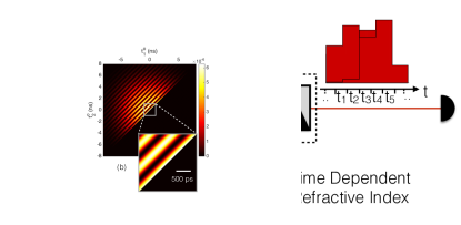
Figure 1: Schematic of (a) spatial mode Boson Sampling (SMBS) (b) temporal mode Boson Sampling (TMBS)

Figure 2: Schematic of TMBS with time-independent dispersion

SMBS entails several difficult challenges, that, as we show, favor temporal mode encoding. First, Boson Sampling requires an extremely large number of modes to be classically computationally difficult. Strictly speaking, the complexity argument for Boson Sampling assumes that, if $n$ is the number of photons in the system and $m$ is the number of modes, $m\geq\Omega(n^{5}\log^{2}n)$. Although Aaronson and Arkhipov have conjectured that the complexity arguments still hold when $m=O(n^{2})$ Aaronson and Arkhipov (2013), the number of modes is still large: e.g., even with $m=n^{2}$ and $n=30$, the interferometer would require 900 modes. Furthermore, the experiment would require 900 detectors and, if the photons came from heralded sources, 900 sources Lund et al. (2014). To date, experimental demonstrations of SMBS have been limited to 5 photons in 21 modes Carolan et al. (2014). The number of modes in temporal mode Boson Sampling (TMBS) can be increased simply by increasing the dispersion. Even with 10000 ps/nm dispersion, which can be achieved with off-the shelf components, and 100 ps detector jitter, which can be routinely achieved with silicon avalanche photodiodes or with superconducting nanowire single photon detectors Najafi et al. (2015), the number of modes in TMBS is orders of magnitude higher than SMBS. In principle, the experiment can be implemented in a single fiber with only a single photon source and only two detectors: one to herald input photons and one to detect the output state, regardless of the number of interfering photons in the system. Given the dead time $t_{dt}$ of single photon detectors, the output may have to be split between a larger number of detectors. However, in general, the number of detectors is smaller than required in SMBS .

Furthermore, uncertainty in the time when photons are injected into different modes leads to distinguishability and loss of boson interference. This is a particular problem in SMBS with heralded sources based on spontaneous parametric down conversion (SPDC). Most SMBS experiments to date have relied on downconverted photons. Temporal or spectral filtering could improve the interference, but at an exponential loss in multi-photon throughput. In TMBS, the lack of control over the input time of our photons only corresponds to a lack of control over the choice of our input modes; however, as long as the input modes are known, this does not affect the ability to perform Boson Sampling Lund et al. (2014).

Previous proposals have considered temporal modes for Boson Sampling Motes et al. (2014); Humphreys et al. (2013) but they relied on temporarily converting temporal modes to spatial modes and then mixing the modes with beamsplitter operations. Hence, increasing the number of output modes ($m\gg n$) requires a large number of effective beamsplitter operations. They also require active elements that operate on a picosecond time scale. Furthermore, since they are based on the interference of narrow photon packets, they suffer from the same issues with temporal mismatch as SMBS. In TMBS, detector jitter can limit the accuracy with which the input mode can be heralded but this limitation can be overcome by using large dispersion.

Time-independent dispersion - We first consider the simplest case of Boson Sampling in time with identically shaped input photons and time-independent dispersion (Fig. 2). If we use an SPDC source with idler photons heralded at times $t_{j}$ and signal photons used as input photons, the input state is given by $\ket{\Psi_{in}}=\left(\prod_{j}\hat{a}^{\dagger}_{Aj}\right)\ket{0}$ where $\ket{0}$ is the multimode vacuum state and $\hat{a}^{\dagger}_{Aj}\equiv\int_{-\infty}^{\infty}\textrm{d}t\ \hat{a}^{\dagger}(t)A(t-t_{j})$ represents the creation operator for the input state centered at $t_{j}$. $\hat{a}^{\dagger}(t)$ is the creation operator for time $t$ and $\omega_{0}$ is the central frequency of the input photons. We assume that the photon state after heralding of the idler is a pure state of the form $A(t-t_{j})$. However, a realistic detector projects the signal photon into a mixed state with $t_{j}$ varying over the timescale of the detector jitter; the effect of this temporal mismatch can be made negligible with large dispersion .

$\hat{a}^{\dagger}_{Aj}$ can be expanded in the frequency domain as $\hat{a}^{\dagger}_{Aj}=\int_{-\infty}^{\infty}\textrm{d}\omega\hat{a}^{\dagger}(\omega)\mathcal{F}\{A(t-t_{j})\}$ where $\hat{a}^{\dagger}(\omega)$ is the creation operator for frequency $\omega$ and $\mathcal{F}\{A(t-t_{j})\}$ is the Fourier transform of $A(t-t_{j})$. After passing through a dispersive element with dispersion relation $\beta(\omega)$ and length $L$, frequency components at $\omega$ are multiplied by a factor $\textrm{e}^{-i\phi(\omega)}$ where $\phi(\omega)\equiv\beta(\omega)L$. The wavefunction of the multi-photon system is then given by $\ket{\Psi_{out}}=\left(\prod_{j}\hat{b}^{\dagger}_{j}\right)\ket{0}$ where $\hat{b}^{\dagger}_{j}\equiv\int_{-\infty}^{\infty}\textrm{d}\omega\hat{a}^{\dagger}(\omega)\mathcal{F}\{A(t-t_{j})\}\textrm{e}^{-i\phi(\omega)}$. Going back to the time domain, $\hat{b}^{\dagger}_{j}=\int_{-\infty}^{\infty}\textrm{d}t\hat{a}^{\dagger}(t)U(t,t_{j})$ with

$$U(t,t_{j})=A(t-t_{j})*\mathcal{F}^{-1}\{\textrm{e}^{-i\phi(\omega)}\}$$ (1)

where ‘$*$’ is the convolution operator.

If dispersion parameters are chosen such that $U(t,t_{j})$ does not change appreciably when $t$ varies in a window of width $t_{s}$ , the modes can be discretized so that the transformation is well approximated by $\hat{a}^{\dagger}_{Aj}\rightarrow\sum_{i}U_{ij}\hat{a}^{\dagger}_{ti}$ where $\hat{a}^{\dagger}_{ti}$ represents the creation operator at the discretized time step near $t_{i}$, i.e. $\hat{a}^{\dagger}_{tj}=\int_{t_{j}}^{t_{j}+t_{s}}\textrm{d}t\hat{a}^{\dagger}(t)/\sqrt{t_{s}}$. We can then write the transformation as $\hat{a}^{\dagger}_{Aj}\rightarrow\sum_{i}U_{ij}\hat{a}^{\dagger}_{ti}=\int_{-\infty}^{\infty}\textrm{d}tU(t,t_{j})\hat{a}^{\dagger}(t_{i})$. If we assume that $U(t,t_{j})$ is approximately constant for a small time step $t_{s}$, we can approximate $U_{ij}\hat{a}^{\dagger}_{ti}\approx U(t_{i},t_{j})\int_{t_{j}}^{t_{j}+t_{s}}\textrm{d}t\hat{a}^{\dagger}(t)$. Hence, we have $U_{ij}=\sqrt{t_{s}}U(t_{i},t_{j})$. $\hat{a}^{\dagger}_{Aj}\rightarrow\sum_{i}U_{ij}\hat{a}^{\dagger}_{ti}$ where

$$U_{ij}=\left[\sqrt{t_{s}}A(t-t_{j})*\mathcal{F}^{-1}\{\textrm{e}^{-i\phi(\omega)}\}\right]_{t=t_{i}}$$ (2)

Eq. 2 shows the class of unitary transformations from which we can sample using time-independent dispersion. The unitary is band-diagonal because of the time-invariant nature of the system. Classical algorithms exist for the computation of the permanent of banded matrices with a banded inverse which is polynomial in the size of the matrix but exponential in the number of bands Temme and Wocjan (2012). The inverse of a unitary banded matrix is banded. However, because the number of bands is extremely large and the number of bands/dispersion is increased with the number of photons in order to limit the effect of jitter , the problem is still expected to be computationally hard.

The shape of the input pulses $A(t)$ is incorporated into the unitaries in Eq. 2 because, unlike conventional unitary implementations, the input states and measurement have different bases; the input photons have shape $A(t)$ but the measurement is in the time basis (with eigenfunctions $\delta(t-t_{j})$). The results of an experiment will be the same as a spatial unitary implementing Eq. 2. Imagine a fictitious experiment where the input photons are $\delta(t-t_{j})$. They then go through a unitary $U_{1}$ which puts them in a superposition of the form $A(t)$ (physically, this is the state of the photons going into the dispersion). The photons then go through another unitary $U_{2}$ which is the dispersion and the total unitary implemented by this system is $U_{1}U_{2}$. The output of this system will be the same as our scheme. Although a wavefunction $\delta(t-t_{j})$ is unphysical, the detector sees the same output state as if the operator $U_{1}U_{2}$ was applied to photons of the form $\delta(t-t_{j})$.

It is possible to sample from a larger class of unitaries by shaping the temporal form of the input photons. Methods for shaping single photons with arbitrary amplitude and phase in time have been proposed Kalachev (2010) and an experimental demonstration of shaping the spatial waveform of single photons had been reported Köprülü et al. (2011). With pulse-shaping, the input waveform $A(t-t_{j})$ is replaced by a more general set of functions $A_{j}(t)$ so that the accessible set of unitaries becomes

$$U_{ij}=\left[\sqrt{t_{s}}A_{j}(t)*\mathcal{F}^{-1}\{\textrm{e}^{-i\phi(\omega)}\}\right]_{t=t_{i}}$$ (3)

If it were possible to choose any set of functions $A_{j}(t)$, then the unitary could be chosen column by column using $A_{j}$ and simply detecting the photons without any dispersion would be equivalent to Boson Sampling. However, it is experimentally challenging to prepare multiple overlapping photons with a specific waveform. Hence, for realistic implementation, the photon wave-packets should be separated in time. This limits the possible unitaries represented by Eq. 3.

Although we have no proof of the hardness of sampling from such a unitary, there is to our knowledge no reported efficient classical algorithm for sampling from a general unitary of this form. Sending a train of photons through a time-independent dispersion could allow for a Boson Sampling experiment with more photons and more modes than can be currently achieved with SMBC.

An arbitrary functional form for the dispersion $\phi(\omega)$ can be obtained by using approaches used in optical functional design Madsen and Zhao (1999) and femtosecond pulse-shaping Weiner (2000). There are even commercial products for implementing arbitrary dispersion used for pulse-shaping in telecommunication .

A central feature in spatial boson collision experiments is the bunching of bosons in the output modes i.e., Hong-Ou-Mandel interference Hong et al. (1987). An analogous feature appears in the temporal modes. Consider a heralded input state of two photons, $a^{\dagger}(t-t_{1}^{i})a^{\dagger}(t-t_{2}^{i})\ket{0}$. If this state passes through group velocity dispersion in a fiber of length $L$: $\beta(\omega)=\beta_{0}+\beta_{1}(\omega-\omega_{0})+1/2\beta_{2}(\omega-\omega_{0})^{2}$, $\phi_{j}=\beta_{j}L,j\in\{0,1,2\}$. For simplicity, we have assumed a Gaussian input shape of the form

$$A(t)=\left(\frac{1}{\sigma_{cor}\sqrt{2\pi}}\right)^{1/2}\exp{\left[-\frac{t^{2}}{4\sigma_{cor}^{2}}\right]}\exp[i\omega_{0}t],$$ (4)

where we have assumed that the correlation time $\sigma_{cor}$ of the photons from the heralded photon source is much shorter than the biphoton coherence time. SPDC photons are often approximated as Gaussians in time. However, the two photon interference effects would be visible with any shape in general. After passing through this dispersive element, the probability of detecting the photons at times $t^{o}_{1}$ and $t^{o}_{2}$ corresponds to the magnitude squared of a $2\times 2$ permanent and assuming $\phi_{2}\gg\sigma_{cor}^{2}$, the probability goes to zero when

$$\Delta t^{i}\Delta t^{o}=(2m+1)\pi\phi_{2}$$ (5)

Figure 3: (a) Setup for seeing ’HOM-like’ interference (b) The joint probability of detecting the first photon at $t^{o}_{1}$ and the second photon at $t^{o}_{2}$ when two input photons near t = 0 and separated by 100 ps are sent through a second order dispersive element. $\sigma_{cor}$ = 200 fs and the dispersive element has a GVD parameter of magnitude $|D|$ = $2\pi c\phi_{2}/\lambda^{2}$ = 10000 ps/nm. $t_{s}=10$ ps

In Fig. 3, the joint probability of observing a photon at $t^{o}_{1}$ and $t^{o}_{2}$ is plotted when two photons with $\sigma_{cor}$ = 200 fs and a Gaussian temporal waveform centered at $t^{i}_{1}=-\phi_{1}$ and $t^{i}_{2}=-\phi_{1}+100$ ps are sent through a dispersive element with a GVD parameter of magnitude $|D|$ = $2\pi c\phi_{2}/\lambda^{2}$ = 10000 ps/nm. The assumption $\phi_{2}\gg\sigma_{cor}^{2}$ has not been used. At the time-scale of a few nanoseconds, the output resembles a Gaussian pulse centered at $t^{o}=0$, as would be expected from single photon input at $t^{i}=-\phi_{1}$. However, at the time scale of hundreds of picoseconds, two-photon interference effects can be seen in clear dips in the two-photon output probability appear, as predicted by Eq. 5. The plot has been discretized with $t_{s}=10$ ps. We chose a low value of $t_{s}$ here to clearly show the shape of our interference pattern; such timing resolution is not necessarily required to resolve the two-photon interference pattern. Experimentally, these dips would be easily resolved using detectors with a jitter of 100 ps. The predicted correlation measurement is provided in Fig. 1 of the supplemental material . The increase in the size of each bin would also increase the probability of detecting photons in each time bin by a factor of 100.

Figure 4: Schematic of TMBS with time-dependent dispersion

Time-dependent dispersion - With time-dependent dispersion, it is possible to implement any arbitrary unitary transformation on temporal modes.

Using the time projection operator $\hat{t}_{p}=\int\textrm{d}t^{\prime}\ t\ket{t^{\prime}}\bra{t^{\prime}}$ and the frequency projection operator $\hat{\omega}_{p}=\int\textrm{d}\omega\ \omega\ket{\omega}\bra{\omega}$ which satisfy $[\hat{t}_{p},\hat{\omega}_{p}]=i/2$ (similar to $\hat{x}$ and $\hat{p}$ in Lloyd and Braunstein (1999); Sefi and van Loock (2011)), an arbitrary continuous variable unitary on temporal modes can be written as $\textrm{e}^{-if(\hat{t}_{p},\hat{\omega}_{p})}$ where $f(\hat{t}_{p},\hat{\omega}_{p})=\int\textrm{d}tH(\hat{t}_{p},\hat{\omega}_{p},t)$. $H(\hat{t}_{p},\hat{\omega}_{p},t)$ is the Hamiltonian of the system. It should be noted that $\hat{t}_{p}$ is the time projection operator corresponding to the photon’s temporal waveform and not the time over which the system evolves. Hence, the variable of integration $t$ above is distinct from the operator $\hat{t}_{p}$ .

Such a Hamiltonian can be physically realized by making the elements of the dispersion time-dependent. In the previous section we discussed methods for implementing arbitrary dispersion which implements a Hamiltonian of the form $\phi(\hat{\omega}_{p})$. Since photons reaching the dispersive element at different times see a different $\phi(\hat{\omega}_{p})$, the Hamiltonian can be written as $H(\hat{t}_{p},\hat{\omega}_{p},t)$ where $H$ can be any real function. Hence, we get the desired unitary $\textrm{e}^{-if(\hat{t}_{p},\hat{\omega}_{p})}$ with time-dependent elements that allow for changes in the frequency spectrum of the pulses which was not possible with time-independent dispersion.

Another option for realizing such a unitary would be to cascade elements that implement time-independent dispersion and a time-dependent refractive index. The Hamiltonians corresponding to dispersion and time dependent refractive index are $\phi(\hat{\omega}_{p})$ and $g(\hat{t}_{p})$ respectively.

Following previous work on realizing arbitrary Hamiltonians for continuous variable systems Lloyd and Braunstein (1999); Sefi and van Loock (2011), one can construct Hamiltonians of the form $[g_{1}(\hat{t}_{p}),\phi_{1}(\hat{\omega}_{p})]+[g_{2}(\hat{t}_{p}),[g_{3}(\hat{t}_{p}),\phi_{3}(\hat{\omega}_{p})]]+.....$ using the properties

$$\textrm{e}^{-i\hat{A}\delta t}\textrm{e}^{-i\hat{B}\delta t}\textrm{e}^{i\hat{A}\delta t}\textrm{e}^{i\hat{B}\delta t} = \textrm{e}^{[\hat{A},\hat{B}]\delta t^{2}}+O(\delta t^{3})$$ (6)

$$\textrm{e}^{i\hat{A}\delta t/2}\textrm{e}^{i\hat{B}\delta t/2}\textrm{e}^{i\hat{B}\delta t/2}\textrm{e}^{i\hat{A}\delta t/2} = \textrm{e}^{i(\hat{A}+\hat{B})\delta t}+O(\delta t^{3}).$$ (7)

The following Hamiltonians can be cascaded to generate a Hamiltonian that can be any polynomial in $\hat{t}_{p}$ and $\hat{\omega}_{p}$ Lloyd and Braunstein (1999): $\hat{t}_{p}$, $\hat{\omega}_{p}$, $\hat{t}_{p}^{2}+\hat{\omega}_{p}^{2}$ and a Hamiltonian of the form $\hat{\omega}_{p}^{n}$ where $n\geq 3$. The Hamiltonians $\hat{\omega}_{p}$ and $\hat{t}_{p}$ are first order dispersion (inverse group velocity) and a linear varying refractive index. A high order Hamiltonian $\hat{\omega}_{p}^{n}$ can be realized with higher order dispersion. $\hat{t}_{p}^{2}+\hat{\omega}_{p}^{2}$ can be realized with a combination of second order dispersion and a quadratically varying refractive index using Eq. 7. Although such a decomposition allows us to build arbitrary Hamiltonians with a number of elements which increase as a small polynomial in the number of photons Braunstein (2005), more efficient decompositions are often possible with fewer elements Sefi and van Loock (2011).

Furthermore, as opposed to the conventional construction of $f(\hat{x},\hat{p})$ Lloyd and Braunstein (1999) which uses low-order polynomials in $\hat{x}$ and $\hat{p}$ (high order polynomials require a non-linear medium), a unitary of the form $g(\hat{t}_{p})$ or $\phi(\hat{\omega}_{p})$ can be of any arbitrary functional form without requiring an explicit Kerr-type nonlinearity.

Given the ability to realize arbitrary continuous variable single particle unitaries over $\hat{t}_{p}$, any discrete unitary transformation can be implemented by making the transformation constant over the output time bins . Such an experiment with multiple photons would be equivalent to Boson Sampling and if the discrete unitary is chosen with Haar measure, the results are believed to be classically intractable Aaronson and Arkhipov (2013).

In conclusion, we have introduced new methods of implementing unitary transformations on temporal modes based on dispersion and pulse shaping that require a much smaller number of sources and detectors and do not require a large system of beamsplitters. In principle, using only fixed dispersion, a single heralded source and two detectors, one can observe multi-photon interference and perform a Boson Sampling experiment for which no efficient classical algorithm is known, to our knowledge. By using time-dependent dispersion, it is possible to sample from arbitrary unitaries.

We would like to thank Scott Aaronson, Alex Arkhipox, Gian Guerreschi and Ish Dhand for helpful discussions. This work was supported by the AFOSR MURI program under grant number (FA9550-14-1-0052).

We welcome any suggestions on this paper. You may contact us directly or submit comments at http://goo.gl/forms/4YA8xRBj9s (you may submit comments anonymously).

References

- Kok et al. (2007) P. Kok, K. Nemoto, T. C. Ralph, J. P. Dowling, and G. J. Milburn, Reviews of Modern Physics 79, 135 (2007).
- O’Brien et al. (2009) J. L. O’Brien, A. Furusawa, and J. Vučković, Nature Photonics 3, 687 (2009).
- Peruzzo et al. (2010) A. Peruzzo, M. Lobino, J. C. F. Matthews, N. Matsuda, A. Politi, K. Poulios, X.-Q. Zhou, Y. Lahini, N. Ismail, K. Wörhoff, Y. Bromberg, Y. Silberberg, M. G. Thompson, and J. L. OBrien, Science (New York, N.Y.) 329, 1500 (2010).
- Aaronson and Arkhipov (2013) S. Aaronson and A. Arkhipov, Theory of Computing 9, 143 (2013).
- Spring et al. (2013) J. B. Spring, B. J. Metcalf, P. C. Humphreys, W. S. Kolthammer, X.-M. Jin, M. Barbieri, A. Datta, N. Thomas-Peter, N. K. Langford, D. Kundys, J. C. Gates, B. J. Smith, P. G. R. Smith, and I. A. Walmsley, Science (New York, N.Y.) 339, 798 (2013).
- Broome et al. (2013) M. A. Broome, A. Fedrizzi, S. Rahimi-Keshari, J. Dove, S. Aaronson, T. C. Ralph, and A. G. White, Science (New York, N.Y.) 339, 794 (2013).
- Tillmann et al. (2013) M. Tillmann, B. Dakić, R. Heilmann, S. Nolte, A. Szameit, and P. Walther, Nature Photonics 7, 540 (2013).
- Crespi et al. (2013) A. Crespi, R. Osellame, R. Ramponi, D. J. Brod, E. F. Galvão, N. Spagnolo, C. Vitelli, E. Maiorino, P. Mataloni, and F. Sciarrino, Nature Photonics 7, 545 (2013).
- Carolan et al. (2014) J. Carolan, J. D. A. Meinecke, P. J. Shadbolt, N. J. Russell, N. Ismail, K. Wörhoff, T. Rudolph, M. G. Thompson, J. L. O’Brien, J. C. F. Matthews, and A. Laing, Nature Photonics 8, 621 (2014).
- Tillmann et al. (2014) M. Tillmann, S.-H. Tan, S. E. Stoeckl, B. C. Sanders, H. de Guise, R. Heilmann, S. Nolte, A. Szameit, and P. Walther, (2014), arXiv:1403.3433 .
- Spagnolo et al. (2014) N. Spagnolo, C. Vitelli, M. Bentivegna, D. J. Brod, A. Crespi, F. Flamini, S. Giacomini, G. Milani, R. Ramponi, P. Mataloni, R. Osellame, E. F. Galvão, and F. Sciarrino, Nature Photonics 8, 615 (2014), arXiv:1311.1622 .
- Turchette et al. (1995) Q. Turchette, C. Hood, W. Lange, H. Mabuchi, and H. Kimble, Physical Review Letters 75, 4710 (1995).
- Knill et al. (2001) E. Knill, R. Laflamme, and G. J. Milburn, Nature 409, 46 (2001).
- Lund et al. (2014) A. P. Lund, A. Laing, S. Rahimi-Keshari, T. Rudolph, J. L. O’Brien, and T. C. Ralph, Physical Review Letters 113, 100502 (2014).
- Najafi et al. (2015) F. Najafi, J. Mower, N. C. Harris, F. Bellei, A. Dane, C. Lee, X. Hu, P. Kharel, F. Marsili, S. Assefa, K. K. Berggren, and D. Englund, Nature Communications 6, 5873 (2015).
- Note (1) See Supplemental Material.
- Motes et al. (2014) K. R. Motes, A. Gilchrist, J. P. Dowling, and P. P. Rohde, , 7 (2014), arXiv:1403.4007 .
- Humphreys et al. (2013) P. C. Humphreys, B. J. Metcalf, J. B. Spring, M. Moore, X.-M. Jin, M. Barbieri, W. S. Kolthammer, and I. A. Walmsley, Physical Review Letters 111, 150501 (2013).
- Temme and Wocjan (2012) K. Temme and P. Wocjan, (2012), arXiv:1208.6589 .
- Kalachev (2010) A. Kalachev, Physical Review A 81, 043809 (2010).
- Köprülü et al. (2011) K. G. Köprülü, Y.-P. Huang, G. A. Barbosa, and P. Kumar, Optics letters 36, 1674 (2011).
- Madsen and Zhao (1999) C. K. Madsen and J. H. Zhao, Optical Filter Design and Analysis: A Signal Processing Approach, edited by K. Chang (Wiley Online Library, 1999).
- Weiner (2000) A. M. Weiner, Review of Scientific Instruments 71, 1929 (2000).
- Note (2) See https://www.finisar.com/optical-instrumentation.
- Hong et al. (1987) C. K. Hong, Z. Y. Ou, and L. Mandel, Physical Review Letters 59, 2044 (1987).
- Lloyd and Braunstein (1999) S. Lloyd and S. Braunstein, Physical Review Letters 82, 1784 (1999).
- Sefi and van Loock (2011) S. Sefi and P. van Loock, Physical Review Letters 107, 170501 (2011).
- Braunstein (2005) S. L. Braunstein, Reviews of Modern Physics 77, 513 (2005).