The generalized Chaplygin–Jacobi gas

Abstract

The present paper is devoted to find a new generalization of the generalized Chaplygin gas. Therefore, starting from the Hubble parameter associated to the Chaplygin scalar field and using some elliptic identities, the elliptic generalization is straightforward. Thus, all relevant quantities that drive inflation are calculated exactly. Finally, using the measurement on inflation from the Planck 2015 results, observational constraints on the parameters are given.

1 Introduction

Clearly, evidence from the most varied observations suggest that near 25% of the cosmic energy–matter corresponds to the so-called cold dark matter (CDM) and the remaining 75% corresponds to the so-called dark energy (DE). The dark matter problem born with the Zwicky’s observation of a large velocity dispersion of the components in the Coma cluster [1] together with Babcock observation of galactic rotation curves in the Andromeda galaxy [2]. This paradigm has been studied in several context, for example from the particle physics point of view, the candidates are axions, inert Higgs doublet, sterile neutrinos, super–symmetric particles and Kaluza–Klein particles [3, 4, 5, 6, 7], while from the geometrical point of view Weyl’s theory has received much attention from theoretical and experimental physicists [8, 9, 10, 11, 12, 13, 14, 15]. On the other hand, one of the most natural candidates to explain DE corresponds to a cosmological constant $\Lambda$, which, although successful as a fit model, it shows a huge discrepancy between its theoretical and observed values [16]. This evidence has promoted the study of new types of candidates that can link the different stage of the universe. One type of cosmic fluid is often called quintessence and has been widely used because it behaves like a cosmological constant by combining positive energy density and negative pressure. Nevertheless, unlike the cosmological constant, the pressure of this fluid is dynamic. An example of this type is the so-called Chaplygin gas (CG) which is an exotic fluid having the equation of state (EoS)

$$p_{ch}=-\frac{B}{\rho_{ch}},$$ (1.1)

where $B$ is a positive constant, $p_{ch}$ and $\rho_{ch}$ are the pressure and energy density in a comoving reference frame, respectively. This EoS was originally proposed to describe the lifting force on a wing of an airplane in aerodynamics [17]. In cosmology, it was first introduce by [18, 19, 20], nevertheless, in its original form, this fluid presents inconsistency with some observational data [21, 22, 23] such that a generalization is necessary to improve consistency with data. A first attempt was made considering the generalized Chaplygin gas (GCG) whose EoS is given by [24, 25, 26, 27]

$$p_{gcg}=-\frac{B}{\rho_{gcg}^{\alpha}},$$ (1.2)

where $B>0$ and the GCG parameter lies in the range $0\leq\alpha\leq 1$. Obviously, the CG is recovered by making $\alpha=1$, while the case $\alpha=0$ mimics the effect of a cosmological constant. An important characteristic of the Chaplygin gas (CG and GCG) is that this interpolates between a dust dominated phase where $\rho\propto a^{-3}$, and a de Sitter phase where $p=-\rho$. The different parameters that enter into the model has been confronted successfully with many observational data (see, for example [28, 29, 30]), but, unfortunately, the model produce oscillations or exponential blowup in the matter power spectrum, being inconsistent with observation [31].

On the other hand, an approach to single-field inflation using the GCG as inflaton field was performed by del Campo [32]. By comparing with the measurement for the scalar spectral index together with its running from the Planck 2013 data [34], del Campo found that the best value for the $\alpha$–parameter is given by $\alpha=0.2578\pm 0.0009$. Therefore, following the idea outlined in [35], the main goal of this paper is to give a new generalization for the Chaplygin scalar field by using elliptic functions to describe the inflationary stage and then perform the confrontation between the model and the measurement recently released by the Planck 2015 data.

The outline of this work is as follows: the basic aspects to describe exact solutions to inflationary universe models within the framework of the Hamilton–Jacobi approach to cosmology, together with review of the results found earlier by del Campo for the GCG are showed in Section II. In Section III the Chaplygin–Jacobi gas is presented and the Hamilton–Jacobi formalism is applied to find the most relevant quantities in the inflationary stage. Finally, in Section IV conclusions and final remarks are presented. In addition, Appendix A few useful formulas and identities that satisfy the Jacobi elliptic functions are shown.

2 The generalized Chaplygin gas in inflation

The fundamental quantity in inflation is the scalar inflaton field $\phi$ which leads to the universe to expand extremely rapid in a very short time. The evolution of this field becomes governed by its scalar potential, $V(\phi)$, via the Klein–Gordon equation

$$\ddot{\phi}+3H\dot{\phi}+V_{,\phi}=0,$$ (2.1)

where $V_{,\phi}$ represents a derivative with respect to $\phi$. Thus, this equation of motion, together with the Friedmann equation,

$$H^{2}=\frac{8\pi}{3m_{p}^{2}}\left[\frac{1}{2}\dot{\phi}^{2}+V(\phi)\right]$$ (2.2)

obtained from Einstein general relativity theory, form the most simple set of field equations, which could be applied to obtain inflationary solutions. The set of equations (2.1-2.2) are the mainstay of Hamilton–Jacobi approach [36, 37, 38, 39, 40, 41, 42].

In order to obtain exact solutions in this approach, del Campo [32] and Dinda et al [33] used the Chaplygin gas whose generating function is given by

$$H(\phi)=H_{0}\cosh^{\frac{1}{1+\alpha}}\left[(1+\alpha)\Phi)\right],$$ (2.3)

where $\Phi\equiv\sqrt{\frac{6\pi}{m_{p}^{2}}}(\phi-\phi_{0})$ is a dimensionless scalar field and $H_{0}$, the value of $H$ when $\phi=\phi_{0}$, is a constant given by $H_{0}=\sqrt{\frac{8\pi}{3m_{p}^{2}}}\,B^{\frac{1}{2(1+\alpha)}}$. From the generating function (2.3) one can obtain all the relevant quantities for inflation, for example the scale factor

$$a(\phi)=a_{i}\,\exp\left[-\frac{4\pi}{m_{p}^{2}}\,\int_{\phi_{i}}^{\phi}\frac{H(\phi)}{H_{,\phi}(\phi)}d\phi\right],$$ (2.4)

which becomes

$$a(\phi)=a_{i}\,\left(\frac{\sinh[(1+\alpha)\Phi]}{\sinh[(1+\alpha)\Phi_{i}]}\right)^{\frac{2}{3(1+\alpha)}}.$$ (2.5)

The number of e-folding of physical expansion that occur in the inflationary stage is given by

$$N\equiv\int_{t_{i}}^{t_{f}}H\,dt=\frac{4\pi}{m_{p}^{2}}\int_{\phi_{f}}^{\phi_{i}}\frac{H}{H_{,\phi}}\,d\phi,$$ (2.6)

so, del Campo found that for the GCG this quantity becomes

$$N(\phi)=\frac{2}{3(1+\alpha)}\,\mathrm{ln}\left\{\frac{\sinh[(1+\alpha)\Phi_{e}]}{\sinh[(1+\alpha)\Phi]}\right\},$$ (2.7)

while the scalar potential

$$V(\phi)=\left(\frac{3m_{p}^{2}}{8\pi}\right)\left[H^{2}-\frac{m_{p}^{2}}{12\pi}H_{,\phi}^{2}\right],$$ (2.8)

is given by the following expression:

$$V(\phi)=V_{0}\,\frac{1+\cosh^{2}[(1+\alpha)\Phi]}{\cosh^{\frac{2\alpha}{1+\alpha}}[(1+\alpha)\Phi]},$$ (2.9)

where $V_{0}=\frac{1}{2}B^{\frac{1}{1+\alpha}}$. In the slow–rolls approximation this scalar potential is well behaved and reduces to

$$V_{s-r}(\phi)\simeq V_{0}\cosh^{\frac{2}{1+\alpha}}[(1+\alpha)\Phi].$$ (2.10)

In next section, the Hamilton–Jacobi formalism is applied to obtain exact solutions in the inflationary stage using a elliptic generalization of the GCG.

3 The generalized Chaplygin–Jacobi gas

It is well known that trigonometric and hyperbolic functions are special cases of more general functions, the so-called elliptic functions, which are doubly periodic in the complex plane, while the above are periodic on the real axis and the imaginary axis, respectively. With this in mind and using the rules given in appendix A, the generating function (2.3) is conveniently written as

$$H(\phi,k)=H_{0}\,\textrm{nc}^{\frac{1}{1+\alpha}}\left[(1+\alpha)\,\Phi\right],$$ (3.1)

where $\textrm{nc}(x)=1/\textrm{cn}(x)$, and $\textrm{cn}(x)\equiv\textrm{cn}(x|\,k)$ is the Jacobi elliptic cosine function, and $k$ is the modulus. This choice allows to obtain the generating function of the GCG (2.3) making $k\rightarrow 1$ in equation (3.1). Henceforth we denote this scalar field as the generalized Chaplygin–Jacobi gas (GCJG).

Taking into account that pressure and energy density are given by

$$p_{\phi}=\frac{3m_{p}^{2}}{8\pi}H^{2}\left[\frac{m_{p}^{2}}{6\pi}\left(\frac{H_{,\phi}}{H}\right)^{2}-1\right]$$ (3.2)

and

$$\rho_{\phi}=\frac{3m_{p}^{2}}{8\pi}H^{2},$$ (3.3)

respectively, and by using the generating function (3.1) it is no hard to obtain that

$$p_{\phi}=-\frac{B^{\frac{1}{2(1+\alpha)}}}{k}\,\text{nc}^{\frac{2(2+\alpha)}{1+\alpha}}\left[(1+\alpha)\,\Phi\right]\,(\text{dn}^{4}\left[(1+\alpha)\,\Phi\right]-k^{\prime}),$$ (3.4)

and

$$\rho_{\phi}=B^{\frac{1}{2(1+\alpha)}}\,\textrm{nc}^{\frac{2}{1+\alpha}}\left[(1+\alpha)\,\Phi\right],$$ (3.5)

where $k^{\prime}=1-k$ is the complementary modulus. Therefore, by using eq. (3.5) one obtain $\textrm{nc}\left[(1+\alpha)\,\Phi\right]$ as a function of $\rho_{\phi}$ and then, by substituting into eq. (3.4) together with some identities of the Jacobi elliptic functions, the EoS related to the GCJG read

$$p_{\phi}=-\frac{B\,k}{\rho_{\phi}^{\alpha}}-2\,k^{\prime}\,\rho_{\phi}+\frac{k^{\prime}}{B}\,\rho_{\phi}^{2+\alpha}$$ (3.6)

Obviously, in the limit $k\rightarrow 1$ (or $k^{\prime}\rightarrow 0$) this EoS coincide with (1.2).

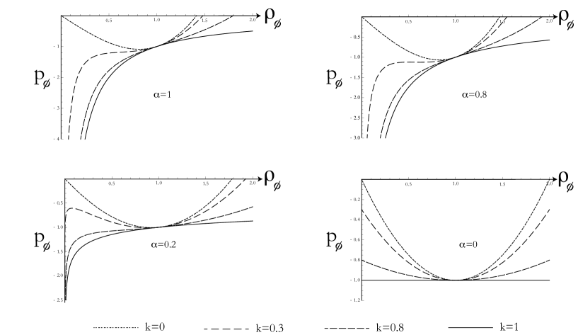
Figure 1: Plot of the pressure against density for generalized Chaplygin–Jacobi gas (3.6). Here we plot different values of the modulus $k$ and GCG parameter $\alpha$. In all graphs was used $B=1$.

Note that, for $k\neq 1$, the GCJG presents a novel behaviour in which the pressure is a positive quantity. This fact occurs at the range $\rho_{\phi}^{(c)}<\rho_{\phi}$, where critical density, $\rho_{\phi}^{(c)}$, depends on the parameters across the following expression

$$\rho_{\phi}^{(c)}=\left[B\left(1+\frac{1}{\sqrt{k^{\prime}}}\right)\right]^{\frac{1}{1+\alpha}}.$$ (3.7)

At this point $p_{\phi}=0$, and the fluid presents a dust–like behaviour. An interesting feature of this EoS appears when $k=0$ (or $k^{\prime}=1$) which corresponds to the trigonometric limit. In addition to the root obtained from equation (3.7), must also add $\rho_{\phi}^{(c)}=0$, and therefore the GCJG presents a dust–like behaviour when $\rho_{\phi}=0$ and $\rho_{\phi}=(2\,B)^{\frac{1}{1+\alpha}}$, as shown in Figure 1.

For this fluid one has simply that the EoS parameter becomes

$$\omega_{\phi}=\frac{p_{\phi}}{\rho_{\phi}}=\frac{k^{\prime}}{B}\rho_{\phi}^{1+\alpha}-\frac{B\,k}{\rho_{\phi}^{1+\alpha}}-2\,k^{\prime},$$ (3.8)

while the square of the speed of sound is

$$v_{\phi}^{2}=\frac{\partial p_{\phi}}{\partial\rho_{\phi}}=\frac{(2+\alpha)\,k^{\prime}}{B}\rho_{\phi}^{1+\alpha}+\frac{B\,k\,\alpha}{\rho_{\phi}^{1+\alpha}}-2\,k^{\prime}.$$ (3.9)

Note that the speed of sound vanished when the density reaches the value

$$\rho_{\phi}^{(0)}=\left[B\left(\frac{1\pm\sqrt{1-\frac{k}{k^{\prime}}\alpha(2+\alpha)}}{2+\alpha}\right)\right]^{\frac{1}{1+\alpha}}.$$ (3.10)

Of course, the existence of these points is restricted to pairs that satisfy the condition $k^{-1}>(1+\alpha)^{2}$. For example, if $\alpha=0$, then $k<1$, while for the case $\alpha=1$ the modulus must be $k<0.25$. It is important to note that null speed of sound do not implies null pressure. In fact, at this point the pressure is

$$p_{\phi 0}\equiv p_{\phi}(\rho_{\phi}=\rho_{\phi}^{(0)})=\frac{2B(1+\alpha)}{(2+\alpha)^{2}\,(\rho_{\phi}^{(0)})^{\alpha}}\left\{1+k(1+\alpha)\pm\sqrt{k^{\prime}\,[1-k(1+\alpha)^{2}]}\right\}.$$ (3.11)

On the other hand, using eq. (2.8) together with eq. (3.1) one obtain for the scalar potential

$$V(\phi)=V_{0}\frac{2\text{nc}^{2}\left[(1+\alpha)\,\Phi\right]-\text{dc}^{2}\left[(1+\alpha)\,\Phi\right]\,\text{sc}^{2}\left[(1+\alpha)\,\Phi\right]}{\textrm{nc}^{\frac{2\alpha}{1+\alpha}}\left[(1+\alpha)\,\Phi\right]},$$ (3.12)

where $V_{0}=\frac{1}{2}B^{\frac{1}{2(1+\alpha)}}$. This scalar potential is depicted in Figure 2 for different values of the GCG parameter $\alpha$ and the modulus $k$.

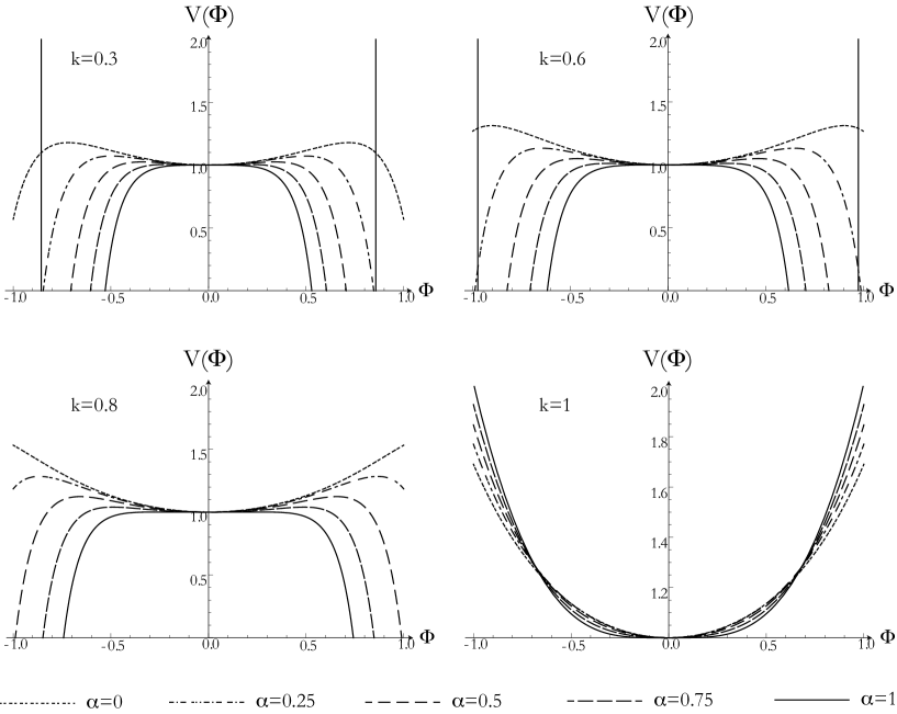
Figure 2: Plots of the scalar potentials for generalized Chaplygin–Jacobi gas, $V(\Phi)$, as a function of the dimensionless scalar field, $\Phi\equiv\sqrt{\frac{6\pi}{m_{p}^{2}}(\phi-\phi_{0})}$. Here the scalar potential $V(\Phi)$ is expressed as a multiple of the constant $V_{0}\equiv\frac{1}{2}B^{\frac{1}{1+\alpha}}$.

Also, by using eqs. (2.8) and (3.1) is straightforward to found the potential as a function of the generating function, so

$$V(H)=V_{0}\left(\frac{H}{H_{0}}\right)^{2}\left\{2-\left[k^{\prime}\left(\frac{H}{H_{0}}\right)^{2(1+\alpha)}+k\right]\left[1-\left(\frac{H_{0}}{H}\right)^{2(1+\alpha)}\right]\right\}.$$ (3.13)

By combining the generating function (3.1) with eq. (2.4) allows to find the scale factor as a function of the inflaton field:

$$a(\phi)=a_{i}\,\left(\frac{\textrm{sd}[(1+\alpha)\Phi]}{\textrm{sd}[(1+\alpha)\Phi_{i}]}\right)^{\frac{2}{3(1+\alpha)}}.$$ (3.14)

Here $\textrm{sd}(x)\equiv\textrm{sd}(x|\,k)=\textrm{sn}(x)/\textrm{dn}(x)$, where $\textrm{sn}(x)\equiv\textrm{sn}(x|\,k)$ is the Jacobi elliptic sine function and $\textrm{dn}(x)\equiv\textrm{dn}(x|\,k)$ is the Jacobi elliptic delta function.

With the aim to verify that an inflationary period occurs, it is very helpful to introduce the deceleration parameter $q=\frac{m_{p}^{2}}{4\pi}\left(\frac{H_{,\phi}}{H}\right)^{2}-1$, which becomes

$$q=\frac{3}{2}\frac{\text{dn}^{2}\left[(1+\alpha)\,\Phi\right]\,\text{sn}^{2}\left[(1+\alpha)\,\Phi\right]}{\text{cn}^{2}\left[(1+\alpha)\,\Phi\right]}-1.$$ (3.15)

Making use of some elliptic identities it is possible obtain the value for $\phi_{e}$, the value for the scalar field when inflation ends (i. e. $q(\phi_{e})=0$). For example, if eq. (3.15) is writes in terms of the Jacobi elliptic sine one arrives to the following quadratic equation

$$3k\,y^{2}-5\,y+2=0,$$ (3.16)

where $y=\text{sn}^{2}\left[(1+\alpha)\,\Phi_{e}\right]$. Therefore, solving for $\Phi_{e}$ one get that the four roots are given by

$$\Phi_{e}=\frac{F\left[\arcsin\left(\pm\sqrt{y_{\pm}}\right),\,k\right]}{1+\alpha},$$ (3.17)

where $F(\varphi,\,k)$ is the normal elliptic integral of the first kind and

$$y_{\pm}=\frac{5}{6k}\left(1\pm\sqrt{1-\frac{24\,k}{25}}\right).$$ (3.18)

It is important to note that real solutions are found for all $0\leq k\leq 1$. Also, the condition $y\leq 1$ implies that the allowed solution are $\pm\sqrt{y_{-}}$.

On the other hand, using eq. (2.6) one get that the number of the e-folds becomes

$$N(\phi)=\frac{2}{3(1+\alpha)}\ln\left\{\frac{\textrm{sd}[(1+\alpha)\Phi_{e}]}{\textrm{sd}[(1+\alpha)\Phi]}\right\},$$ (3.19)

where $\Phi_{e}$ is given by eq. (3.17). For example, for $N=70$ the above leads to

$$\Phi_{70}=\frac{F\left[\arcsin\left(\frac{x}{\sqrt{1+kx^{2}}}\right),\,k\right]}{1+\alpha},$$ (3.20)

where $x$ is given by

$$x=\textrm{sd}[(1+\alpha)\Phi_{e}]\,e^{-105(1+\alpha)}.$$ (3.21)

In order to obtain some information about the perturbations, result instructive to define the three first hierarchy parameters in terms of the generating function and its derivatives. Thus, the first Hubble hierarchy parameter $\epsilon_{H}$ is given by

$$\epsilon_{H}\equiv-\frac{d\ln H}{d\ln a}=\left(\frac{m_{p}^{2}}{4\pi}\right)\left(\frac{H_{,\phi}}{H}\right)^{2}.$$ (3.22)

Note that this parameter provides information about the acceleration of the universe, so during inflation the bound $\epsilon_{H}\ll 1$ is fulfilled, and inflation ends once $\epsilon_{H}=1$. Taking account that $\epsilon_{H}=q+1$, one obtain from (3.15) that

$$\epsilon_{H}=\frac{3}{2}\frac{\text{dn}^{2}\left[(1+\alpha)\,\Phi\right]\,\text{sn}^{2}\left[(1+\alpha)\,\Phi\right]}{\text{cn}^{2}\left[(1+\alpha)\,\Phi\right]}.$$ (3.23)

The second Hubble hierarchy $\eta_{H}$ is defined as

$$\eta_{H}\equiv-\frac{d\,\ln H_{,\phi}}{d\,\ln a}=\left(\frac{m_{p}^{2}}{4\pi}\right)\left(\frac{H_{,\phi\phi}}{H}\right),$$ (3.24)

where plugging the Chaplygin–Jacobi scalar field becomes

$$\eta_{H}=\epsilon_{H}\left\{\frac{1+\alpha\,\textrm{cn}^{2}[(1+\alpha)\Phi]}{\textrm{sn}^{2}[(1+\alpha)\Phi]}+\frac{(1+\alpha)\,k^{\prime}}{\textrm{dn}^{2}[(1+\alpha)\Phi]}\right\}.$$ (3.25)

Finally, the third Hubble hierarchy parameter, $\xi_{H}^{2}$ is defined by

$$\xi_{H}^{2}\equiv\left(\frac{m_{p}^{2}}{4\pi}\right)^{2}\,\left(\frac{H_{,\phi}\,H_{,\phi\phi\phi}}{H^{2}}\right),$$ (3.26)

which becomes

$$\xi_{H}^{2}=\epsilon_{H}^{2}\left\{\frac{(2\alpha^{2}+7\alpha+6)\,k^{\prime}}{\textrm{sn}^{2}\,[(1+\alpha)\Phi]\,\textrm{dn}^{2}\,[(1+\alpha)\Phi]}+\frac{3}{2\epsilon_{H}}\left[(2k-1)-k\,\alpha\,(1+2\alpha)\,\textrm{cn}^{2}\,[(1+\alpha)\Phi]\right]\right\}.$$ (3.27)

The quantum fluctuations produce a power spectrum of scalar density fluctuations of the form [43, 44]

$$\mathcal{P}_{\mathcal{R}}(\widehat{\rm{k}})=\left(\frac{H}{|\dot{\phi}|}\right)^{2}\left(\frac{H}{2\pi}\right)^{2}\bigg{|}_{aH=\widehat{\rm{k}}}.$$ (3.28)

This perturbation is evaluated when a given mode $\widehat{\rm{k}}$ crosses outside the horizon during inflation, i. e. at $aH=\widehat{\rm{k}}$. These modes do not evolve outside the horizon, so we can assume they keep fixed value after crossing the horizon during inflation. In order to obtain some comparison with the available observational data, we introduce the scalar spectral index $n_{s}$ defined as

$$n_{s}-1\equiv\frac{d\ln\mathcal{P}_{\mathcal{R}}}{d\ln\widehat{\rm{k}}}.$$ (3.29)

After a brief calculation, one obtains that

$$n_{s}-1=-4\,\epsilon_{H}+2\,\eta_{H},$$ (3.30)

so, using Eqs. (3.23) and (3.25), the spectral index becomes

$$n_{s}-1=3\left\{\frac{\alpha\,k^{\prime}}{\textrm{cn}^{2}\,[(1+\alpha)\Phi]}-(2k-1)+(2+\alpha)\,k\,\textrm{cn}^{2}\,[(1+\alpha)\Phi]\right\}.$$ (3.31)

As a first observation, note that the above equation allows to write $\textrm{cn}^{2}\,[(1+\alpha)\Phi]$ as a function of $n_{s}$. By solving the quadratic equation on $\textrm{cn}^{2}\,[(1+\alpha)\Phi]$ is straightforward to find that

$$\zeta(n_{s},\alpha,k)\equiv\textrm{cn}^{2}\,[(1+\alpha)\Phi]=\frac{\frac{1}{3}(n_{s}-1)+(2k-1)}{2\,k\,(2+\alpha)}\left\{1\pm\sqrt{1-\frac{4\,k\,k^{\prime}\,\alpha\,(2+\alpha)}{{\left[\frac{1}{3}(n_{s}-1)+(2k-1)\right]^{2}}}}\right\}.$$ (3.32)

From here, it is no hard to see that $n_{s}$ get the value equal to one when the dimensionless scalar field get the value

$$\Phi_{n_{s}=1}=\frac{F\left[\arcsin\left(\pm\sqrt{\chi_{\pm}}\right),\,k\right]}{1+\alpha},$$ (3.33)

where

$$\chi_{\pm}=\frac{2k-1}{2\,k\,(2+\alpha)}\left\{1\pm\sqrt{1-\frac{4\,k\,k^{\prime}\,\alpha\,(2+\alpha)}{{(2k-1)^{2}}}}\right\}.$$ (3.34)

On the other hand, one can introduce the running scalar spectral index defined by $n_{run}\equiv\frac{dn_{s}}{d\ln\widehat{\rm{k}}}$, which results to be

$$n_{run}=10\,\epsilon_{H}\,\eta_{H}-8\,\epsilon_{H}^{2}-2\,\xi_{H}^{2}.$$ (3.35)

Therefore, using Eqs. (3.23), (3.25) and (3.27) one get that

$$n_{run}=-6(1+\alpha)\left\{k^{\prime}\,\alpha\,\textrm{nc}^{2}\,[(1+\alpha)\Phi]-k\,(2+\alpha)\,\textrm{cn}^{2}\,[(1+\alpha)\Phi]\right\}\,\epsilon_{H}.$$ (3.36)

Note that using eq. (3.32) into eq. (3.36) one can obtain the running scalar spectral index as a function of scalar spectral index

$$n_{run}=-\frac{9(1+\alpha)(1-\zeta)(k^{\prime}+k\,\zeta)[k^{\prime}\,\alpha-k(2+\alpha)\zeta^{2}]}{\zeta^{2}},$$ (3.37)

and then, giving their value from the Planck collaboration [45], $n_{run}=-0.003\pm 0.007$ and $n_{s}=0.968\pm 0.006$, it is possible to obtain a region of validity for the transcendental relation between $\alpha$ and the modulus $k$ which is showed in FIG. 3. Based in this results, the cases $k\approx 0$ and $k\approx 1$ are favoured in all range $0\leq\alpha\leq 1$. The situation is completely different when the modulus $k$ tends to $0.5$ where small values of the GCG parameter are favoured.

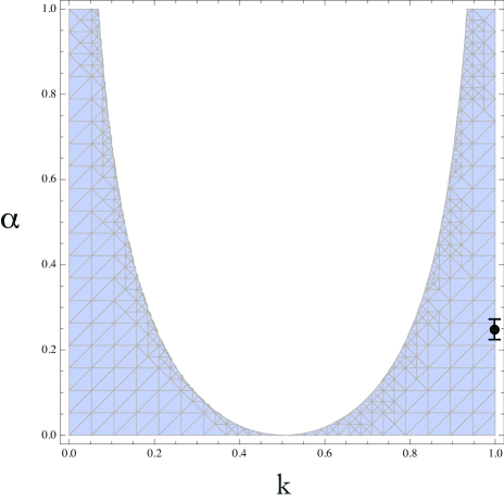
Figure 3: Plot of the transcendental relation between the $\alpha$ parameter and the modulus $k$ for the generalized Chaplygin–Jacobi gas (3.37). The shaded region corresponds to pairs that are permitted by the observational data, including the value found by del Campo using $k=1$, $\alpha=0.2587\pm 0.0009$ [32]. In this graph has been used $n_{run}=-0.003\pm 0.007$ and $n_{s}=0.968\pm 0.006$ from the Planck collaboration [45].

It is known that not only scalar curvature perturbations are generated during inflation. In addition quantum fluctuations generate transverse-traceless tensor perturbations [46], which do not couple to matter. Therefore they are only determined by the dynamics of the background metric. The two independent polarizations evolve like minimally coupled massless fields with spectrum

$$\mathcal{P}_{\mathcal{T}}=\frac{16\pi}{m_{p}^{2}}\left(\frac{H}{2\pi}\right)^{2}\bigg{|}_{aH=\widehat{\rm{k}}}.$$ (3.38)

In the same way as the scalar perturbations, it is possible to introduce the gravitational wave spectral index $n_{T}$ defined by $n_{T}\equiv\frac{d\ln\mathcal{P}_{\mathcal{T}}}{d\ln\widehat{\rm{k}}}$, that becomes $n_{T}=-2\epsilon_{H}$ . At this point, it is possible to introduce the tensor–to–scalar amplitude ratio $r\equiv\frac{\mathcal{P}_{\mathcal{T}}}{\mathcal{P}_{\mathcal{R}}}$ which becomes

$$r=4\epsilon_{H},$$ (3.39)

therefore one arrives to

$$r=6\frac{\text{dn}^{2}\left[(1+\alpha)\,\Phi\right]\,\text{sn}^{2}\left[(1+\alpha)\,\Phi\right]}{\text{cn}^{2}\left[(1+\alpha)\,\Phi\right]}.$$ (3.40)

With the help of eq. (3.32) is possible to find the relation between the tensor–to–scalar amplitude ratio and the scalar spectral index, which reads

$$r(n_{s},\alpha,k)=6\frac{(k^{\prime}+k\,\zeta)(1-\zeta)}{\zeta},$$ (3.41)

which is contracted with the measurement from Planck collaboration [45] as is showed in Figure 4.

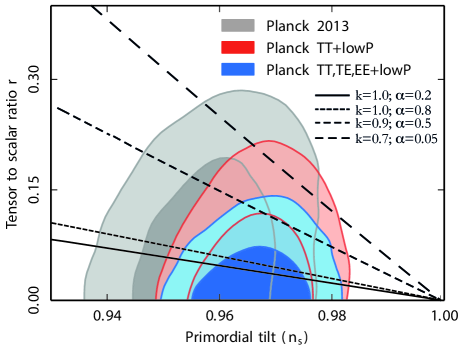
Figure 4: Plot of the parameter $r$ as a function of the scalar spectral index $n_{s}$ for the generalized Chaplygin–Jacobi gas (3.41). The marginalized joint $68\%$ and $95\%$ confidence level regions using Planck TT + low P, Planck TT, TE, EE + low P and Planck 2013 data release with $\widehat{\rm{k}}=0.05h$ Mpc^-1 are shown [45]. To perform a consistent comparison, the values of $r$ have been normalized in such a way that $r=0$ when $n_{s}=1$, and $r=16\epsilon_{H}$ is used. Note that this is four times the normalization used in this work, see equation (3.39).

4 Final remarks

This paper presents an inflationary universe model in which the inflaton field is characterized by an EoS corresponding to a generalized Chaplygin–Jacobi gas (GCJG), i.e. $p_{\phi}=-\frac{B\,k}{\rho_{\phi}^{\alpha}}-2\,k^{\prime}\,\rho_{\phi}+\frac{k^{\prime}}{B}\,\rho_{\phi}^{2+\alpha}$, where $\alpha$ is the GCG parameter, and was considered to lie in the range $0\leq\alpha\leq 1$, and the $k$ parameter is the modulus of the elliptic function which lie in the range $0\leq k\leq 1$. In this study the kinematical evolution was described using the Hubble parameter given by $H(\phi,k)=H_{0}\,\textrm{nc}^{\frac{1}{1+\alpha}}\left[(1+\alpha)\,\Phi\right]$. From here, all relevant quantities that describe inflation (scale factor, number of e-folds, deceleration parameter, etc.) were obtained in terms of Jacobian elliptic functions, allowing express them in an analytical form.

As a direct application of these analytical results, it is possible to obtain an expression relating the running scalar spectral index with the scalar spectral index (cf. equation (3.37)). Using Planck 2015 data [45], $n_{run}=-0.003\pm 0.007$ and $n_{s}=0.968\pm 0.006$, the transcendental relation in the $\alpha$–$k$ space, showed in Figure 4, was obtained. Notice del Campo [32] obtained just one value $\alpha=0.2587\pm 0.0009$ using the Planck 2013 data [34], which is in agreement with the present results. In the same way, a relation between the tensor–to–scalar ratio parameter, $r$, and $n_{s}$ is found (cf. equation (3.41)), and contrasted with the marginalized joint 68% and 95% confidence level regions using Planck TT+low P, Planck TT, TE, EE + low P and Planck 2013 release with $\widehat{\rm{k}}=0.05h$ Mpc^-1 [45]. Based on these comparisons, it can be argued that the GCJG model is very auspicious regarding the available observational tests.

Finally, since this generalization introduces a new parameter (the modulus $k$), it provides a viable opportunity to improve confrontations with the observational data. Thus, this model offers new opportunities to further investigate on the accelerated stage and interacting models.

Appendix A A brief review of Jacobian elliptic functions

As starting point, let us consider the elliptic integral [47, 48, 49, 50, 51]

$$u(y,k)\equiv u=\int_{0}^{y}\frac{dt}{\sqrt{(1-t^{2})(1-k\,t^{2})}}\\ =\int_{0}^{\varphi}\frac{d\theta}{\sqrt{1-k\sin^{2}\theta}}=F(\varphi,k),$$ (A.1)

where $F(\varphi,k)$ is the normal elliptic integral of the first kind, and $k$ is the modulus. The problem of the inversion of this integral was studied and solved by Abel and Jacobi, and leads to the inverse function defined by $y=\sin\varphi=\textrm{sn}(u,k)$ with $\varphi=\textrm{am}\,u$, and are called Jacobi elliptic sine $u$ and amplitude $u$.

The function sn $u$ is an odd elliptic function of order two. It possesses a simple pole of residue $1/k$ at every point congruent to $iK^{\prime}$ (mod $4K$, 2$iK^{\prime}$) and a simple pole of residue $-1/k$ at points congruent to $2K+iK^{\prime}$ (mod 4 $K$, $2iK^{\prime}$), where $K\equiv K(k)=F(\pi/2,k)$ is the complete elliptic integral of the first kind, $K^{\prime}=F(\pi/2,k^{\prime})$, and $k^{\prime}=1-k$ is the complementary modulus.

Two other functions can then defined by $\textrm{cn}(u,k)=\sqrt{1-y^{2}}=\cos\varphi$, which is called the Jacobi elliptic cosine $u$, and is an even function of order two; $\textrm{dn}(u,k)=\sqrt{1-k\,y^{2}}=\Delta\varphi=\sqrt{1-k\,\sin\varphi}$, called the Jacobi elliptic delta $u$ which is an even function. The set of functions $\{\textrm{sn}\,u,\,\textrm{cn}\,u,\,\textrm{dn}\,u\}$ are called Jacobian elliptic functions, and take the following special values

$$\textrm{sn}(u|0)=\sin u,\quad\textrm{sn}(u|1)=\tanh u,$$ (A.2)

$$\textrm{cn}(u|0)=\cos u,\quad\textrm{cn}(u|1)=\textrm{sech}\,u,$$ (A.3)

$$\textrm{dn}(u|0)=1,\,\qquad\,\,\textrm{dn}(u|1)=\textrm{sech}\,u.$$ (A.4)

The quotients and reciprocal of $\{\textrm{sn}\,u,\,\textrm{cn}\,u,\,\textrm{dn}\,u\}$ are designated in Glaisher’s notation by

$$\textrm{ns}\,u=\frac{1}{\textrm{sn}\,u},\quad\textrm{cs}\,u=\frac{\textrm{cn}\,u}{\textrm{sn}\,u},\quad\textrm{ds}\,u=\frac{\textrm{dn}\,u}{\textrm{sn}\,u},$$ (A.5)

$$\textrm{nc}\,u=\frac{1}{\textrm{cn}\,u},\quad\textrm{sc}\,u=\frac{\textrm{sn}\,u}{\textrm{cn}\,u},\quad\textrm{dc}\,u=\frac{\textrm{dn}\,u}{\textrm{cn}\,u},$$ (A.6)

$$\textrm{nd}\,u=\frac{1}{\textrm{dn}\,u},\quad\textrm{sd}\,u=\frac{\textrm{sn}\,u}{\textrm{dn}\,u},\quad\textrm{cd}\,u=\frac{\textrm{cn}\,u}{\textrm{dn}\,u}.$$ (A.7)

Therefore, in all, we have twelve Jacobian elliptic functions. Finally, some useful fundamental relations between Jacobian elliptic functions are

$$\textrm{sn}^{2}u+\textrm{cn}^{2}u=1,$$ (A.8)

$$\textrm{dn}^{2}u+k\,\textrm{sn}^{2}u=1,$$ (A.9)

$$\textrm{dn}^{2}u-k\,\textrm{cn}^{2}u=k^{\prime},$$ (A.10)

$$\textrm{cn}^{2}u+k^{\prime}\,\textrm{sn}^{2}u=\textrm{dn}^{2}u.$$ (A.11)

References

- [1] F. Zwicky, Die Rotverschieb ung von extragalaktischen Nebeln, Helv. Phys. Acta 6 ( 1933) 110.
- [2] H. W. Babcock, The rotation of the Andromeda nebula, Lick Observatory Bull. 498 (1939) 41.
- [3] G. Jungman, M. Kamionkowski and K. Griest, Supersymmetric dark matter, Phys. Rep. 267 (1996) 195.
- [4] L. Bergström, Non-baryonic dark matter–observational evidence and detection methods, Rep. Prog. Phys. 63 (2000) 793.
- [5] G. Bertone, D. Hooper and J. Silk, Particle dark matter: evidence, candidates and constraints, Phys. Rep. 405 (2005) 279.
- [6] L. Bergström, Dark matter candidates, New J. Phys. 11 (2009) 105006.
- [7] G. Bertone Particle Dark Matter (2009) Cambridge University Press.
- [8] P. D. Mennheim and D. Kazanas, Exact vacuum solution to conformal Weyl gravity and galactic rotation curves, Astrophys. J. 342 (1989) 635-638.
- [9] D. Kazanas and P. D. Mennheim, General structure of the gravitational equations of motion in conformal Weyl gravity, Astrophys. J. Suppl. 76 (1991) 431.
- [10] P. D. Mennheim and D. Kazanas, Solutions to the Reissner-Nordtröm, Kerr, and Kerr-Newman problems in fourth-order conformal Weyl gravity, Phys. Rev. D 44 (1991) 417.
- [11] P. D. Mennheim and D. Kazanas, Newtonian limit of conformal gravity and the lack of necessity of the second order Poisson equation, Gen. Rel. Grav. 26 (1994) 337.
- [12] A. Diaferio, L. Ostorero and V. F. Cardone, -ray bursts as cosmological probes: ΛCDM vs. conformal gravity, JCAP 10 (2011) 008.
- [13] S. Pireaux, Light deflection in Weyl gravity: Critical distances for photon paths, Class. Quant. Grav. 21 (2004) 1897-1913.
- [14] S. Pireaux, Light deflection in Weyl gravity: Constraints on the linear parameter, Class. Quant. Grav. 21 (2004) 4317-4334.
- [15] J. R. Villanueva and M. Olivares, On the null trajectories in conformal Weyl gravity, JCAP 06 (2013) 040.
- [16] S. M. Carroll, The cosmological constant, Living Rev. Relativity 4 (2001) 1.
- [17] S. Chaplygin, On gas jet, Sci. Mem. Mosc. Univ. Math. Phys. 21 (1904) 1.
- [18] A. Y. Kamenshchik, U. Moschella and V. Pasquier, An Alternative to quintessence, Phys. Lett. B 511 (2001) 265.
- [19] N. Bilic, G. B. Tupper and R. D. Viollier, Unification of dark matter and dark energy: The Inhomogeneous Chaplygin gas, Phys. Lett. B 535 (2002) 17.
- [20] J. C. Fabris, S. V. B. Goncalves and P. E. de Souza, Density perturbations in a universe dominated by the Chaplygin gas, Gen. Rel. Grav. 34 (2002) 53.
- [21] M. Makler, et al., Constraints on the generalized Chaplygin gas from supernovae observations, Phys. Lett. B 555 (2003) 1.
- [22] Z. H. Zhu, Generalized Chaplygin gas as a unified scenario of dark matter/energy: Observational constraints, Astron. Astrophys. 423 (2004) 421.
- [23] M. C. Bento, O. Bertolami, A. A. Sen, WMAP Constraints on the Generalized Chaplygin Gas Model, Phys. Lett. B 575 (2003) 172.
- [24] N. Bilic, G. B. Tupper and R. D. Viollier, Unification of dark matter and dark energy: The Inhomogeneous Chaplygin gas, Phys. Lett. B 535 (2002) 17.
- [25] M. C. Bento, O. Bertolami and A. A. Sen, Generalized Chaplygin gas, accelerated expansion and dark energy matter unification, Phys. Rev. D 66 (2002) 043507.
- [26] V. Gorini, A. Kamenshchik and U. Moschella, Can the Chaplygin gas be a plausible model for dark energy?, Phys. Rev. D 67 (2003) 063509.
- [27] M. C. Bento, O. Bertolami and A. A. Sen, Revival of the unified dark energy-dark matter model?, Phys. Rev. D 70 (2004) 083519.
- [28] S. del Campo and J. R. Villanueva, Observational Constraints On The Generalized Chaplygin Gas, Int. J. Mod. Phys. D 18 (2009) 2007.
- [29] N. Liang, L. Xu and Z. H. Zhu, Constraints on the generalized Chaplygin gas model including gamma-ray bursts via a Markov Chain Monte Carlo approach, Astron. Astrophys. 527 (2011) A11.
- [30] R. C. Freitas, S. V. B. Goncalves and H. E. S. Velten, Constraints on the generalized Chaplygin gas model from Gamma-ray bursts, Phys. Lett. B 703 (2011) 209.
- [31] H. Sandvik, et al., The end of unified dark matter?, Phys. Rev. D 69 (2004) 123524.
- [32] S. del Campo, Single-field inflation à la generalized Chaplygin gas, J. Cosmol. Astropart. Phys. 11 (2013) 004.
- [33] B. R. Dinda, S. Kumar and A. A. Sen, Inflationary generalized Chaplygin gas and dark energy in light of the Planck and BICEP2 experiments, Phys. Rev. D 90 (2014) 083515.
- [34] P. A. R. Ade et al. [Planck Collaboration], Planck 2013 results. XXII. Constraints on inflation, Astron. Astrophys. 571 (2014) A22.
- [35] J. R. Villanueva and E. Gallo, A Jacobian elliptic single–field inflation, Eur. Phys. J. C 75 (2015) 256.
- [36] B. J. Carr and J. E. Lidsey, Primordial black holes and generalized constraints on chaotic inflation, Phys. Rev. D 48 (1993) 543 .
- [37] F. E. Schunck and E. W. Mielke, A New method of generating exact inflationary solutions, Phys. Rev. D 50 (1994) 4794.
- [38] R. M. Hawkins and J. E. Lidsey, Inflation on a single brane: exact solutions, Phys. Rev. D 63 (2001) 041301.
- [39] W. H. Kinney, A Hamilton-Jacobi approach to nonslow roll inflation, Phys. Rev. D 56 (1997) 2002.
- [40] S. del Campo, Approach to exact inflation in modified Friedmann equation, J. Cosmol. Astropart. Phys. 12 (2012) 005.
- [41] H. C. Kim, Exact solutions in Einstein cosmology with a scalar field, Mod. Phys. Lett. A 28 (2013) 1350089.
- [42] A. A. Chaadaev and S. V. Chervon, New class of cosmological solutions for a self-interacting scalar field, Russ. Phys. J. 56 (2013) 725.
- [43] A. H. Guth and S. Y. Pi, Fluctuations in the New Inflationary Universe, Phys. Rev. Lett. 49 (1982) 1110.
- [44] J. M. Bardeen, P. J. Steinhardt and M. S. Turner, Spontaneous Creation of Almost Scale - Free Density Perturbations in an Inflationary Universe, Phys. Rev. D 28 (1983) 679.
- [45] P. A. R. Ade et. al., Planck 2015 results. XX. Constraints on inflation, arXiv: 1502.02114
- [46] V. F. Mukhanov, H. A. Feldman and R. H. Brandenberger, Theory of cosmological perturbations. Part 1. Classical perturbations. Part 2. Quantum theory of perturbations. Part 3. Extensions, Phys. Rept. 215 (1992) 203.
- [47] P. F. Byrd and M. D. Friedman, Handbook of Elliptic Integrals for Engineers and Scientists, 2nd ed., rev. Berlin: Springer-Verlag (1971).
- [48] H. Hancock, Lectures on the theory of elliptic functions, Dover publications Inc. New York (1958).
- [49] J. V. Armitage and W. F. Eberlein, Elliptic functions, London Mathematical Society Student Texts. (No. 67), Cambridge University Press (2006).
- [50] K. Meyer, Jacobi elliptic functions from a dynamical systems point of view, Amer. Math. Monthly 108 (2001) 729.
- [51] I. S. Gradshteyn and I. M. Ryzhik, Table of integrals, series, and products, Academic Press. (2007).