Distributed Cohesive Control for Robot Swarms:
Maintaining Good Connectivity in the Presence of Exterior Forces

Abstract

We present a number of powerful local mechanisms for maintaining a dynamic swarm of robots with limited capabilities and information, in the presence of external forces and permanent node failures. We propose a set of local continuous algorithms that together produce a generalization of a Euclidean Steiner tree. At any stage, the resulting overall shape achieves a good compromise between local thickness, global connectivity, and flexibility to further continuous motion of the terminals. The resulting swarm behavior scales well, is robust against node failures, and performs close to the best known approximation bound for a corresponding centralized static optimization problem.

I Introduction

Consider a swarm of robots that needs to remain connected. There is no central control and no knowledge of the overall environment. This environment is hostile: The swarm is being pulled apart by external forces, stretching it into a number of different directions, so it is in danger of breaking up. Individual robots are weak, with limited sensing, limited communication, and limited connectivity; even worse, each robot’s expected lifetime is limited by random, permanent failures, which may destroy connectedness and functioning of the swarm as a whole. How can we achieve coordinated dynamic swarm behavior without centralized coordination? How can we employ each robot as much as possible, without depending on it if it fails? How can we balance overall flexibility and robustness to deal with the hostile environment?

In this paper, we study swarm mechanisms that achieve these conflicting goals. Just like in the paper by Lee and McLurkin [1], we aim for algorithms that (1) maintain connectivity, (2) are fully distributed, and (3) achieve cohesiveness, i.e., a well-coordinated behavior and state for all robots. While [1] present a set of rules (based on crucial elements such as boundary recognition and boundary forces [2]) that achieve a “fat”, well-rounded swarm shape even in the presence of obstacles, this is no longer desirable in the presence of multiple outside forces that pull the swarm apart, as illustrated in Figure 1. As a consequence, we formulate a new and additional goal: (4) achieve robust and adaptive overall swarm behavior, even in the presence of external forces and node failures.

We present a combination of distributed boundary forces, density control and thickness regulation that go beyond [1] by providing results for property (4). We achieve a significant stability improvement over this and other previous approaches to flocking behavior, allowing us to face scenarios for which even the corresponding centralized, static problems are NP-hard. In a setting in which multiple dynamic terminals have to remain connected by a generalized Steiner network with limited communication range, we achieve a performance that is comparable to the best worst-case guarantee of a theoretical, centralized approximation algorithm.

Figure 1: A robust robot swarm emulating a Steiner tree between five diverging attachment points.

I-A Related Work.

One of the earliest works on flocking is Reynold’s pioneering work [3]. In recent years, a considerable number of aspects and objectives have extended this perspective. We highlight only some of the ensuing papers, showing how they differ from our perspective.

A basic component of flocking is volumetric control, as presented by Spears [4]: robots use local potential field controllers (with attractive and repulsive forces) for constructing a regular lattice with a corresponding base density [5, 6]. This does not necessarily preserve connectivity [7, 8, 4]. While the latter can be side-stepped by simply assuming that robots are always connected [9], we aim for connectivity as a requirement, which is vital in a fully distributed setting in which deterministic recovery from disconnectedness may be impossible.

Some of the ideas of Olfati-Saber [5] form the basis of our work and are discussed in more detail further down. In [5] and other work, however, robots do utilize gobal information, e.g., the position of a guide robot in a shared coordinate frame [5, 10, 11, 12] or environmental potential [13]. Instead of the potentials, Cortes et. al. [14] and Magnus et. al. [15] used Voronoi tessellation. This is based on a density function, requiring global information for covering a region. Overall, this differs from our objective of developing methods that are fully distributed, aiming for collective mechanisms for complex group behavior that go beyond relatively simple objectives [16], but also for systems that are robust against partial hardware failures [17].

The final property is “cohesiveness” of the overall swarm: all robots should maintain a unified state, such as desired distance or orientation; see [5] for a formal definition. As described in [2], detecting and maintaining a swarm boundary is of particular importance for maintaining swarm cohesiveness and connectedness. This is based on and related to work in the field of wireless sensor networks (WSNs), which has considered many geometric settings in which a large swarm of stationary nodes is faced with the task of achieving a large-scale overall goal, while the individual components can only operate locally, based on limited individual capabilities and information ([18], [19]). In addition to the work on swarm robotics described above, there is a large body of theoretical work on geometric swarm behavior; for lack of space, we only mention Chazelle [20] for flocking behavior, and Fekete et al. [18, 19] for geometric algorithms for static sensor networks, including distributed boundary detection.

Beyond the involved properties and paradigm, the overall goal for the swarm can also be described as a distributed optimization problem: Maintain a generalized Steiner tree with limited edge lengths that connects a moving set of terminals. To the best of our knowledge, only Hamann and Wörn [21] have explicitly considered the construction of Steiner trees by a robot swarm. For static terminals, they start with an exploratory network; as soon as all terminals are connected, only best paths are kept and locally optimized.

Even in a centralized and static setting with full information, we have to deal with a generalization of the well-known NP-hard problem of finding a good Steiner tree [22]. More specifically, we are faced with the relay placement problem: the input is a set of sensors and a number $r\geq 1$, the communication range of a relay. The objective is to place a minimum number of relays so that between every pair of sensors is connected by a path through sensors and/or relays. The best known theoretical performance bound for this NP-hard problem was given by Efrat et al. [23], who presented a $3.11$-approximation algorithm; they also showed a worst-case lower bound of 3 for a large class of approximation algorithms. For a fixed number of available relays, this turns into our problem of maximizing the achievable networks size, with matching approximation factor.

More specific references are given in Section III-A, where they are used as building blocks.

I-B Our contribution

We propose a set of local, self-stabilizing algorithms that maintain a dynamic and robust network between leader robots. The algorithms ensure that the swarm adopts the directions of multiple leaders, while preserving a uniform thickness along the edges of the Steiner tree. We demonstrate the usefulness of this approach by simulations with a swarm of 400 robots, five leaders and various failure rates, by showing that the resulting performance is comparable to the theoretical worst-case ratio.

II Preliminaries

We consider a finite set of robots $\mathcal{R}$. A subset $\mathcal{L}\subsetneq\mathcal{R},|\mathcal{L}|\ll|\mathcal{R}|$ of them is forced to pursue externally controlled trajectories. For simplicity, we call these leader robots; note that they have no control over their trajectories, so they have no chance to keep the swarm coherent. Instead, we want the remaining robots $\mathcal{R}\setminus\mathcal{L}$ to maintain a dynamic and robust network that keeps the swarm connected, even in the presence of random robot failures and arbitrary leader movements. Thus, the overall shape of the swarm should form a “thick” Steiner tree among the leaders with the robots $\mathcal{R}\setminus\mathcal{L}$ evenly distributed along the edges, as shown in Figure 1.

Robots have the shape of circles; two of them are connected when within a maximum distance and with an unobstructed line of sight. Robots know the relative positions and orientations of their neighbors and can communicate asynchronously. Each robot has a unique ID; leader IDs are easily made known to all others. Robot’s translations and rotations are limited in velocity and acceleration. Communication is possible by broadcasting to immediate neighbors.

The perception of all robots is local; however, due to the known position and orientation difference, each robot can transform vectors of its neighbors to its own coordinate system. We avoid multi-hop transformations to keep errors small; however, aggregate information is forwarded.

III Algorithm

The proposed approach consists of a set of local self-stabilizing mechanisms that either detect a condition or induce a force. The weighted sum of the induced forces determines the robot motion; input for the local mechanisms of the local state and environment of the robot, output is a value for current robot motion. In principle, these mechanisms are continuous. (Our simulator described later updates at 60 Hz.)

We first discuss the base behavior of the robots in Section III-A; because it has trouble with generating a non-convex swarm shape, it limits the flexibility of the swarm in the presence of external forces. This is subsequently improved by leader forces, stability improvement and thickness contraction.

III-A Base Behavior

Our base behavior consists of three components:

• The flocking algorithm of Olfati-Saber [5] considers regular distribution and movement consensus. The algorithm is a stateless equation based on potential fields and is proven to converge. It uses three rules: Attraction to neighbors, repulsion from too close neighbors, and adaption to the velocity of neighbors. We slightly modified the algorithm for better response to additional forces.

• An extended version of the boundary detection algorithm of McLurkin and Demaine [2], which determines if a robot lies on the boundary and also identifies small holes by using the average angle. In principle, the method allows the robots to distinguish exterior and interior boundaries and determine their size, but the limited precision and the convergence time limit this usage, so we only use it to detect and ignore small holes. Doing the latter is crucial for thickness and density computation, see Section III-C.

• The boundary tension of Lee and McLurkin [1], which straightens and minimizes the boundary of the swarm. This is done by simply pushing boundary robots to the middle of its two boundary neighbors.

The base swarm is similar to a water droplet and converges towards a circle after some time. The robots are well connected to the swarm and there are no attachments, as can be seen in Figure 2.

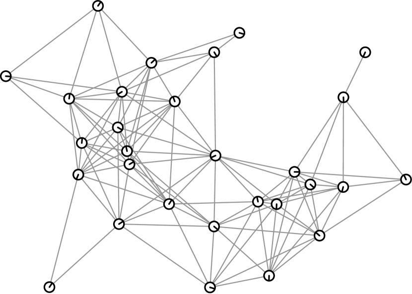
(a) Before

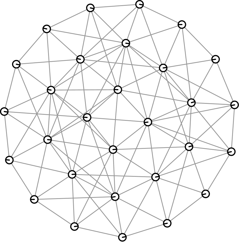
(b) After

Figure 2: The base swarm forms the swarm similar to a water drop

However, for diverging leaders the base behavior (movement consensus by flocking) without any other forces rapidly loses connectivity when the target density no longer suffices to cover the convex hull of leader robots. Figure 3 depicts a situation in which the swarm is about to lose convexity. For stronger control and more variable shapes, leader forces are introduced.

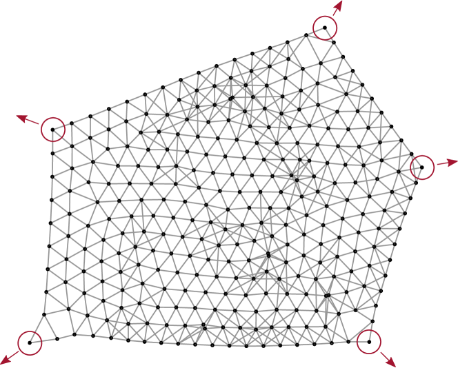
Figure 3: The base behavior without leader forces has trouble with staying connected after losing convexity.

III-B Leader Forces

A single leader constitutes the simplest form of swarm control. In this case the swarm motion is determined by the leader’s velocity. With multiple (possibly antagonistic) leaders, the swarm is not just steered, but may be stretched to the limit until connectivity is lost. Therefore, each robot needs to find an appropriate balance between the influence of different leaders. For $\ell\in\mathcal{L}$, let $c_{\ell}:\mathcal{R}\rightarrow\mathbb{R}^{2}$ be the force on a specific robot and let $d_{\ell}:\mathcal{R}\rightarrow\mathbb{N}$ be its distance to $\ell$. The leader forces on robot $r$ are combined as follows:

$$\sum_{\ell\in\mathcal{L}}c_{\ell}(r)\frac{d_{\ell}(r)^{-1}}{\sum_{\ell^{\prime}\in\mathcal{L}}d_{\ell^{\prime}}(r)^{-1}}.$$

See Figure 4 for an illustration.

Figure 4: A one-dimensional scenario with two leaders (red) moving in opposite directions.

There are two ways of following a leader: either by matching its velocity or by moving towards it. Velocity matching preserves the overall shape of the swarm, but fails with multiple leaders. However, because the velocity information needs to be passed between robots with noisy sensors, there are accumulated losses in accuracy with each hop. On the other hand, moving towards the leader causes a deformation of the swarm and can be used to control its shape when multiple leaders are used, but regions close to the leaders suffer from “compression”, which can be harmful. A combination of both methods with a smooth transition between velocity matching close to the leaders and leader pursuit when further away (see Figure 5) has a positive influence in the context of multiple leaders, both on accuracy and the overall swarm shape.

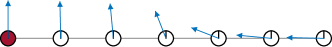
Figure 5: With increasing distance to the leader, the effect shifts from velocity matching to leader pursuit.

In order to achieve the combination of movement with the leader and towards the leader, three public variables are used for each leader. The leader distance is the minimum hop count to the leader. Let $\operatorname{pred}(r)$ be the predecessor in a minimum-hop tree to the leader, which can be the leader itself. The leader velocity is the one of $\operatorname{pred}(r)$ for a non-leader, and the robot’s own velocity for the leader. The leader direction is a normalized direction vector calculated incrementally from the direction to $\operatorname{pred}(r)$ as follows: Each robot takes the leader direction of its $\operatorname{pred}(r)$ and merges it with the normalized direction to $\operatorname{pred}(r)$. If $\operatorname{pred}(r)$ is the leader, only the normalized direction to it is used. For computing the leader force, the leader direction is scaled to the length of the leader velocity and then combined with a leader distance-sensitive weighting.

Additionally we provide leaders with too few neighbors with an attraction force, so they do not lose connection to the swarm. This attraction spreads over some distance, but decreases exponentially.

III-C Stability Improvement

Near Steiner points, connections along concave swarm boundaries may be stretched by boundary forces. When the involved edges approach the upper bound for communication, connections may be disrupted, to the point where the swarm loses connectivity. By adding a thickness-dependent compression force, we reduce neighbor distances without influencing the Steiner-tree shape of the swarm; in effect, this works similar to compression stockings. In the following, we give a heuristic for thickness computation and compression. In order to let the flocking algorithm handle this compression without destroying the regular distribution, we sketch a density distribution heuristic later in this Section. A comparison of a swarm with and without the stability improvement can be seen in Figure 6; Figure 7 shows a comparison for the same scenario with failure rate $0.008$ per second and robot.

Base	Leader	All

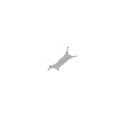
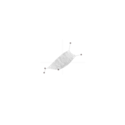
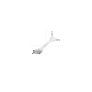
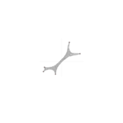
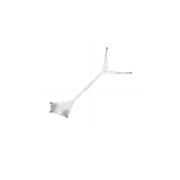
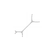
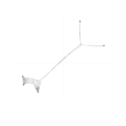
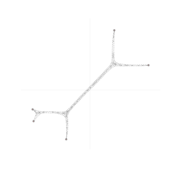
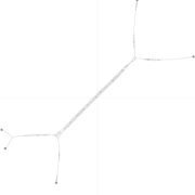
Figure 6: A comparison of strategies for the same example, for a swarm with $n=400$ and failure rate $0$. As indicated, columns correspond to strategies Base, Leader, and All. Rows show the swarms at times $T=200$, $T=2000$, $T=3000$, $T=5000$, $T=7600$, $T=12,000$, with 60 steps per simulated second. When a swarm is no longer shown, it has become disconnected right after the previous time step.

$T=4200$	$T=4400$	$T=5400$	$T=5600$

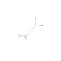
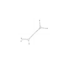
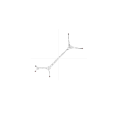
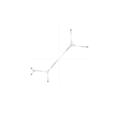
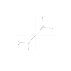
Figure 7: A comparison of strategies for the example from Figure 6, for a swarm with $n=400$, with 60 steps per simulated second and failure rate $0.008$ per second. The upper line shows the swarm with strategy Leader, the lower shows strategy All. As shown, the swarm loses connectivity at $T=4400$ (Leader), or $T=5600$ (All).

Thickness Contraction

We define the local thickness at a robot as the radius of the largest hop circle containing it. A hop circle of radius $h$ with robot $c$ as circle center is the set of all robots with a hop count $\leq h$ to $c$; only robots with distance equal to $h$ may be on the boundary. An example is highlighted in blue in Figure 8.

The relationship between geometric thickness and boundary hop distance may be distorted by long connections that skip over robots. This can be avoided by only considering edges that fulfill the edge condition of the Gabriel graph, meaning that no robot is allowed to be closer to the midpoint of an edge than the robots connected by it. In principle, the resulting communication graph equals the Gabriel Unit Disk Graph; this is the case when degenerate cases with line-of-sight obstructions are ignored. We denote the corresponding reduced neighborhood of a robot $r$ as $N^{\prime}_{r}$.

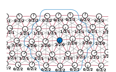
Figure 8: Thickness determination ($b(r)/t(r)/h(r)$) for a limb part. The red edges fulfill the Gabriel graph condition. A largest hop circle is marked in blue.

The following method is a simplified implementation of the thickness metric above, which performed well enough in simulation. It gets by with only three public variables; all circles with its center within a larger circle are ignored.

For this heuristic evaluation of the thickness $t(r)$ of a robot $r$, we need the hop distance $b(r)$ from the boundary and the circle center distance $h(r)$. Computing the hop distance to the boundary for each robot can easily be achieved by setting $b(r)$ to 0 for all robots on the boundary, while all others take the minimum of their neighbors plus one, as follows

$$b(r)=\begin{cases}0&\text{$r$ on boundary}\\ \min\{b(n)+1\mid n\in N^{\prime}_{r}\}&\text{else}\end{cases}$$

Small holes, that occur frequently but also vanish quickly, are excluded from the boundary, otherwise the value can become too instable. The thickness $t(r)$ is determined as the maximum $b(r)$ within some range $h(r)$, as follows.

$$t(r):=\max\{\{b(r)\}\cup\{t(n)\mid n\in N^{\prime}_{r}\wedge t(n)+\lambda\geq h(n)\}\},$$

where $\lambda\in\mathbb{N}$ is a small constant (e.g. $\lambda=2$) that tackles the problem of irregular boundaries. If $r$ is a circle center ($t(r)=b(r)$), then the circle center distance $h(r)$ is $0$. Otherwise,

$$h(r):=\min\{h(n)+1\mid n\in N^{\prime}_{r}\wedge t(n)=t(r)\}$$

An example is shown in Figure 8.

Based on this thickness $t(r)$, the described compression force grows linearly with this $t(r)$. It acts only on robots of large boundaries, so that small holes are not prevented from closing.

Density

The local density of a robot refers to the number of neighbors in relation to its observable area as shown in Figure 9. By introducing an attraction to low and repulsion from high local density neighbors, the overall swarm density is maintained at a specific homogeneous level.

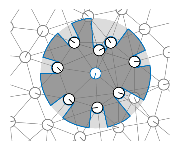
Figure 9: The observable area of a robot. The impact of hidden robots intersecting this area is ignored.

It is determined by dividing the number of neighbors by the roughly calculated observable area, cf. Figure 9. In order to avoid lumps, robots in collision range are weighted higher. Dealing with the exterior area requires particular care, because its inclusion or exclusion from the calculation skews the results. If the exterior area is included, boundary robots automatically get a lower density; if it is excluded, the density becomes too high. We account for this by considering the exterior area of a robot as the area between the two adjacent boundary neighbors. For overall balance, we assume its space to be the average space between two clockwise sequential neighbors that do not form an exterior area. A robot can lie on multiple boundaries or multiple times on the same; however, this is a sign of a sparse distribution, so we only disregard the largest one. All further exterior areas are fully included and thus lower the density.

The calculated observable area is sometimes not quite accurate, as the local knowledge is very limited. Small heterogeneities can let the values vary strongly. In order to improve the value, each robot first calculates its own value, but afterwards average this origin value with the origin values of the neighbors. This averaged value is used to determine the attraction and repulsion forces.

Let $\rho(r^{\prime})$ be the averaged local density of robot $r^{\prime}$, $\varrho$ the optimal density, and $N_{r}$ the neighbors of $r$. Then the density distribution force for a robot $r$ is given by

$$\sum_{n\in N_{r}}\overline{p}_{r}(n)*\phi(\rho(n)-\varrho),$$

where $\phi(x)=x^{3}/|x|$, and $\overline{p}_{r}:\mathcal{R}\rightarrow\mathbb{R}^{2}$ is the direction from robot $r$ to a neighbor with the length of the distance for $\rho(n)\leq\varrho$; otherwise, it is of range minus distance. We do not apply this force to robots on the boundary.

IV An Analytic Result

Before describing the performance of our approach simulation results, we discuss a related result from theoretical computer science, showing the analytic difficulty of our underlying scenario, even for a centralized, static offline scenario without node failures. In this setting, Efrat et al. [23] considered the relay placement problem, in which a given, static set of transmitters (called terminals) with limited communication range must be connected by a set of more powerful relays; the objective is to minimize the number of these relays for achieving connectivity. Clearly, this corresponds directly to the achievable scaling factor for which a connected arrangment is possible: The size of the arrangement is basically linear in the number of relays.

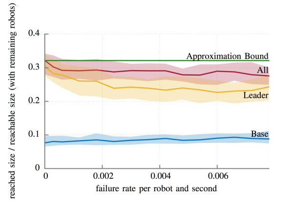
Figure 10: Relative performance of the different strategy combinations, measured by achievable Steiner tree size before disconnection occurs, compared to a hypothetical static offline optimum for the remaining live robots. Shown are median (bold) along with first and third quartiles. The failure rate is the probability of each robot to die within the next simulated second, consisting of 60 time steps. Clearly, the strategies are robust and adaptive; the full set of strategies does particularly well in adjusting to leader motion and robot failures.

As a generalization of the geometric Steiner tree problem, minimum relay placement is NP-hard. To this date, the best known approximation factor for relay placement is the following.

Theorem IV.1 (Efrat et al. [23]) There is a 3.11-approximation algorithm for minimum relay placement.

Note that this is a result for a guaranteed worst-case performance of an algorithm, so we can hope to do better in specific settings. However, we are also faced with a large number of additional difficulties that make things much more difficult: distributed setting, central control, dynamic movement of terminals the necessity to make changes dynamically without losing connectivity, as well as node failures.

V Simulation Results

We validated our approach by conducting experiments with a set of five leaders stretching out a swarm of 400 robots until it disconnects. The performance is measured against the length of the minimal Steiner tree on disconnection (calculated by the Geosteiner software [24]), divided by the theoretically maximal possible length estimated by $|\mathcal{R}^{\prime}|*\operatorname{range}$, where $\mathcal{R}^{\prime}$ are the robots that did not fail yet. This would correspond to an optimal but extremely fragile Steiner tree in which any node failure disconnects the swarm. Thus, the best possible value of 1 is completely elusive, in addition to being the result of an NP-hard offline optimization problem.

For comparison we tested three configurations: Base—only the base behavior as discussed in Section III-A; Lead—the basic behavior enriched by leader forces as discussed in Section III-B; All—the final configuration that also incorporates Density and Thickness Contraction as presented in Section III-C.

Our benchmark tests were carried out with 60 iterations per simulated second. We used parameters that correspond to those of the r-one robots of Rice University [25]: robot diameter is $10\text{\,}\mathrm{cm}$, communication range is $1.2\text{\,}\mathrm{m}$. The maximal robot velocity is $1\text{\,}\mathrm{m}\text{\,}{\mathrm{s}}^{-1}$. To account for the different source of leader motion, they were limited to at most $0.25\text{\,}\mathrm{m}\text{\,}{\mathrm{s}}^{-1}$, giving the swarm robots the opportunity to react.

For each configuration we conducted 100 random trials on a range of different failure rates; note that a failure rate of $0.006$ per second corresponds to an expected lifetime of about 167 seconds, meaning that out of 400 robots, on average about every 0.4 seconds one of them breaks down for good. Figure 10 depicts the resulting performance for all three strategies; in each case, we show the median performance, with corridors around the bold curves indicating first and third quartiles. The top part of Figure 10 gives the performance relative to a hypothetical offline optimum without robot failures, which is extremely fragile: as this solution is only a tree, any robot failure or uneven distribution will immediately disconnect it. The ratio of 0.3215 (corresponding to the performance of a 3.11-approximation algorithm for relay placement) is also indicated for better reference. The bottom part of Figure 10 gives the relative performance, compared to a hypothetical optimum that can only use the remaining live robots. It is clear to see that the strategies appear to be relatively robust against sudden disconnection due to fatal robot failure events, indicating excellent ability to adapt.

Comparing the individual strategy components, the results show that leader forces already produce decent swarm behavior, with survivability four times higher than for the base forces. Without robot losses, it reaches about 30% of the length of the hypothetical optimum, which is quite close to the theoretical approximation ratio. With robot failures, the performance gets weaker with increasing failure probability. The variant with additional stability improvement is slightly better without failures, but is clearly more robust against robot losses.

VI Conclusion

We have demonstrated how local methods for maintaining cohesiveness and connectivity of a robot swarm can achieve remarkable results, even in the presence of exterior forces and frequent, permanent robot failures.

There are numerous possible and interesting extensions. One of them is to extend our methods to heterogeneous swarms with different kinds of robots. In that setting, an even more structured, hierarchical approach may be able to combine the strengths of centralized methods (which are better suited to keep track of unbalanced situations) with the benefits of decentralized mechanisms (which are more robust against failure of key components). Clearly, this looks promising in scenarios in inhomogeneous environments, in which larger-scale, catastrophic events may cause rapid resource redistribution. Other challenges include mastering more complex tasks, such as dealing with obstacles, or performing collective transportation of objects by a swarm [26].

References

- [1] S. K. Lee and J. McLurkin, “Distributed cohesive configuration control for swarm robots with boundary information and network sensing,” in Proc. IROS. IEEE, 2014, pp. 1161–1167.
- [2] J. McLurkin and E. D. Demaine, “A distributed boundary detection algorithm for multi-robot systems,” Proc. IROS, pp. 4791–4798, 2009. [Online]. Available: http://dx.doi.org/10.1109/IROS.2009.5354296
- [3] C. W. Reynolds, “Flocking, herds, and schools: A distributed behavioral model,” Computer Graphics, vol. 21, no. 4, pp. 25–34, 1987.
- [4] W. M. Spears, D. F. Spears, J. C. Hammann, and R. Heil, “Distributed, physics-based control of swarms of vehicles,” Autonomous Robots, vol. 17, no. 2-3, pp. 137–162, 2004.
- [5] R. Olfati-Saber, “Flocking for multi-agent dynamic systems: Algorithms and theory,” IEEE Trans. Automat. Contr., vol. 51, pp. 401–420, 2006. [Online]. Available: http://dx.doi.org/10.1109/TAC.2005.864190
- [6] A. Howard, M. J. Matarić, and G. S. Sukhatme, “Mobile sensor network deployment using potential fields: A distributed, scalable solution to the area coverage problem,” in International Symposium on Distributed Autonomous Robotics Systems, 2002, pp. 299–308.
- [7] T. Balch and M. Hybinette, “Social potentials for scalable multi-robot formations,” in IEEE Int. Conf. on Rototics and Automation, 2000, pp. 73–80.
- [8] A. T. Hayes and P. Dormiani-Tabatabaei, “Self-organized flocking with agent failure: Off-line optimization and demonstration with real robots,” in IEEE Int. Conf. on Rototics and Automation, 2002, pp. 3900–3905.
- [9] H. Shi, L. Wang, T. Chu, and M. Xu, “Flocking coordination of multiple mobile autonomous agents with asymmetric interactions and switching topology,” in IEEE/RSJ International Conference on Intelligent Robots and Systems, 2005, pp. 935–940.
- [10] Y.-L. Chuang, Y. R. Huang, M. R. D’Orsogna, and A. L. Bertozzi, “Multi-vehicle flocking: Scalability of cooperative control algorithms using pairwise potentials,” in IEEE Int. Conf. on Rototics and Automation, 2007, pp. 2292–2299.
- [11] H. M. La and W. Sheng, “Flocking control of a mobile sensor network to track and observe a moving target,” in IEEE/RSJ Int. Conf. on Intelligent Robots and Systems, 2009, pp. 3129–3134.
- [12] ——, “Adaptive flocking control for dynamic target tracking in mobile sensor networks,” in IEEE/RSJ Int. Conf. on Intelligent Robots and Systems, 2009, pp. 4843–4848.
- [13] V. Gazi, “Swarm aggregations using artificial potentials and sliding-mode control,” IEEE Trans. on Robotics, vol. 21, no. 6, pp. 1208–1214, 2005.
- [14] J. Cortes, S. Martinez, T. Karatas, and F. Bullo, “Coverage control for mobile sensing networks,” IEEE Trans. on Robotics and Automation, vol. 20, no. 2, pp. 243–255, 2004.
- [15] M. Lindhé, P. Ögren, and K. H. Johansson, “Flocking with obstacle avoidance: A new distributed coordination algorithm a new distributed coordination algorithm based on voronoi partitions,” in International Conference on Robotics and Automation, 2005, pp. 1785–1790.
- [16] E. Bonabeau and C. Meyer, “Swarm intelligence: A whole new way to think about business,” Harvard Business Review, pp. 106–114, 2001.
- [17] A. Kamimura, S. Murata, E. Yoshida, H. Kurokawa, K. Tomita, and S. Kokaji, “Self-reconfigurable modular robot–experiments on reconfiguration and locomotion,” in Proceedings of the 2001 IEEE/RSJ International Conf. on Intelligent Robots and Systems, IROS 2001, vol. 1, 2001, pp. 606–612.
- [18] S. P. Fekete and A. Kröller, “Geometry-based reasoning for a large sensor network,” in Proc. SoCG, 2006, pp. 475–476. [Online]. Available: http://doi.acm.org/10.1145/1137856.1137926
- [19] A. Kröller, S. P. Fekete, D. Pfisterer, and S. Fischer, “Deterministic boundary recognition and topology extraction for large sensor networks,” in Proc. SODA, 2006, pp. 1000–1009. [Online]. Available: http://dl.acm.org/citation.cfm?id=1109557.1109668
- [20] B. Chazelle, “The convergence of bird flocking,” J. ACM, vol. 61, no. 4, p. 21, 2014.
- [21] H. Hamann and H. Wörn, “Aggregating robots compute: An adaptive heuristic for the euclidean steiner tree problem,” in From Animals to Animats 10. Springer, 2008, pp. 447–456. [Online]. Available: http://dx.doi.org/10.1007/978-3-540-69134-1˙44
- [22] M. R. Garey, R. L. Graham, and D. S. Johnson, “The complexity of computing Steiner minimal trees,” SIAM J. Appl. Math., vol. 32, no. 4, pp. 835–859, 1977.
- [23] A. Efrat, S. P. Fekete, P. Gaddehosur, J. Mitchel, V. Polishchuk, and J. Suomela, “Improved approximation algorithms for relay placement,” in Algorithms-ESA, ser. Springer LNCS, vol. 5193, 2008, pp. 356–367.
- [24] D. Warme, P. Winter, and M. Zachariasen, “Geosteiner 3.1,” Department of Computer Science, University of Copenhagen (DIKU), 2001.
- [25] J. McLurkin, A. J. Lynch, S. Rixner, T. W. Barr, A. Chou, K. Foster, and S. Bilstein, “A low-cost multi-robot system for research, teaching, and outreach,” in Distributed Autonomous Robotic Systems - The 10th International Symposium, DARS 2010, Lausanne, Switzerland, November 1-3, 2010, 2010, pp. 597–609.
- [26] M. Rubenstein, A. Cabrera, J. Werfel, G. Habibi, J. McLurkin, and R. Nagpal, “Collective transport of complex objects by simple robots: theory and experiments,” in International conference on Autonomous Agents and Multi-Agent Systems, AAMAS ’13, Saint Paul, MN, USA, May 6-10, 2013, 2013, pp. 47–54.